A Comparison of Machine Learning Techniques for the Quality Classification of Molded Products

Abstract

The developments in the internet of things (IoT), artificial intelligence (AI), and cyber-physical systems (CPS) are paving the way to the implementation of smart factories in what is commonly recognized as the fourth industrial revolution. In the manufacturing sector, these technological advancements are making Industry 4.0 a reality, with data-driven methodologies based on machine learning (ML) that are capable of extracting knowledge from the data collected by sensors placed on production machines. This is particularly relevant in plastic injection molding, with the objective of monitoring the quality of molded products from the parameters of the production process. In this regard, the main contribution of this paper is the systematic comparison of ML techniques to predict the quality classes of plastic molded products, using real data collected during the production process. Specifically, we compare six different classifiers on the data coming from the production of plastic road lenses. To run the comparison, we collected a dataset composed of the process parameters of 1451 road lenses. On such samples, we tested a multi-class classification, providing a statistical analysis of the results as well as of the importance of the input features. Among the tested classifiers, the ensembles of decision trees, i.e., random forest and gradient-boosted trees (GBT), achieved 95% accuracy in predicting the quality classes of molded products, showing the viability of the use of ML-based techniques for this purpose. The collected dataset and the source code of the experiments are available in a public, open-access repository, making the presented research fully reproducible.

1. Introduction

The advancements in the internet of things (IoT), artificial intelligence (AI), and Cyber-Physical Systems (CPS) are leading the manufacturing sector towards a fourth industrial revolution [1]. Part of this technological leap, named “Industry 4.0”, involves the development of smart factories, i.e., production systems capable of self-organizing, predicting, and correcting their own faults, and that can adapt to variable human needs [2]. The increasing availability of pervasive sensors makes AI and, specifically, machine learning (ML) pivotal for the Industry 4.0 transition, enabling the operation of industries in a flexible, efficient, and green way [3]. In fact, data-driven methodologies based on ML and deep learning (DL) are emerging in several Industry 4.0 applications, such as anomaly detection [4], predictive maintenance [5,6], inventory management [7], sensory and productivity measurements [8,9], aided design [10], quality control [11], security [12], smart working [13], digital twin development [14], healthcare [15,16], and many others [17].

Plastic injection molding is a manufacturing process widely used in the industry [18], as it allows for the production of plastic objects characterized by complex geometries with high precision and productivity [19]. Specifically, the process includes four phases, i.e., plasticization, injection, packing, and cooling [20], during which the polymer is melted, injected and compressed in the mold, and, eventually, cooled. Given that the quality of a molded product depends on the process parameters, as optimal values reduce the cycle time and increase the quality of the final product [21], extensive research has been devoted to predict the quality of products from the value of the production process parameters. Whilst early research works are dated back to the first decade of 2000, using techniques such as support vector machine (SVM) [22] and neural networks [20,23], the advent of Industry 4.0 and its focus on extracting knowledge from machine sensors have boosted interest about the application of ML methods for the prediction of product quality from the parameters of the production process [24,25,26,27].

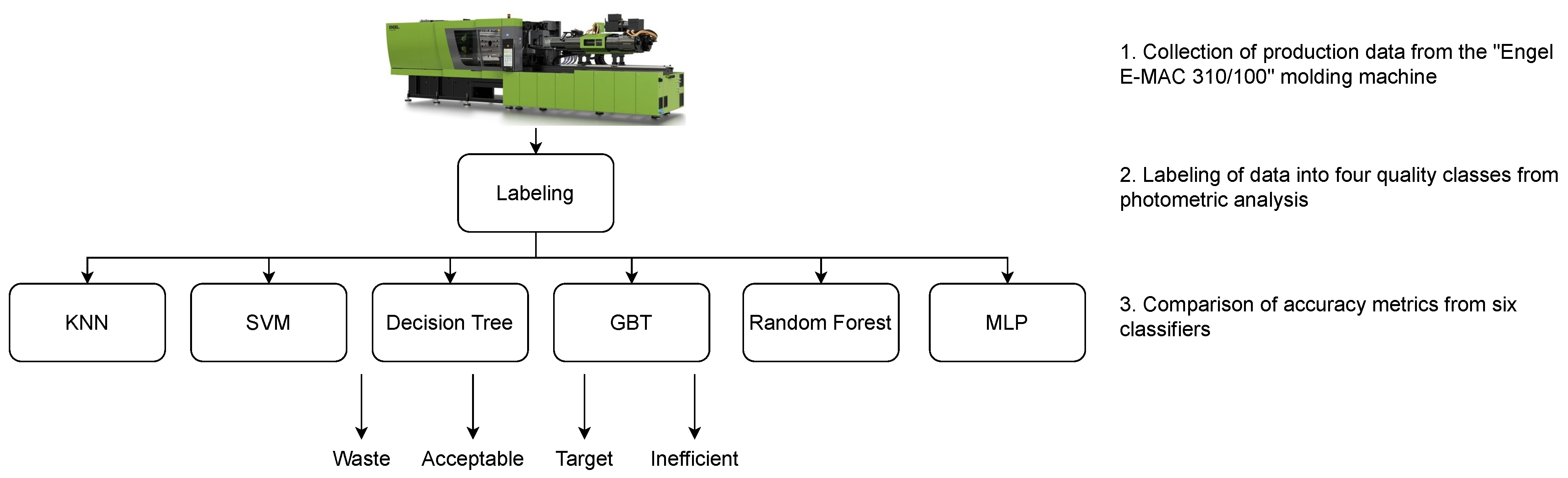
In this regard, this paper investigates the effectiveness of ML techniques to predict the quality of molded plastic products from the production process parameters, using real data from in-line industrial measurements. Specifically, the data comes from the production of plastic road lenses of “iGuzzini Illuminazione”, a company located in Recanati, Italy, which specializes in providing plastic components for lighting devices. In fact, road lenses are regulated by the standard “UNI EN 13201-2:2016”, which sets threshold values for the lighting uniformity ($U_0$). Currently, controlling the quality of the lenses, i.e., their lighting uniformity, requires a lens-by-lens photometric analysis conducted by specialized personnel in lab settings, demanding significant resources. Therefore, our aim is to understand if this control can be automated or, at least, integrated by using ML methods to estimate the level of the lighting uniformity of a lens from its process parameters collected by the sensors of the injection molding machine during the production.

The research conducted on the “iGuzzini Illuminazione” case study and that is described in this paper adds the following contributions to the state of the art of quality prediction in injection molding:

• A real application of Industry 4.0 is demonstrated, proposing the use of ML to automate the quality control of molded plastic products;
• A comparison of six ML techniques for quality prediction is provided. The tested techniques are K-nearest neighbor (KNN), decision tree, random forest, gradient-boosted trees (GBT), support vector machine (SVM), and multi-layer perceptron (MLP). The source code of the comparison is publicly available in a GitHub repository (https://github.com/airtlab/machine-learning-for-quality-prediction-in-plastic-injection-molding, accessed on the 15 May 2022);
• A new dataset is presented. It includes the real data about the production of road lenses by injection molding and is publicly available in the source code repository. As such, the dataset can be used to benchmark other techniques.

Despite the number of research works about quality prediction in plastic injection molding available, most of the papers compare few techniques (one or two) on often-unbalanced datasets with few samples, as explained in the literature review included in Section 2. Moreover, most of the papers distinguish between good products and faulty products. Instead, we compare six different techniques on a dataset collecting the production process parameters of 1451 samples, i.e., road lenses. Moreover, we classify the road lenses in four different quality classes, instead of dealing with a binary problem. Furthermore, to the best of our knowledge, this is the first work in quality prediction for plastic injection molding to publicly release the source code of the comparison of ML techniques and the data used for the tests, providing fully reproducible results.

The rest of the paper is organized as follows. Section 2 lists other relevant research works on quality prediction for plastic injection molding, comparing our methodology to the related literature. Section 3 describes the dataset built for the experiments and the compared ML techniques, providing the necessary background. Section 4 presents an experimental evaluation of the quality prediction applied to the production of the road lenses, discussing the results. Finally, Section 5 draws the conclusions of this research.

2. Literature Review

Early research works for quality prediction in plastic injection molding are dated back to the early 2000s. For example, Sadeghi [23] proposed a neural network and a multi-layer perceptron (MLP) using four features (melt flow rate, injection pressure, mold temperature, and melt temperature) to estimate actual injection pressure, filling time, and part soundness, with a hidden layer composed of two neurons. The author tested the proposed methodology on simulated data. Similarly, Chen et al. [20] used a neural network-based approach to estimate the weight of the samples. They combined self-organizing maps (SOM), using three features as inputs (injection stroke curve, injection velocity curve, and pressure curve), and an MLP, using six features as inputs (injection time, VP switch position, packing pressure, injection velocity, packing time, and injection stroke), on 160 real samples (120 for training, 40 for testing), achieving a root mean squared error of 0.0017. Ribeiro [22] proposed the use of support vector machine (SVM) classifiers to predict faults in automotive parts produced with injection molding. They used six features as the input (cycle time, metering time, injection time, barrel temperature before nozzle, cushion, and injection velocity) and compared their methodology with a neural network to predict six types of faults, obtaining an accuracy between 87% and 100% (depending on the type of fault to be classified). Liu et al. [28] proposed an ensemble of neural networks to predict the shrinkage of thin shell parts as a measure of their quality. They used mold temperature, holding pressure, and holding time as inputs for the neural networks, taking 70 samples for training, 15 samples for validation, and 15 samples for testing, achieving a top root mean squared error of 0.008.

Differently from the listed early research works, we compare more techniques (six), on more real data (our dataset is composed of the process parameters of 1451 samples), using more features (thirteen), and applying a cross-validation scheme to generalize the results.

After Industry 4.0 became an established paradigm exploiting IoT, AI, and CPS to increase efficiency and productivity in manufacturing, several research works devoted their efforts to predicting the quality of molded plastic products. For example, Nagorny et al. [24] proposed the use of convolutional neural networks (CNNs) to process thermographic images of products and long short-term memory (LSTM) neural networks to process raw parameters and to run the regression of a single-quality attribute. They tested their approach on a dataset composed of 177 samples for training and 27 samples for testing. They compared their methodology with classical regression algorithms, achieving the best results with the LSTM. Instead of calculating the regression of a single variable, we use a classification approach to predict the quality classes of road lenses, and we train and test on a bigger dataset. Ogorodnyk et al. [25] compared an MLP and a decision tree classifier (J48) using 18 features as inputs. They used a 10-fold cross-validation scheme on a dataset composed of 101 defective samples and 59 good samples. They achieved the best results with the decision tree, obtaining 95.6% accuracy. Differently from their work, our dataset is almost balanced and includes more samples. Furthermore, we classify the samples into four quality classes, instead of performing a binary classification. Obregon et al. [29] compared different ensembles of decision trees on an imbalanced binary dataset, with the objective of inferring explainable rules for quality control. In their first experiment, they used a dataset composed of 81 normal products and 37 defective products, whereas, in the second, they had 287 normal products and 613 defective products, achieving a top accuracy of 94.98% in the first experiment, and 99.73% in the second. Ke and Huang [26] proposed an MLP with a hidden layer to predict classes of three width measures of the molded products. As inputs, they took four parameters measured in ten different points of the injection molding process. They trained their model on 356 samples and tested on 89 samples, obtaining an accuracy around 90% (with a class scoring of 93% as the best result). Jung et al. [27] compared an autoencoder against several classical ML techniques on a very imbalanced dataset composed of 5617 samples, using 70% of the data as the training set and 30% of the data as the test set. Specifically, the test set included 1605 good samples and only 125 defective samples. They achieved a 99% accuracy with the autoencoder on their binary problem. Differently from these research works, we tested our models on a balanced dataset and on a multi-class problem.

Deep neural networks (DNNs) and DL-based techniques demonstrate their effectiveness in pattern recognition for many different applications, such as image and video processing, object detection, speech recognition, and others [30]. DNNs and DL-based techniques have been recognized as useful even for industrial quality prediction, providing better results than shallow networks in different applications [31]. For example, Liu et al. [32] proposed a novel stacked multi-manifold autoencoder for feature extraction, and successfully applied it to quality prediction in the hydrocracking process. Instead, in our research, we try to classify the quality of molded products from 1451 feature vectors with the parameters of the plastic injection molding process. As such, the amount of available data, its tabular nature, and the need of using only real data, without simulated or synthetic values, led us to the choice of applying classical ML techniques on hand-crafted features. However, DL-based techniques are emerging, even in plastic injection molding, and try to apply transfer learning to deal with the scarcity of training data, such as in [33,34].

Moreover, differently from all the works listed in this section, we publicly released the source code and the data of the tests, providing fully reproducible experiments.

3. Materials and Methods

Figure 1 outlines the methodology implemented in the research described in this paper. We built a dataset with the process parameters corresponding to the production of 1451 road lenses, collected during different production days. Then, we defined four quality classes to label the lenses in our dataset by measuring their general uniformity ($U_0$) with the manual photometric analysis in lab settings. To understand the viability of the quality prediction, we compared six different classifiers by collecting accuracy metrics. To select the best hyperparameters for each classifier, we applied a grid search strategy.

In the following, we provide a detailed description of the dataset that we used for the comparison (Section 3.1), as well as a description of the hyperparameters tested for each classifier (Section 3.2).

3.1. Plastic Injection Molding Data

The experimental evaluation consists of tests executed on a dataset composed of 1451 feature vectors corresponding to 1451 road lenses produced by iGuzzini Illuminazione. The data was collected from the sensors of the “Engel E-MAC 310/100” injection machine (https://www.engelglobal.com/en/us/index.html, accessed on the 15 May 2022), with the “TIG” Manufacturing Execution System (MES) (https://www.tig-mes.com/en/, accessed on the 15 May 2022), during five different production days, namely, the 18th, 19th, and 20th of September 2019, the 7th of February 2020, and the 20th of May 2020. Each feature vector includes 13 injection molding process parameters (

Table 1. The process parameters included in the feature vector of each sample in the dataset.

Feature	Unit	Description
Melt temperature	°C	Temperature of the polymer before the injection in the mold
Mold temperature	°C	Temperature of the mold
Filling time	s	Time to fill the mold
Plasticizing time	s	Time to plasticize the product
Cycle time	s	Time to complete the entire process for a product
Closing force	N	Closing force of the mold
Clamping force peak value	N	Peak value of the closing force of the mold
Torque peak value current cycle	N·m	Peak value of the torque on the injection screw
Torque mean value current cycle	N·m	Mean value of the torque on the injection screw
Specific back pressure peak value	Bar	Peak value of the resistance of the injection screw
Specific injection pressure peak value	Bar	Peak value of the injection pressure
Screw position at the end of hold pressure	cm	Position of the injection screw at the end of the holding cycle
Shot volume	cm3	Injection volume

), namely, the melt temperature (°C), the mold temperature (°C), the filling time (s), the plasticizing time (s), the cycle time (s), the closing force (N), the clamping force peak value (N), the torque peak value (N·m), the torque mean value (N·m), the back pressure peak value (bar), the injection pressure peak value (bar), the screw position at the end of the hold pressure (cm), and the shot volume (cm³).

Given that the standard “UNI EN 13201-2:2016” imposes a general uniformity $U_0$ greater than 0.4 for M1 lenses in motorized roads, we defined the following four quality classes for the samples of the dataset:

• Waste, with $U_0<0.4$. All the samples that exhibit a general uniformity less than 0.4 in the photometric analysis should be discarded, as they are not compliant to the standard. The label for this class is 1;
• Acceptable, with $0.4\le U_0<0.45$. All the samples with a uniformity greater than or equal to 0.4 and less than 0.45 are considered acceptable by iGuzzini Illuminazione, as they comply with the standard. However, the target for the iGuzzini production is a higher quality. The label for this class is 2;
• Target, with $0.45\le U_0\le 0.5$. All the samples with a uniformity greater than or equal to 0.45 and less than or equal to 0.5 are considered optimal by the company. The label for this class is 3;
• Inefficient, with $U_0>0.5$. Even if the general uniformity is far greater than the standard threshold, producing lenses with a uniformity greater than 0.5 would result in the molding machine using more resources; therefore, this quality should be avoided, given that it is not required. The label for this class is 4.

Table 2. The number of samples for each class in the proposed dataset.

	Waste	Acceptable	Target	Inefficient
Label	1	2	3	4
# Samples	370	406	310	360

describes the division of the 1451 samples included in the dataset into the four classes: 370 lenses are labeled as Waste, 406 lenses as Acceptable, 310 as Target, and 360 as Inefficient.

We evaluated the relevance of each feature on the class labels by scoring each feature according to the Relief algorithm [35] and the analysis of variance (ANOVA) method [36]. To this end, Figure 2 shows the feature scores computed with the Relief algorithm, normalized between 0 and 1. The feature with the highest score is the cycle time, i.e., the time to complete the molding process for a single sample. The filling time is the second-best feature, whereas the melt temperature and the specific back pressure have the lowest values.

The ANOVA statistic confirms that the most relevant feature is the cycle time, as per Figure 3. However, the importance of the other features is relatively low compared to the cycle time. In fact, normalizing the computed ANOVA F-values between 0 and 1, the cycle time has an importance of 1, whereas the second-best feature is the specific injection pressure, with a weight equal to 0.0295, and the third best feature is the mold temperature, with a weight of 0.0289.

3.2. Tested ML Techniques

To understand the feasibility of predicting the quality of the samples, i.e., the uniformity of the road lenses in the dataset, we tested six different classifiers, implementing the most used in the related literature, as described in Section 2. Specifically, we tested K-nearest neighbor (KNN), decision tree, random forest, gradient-boosted trees (GBT), support vector machine (SVM), and multi-layer perceptron (MLP) methods. For all the models, we looked for the hyperparameters which gave the best classification accuracy using an exhaustive grid search strategy. All the classifiers were implemented in RapidMiner Studio 9.10 (https://rapidminer.com/, accessed on the 15 May 2022), using a stratified 5-fold cross-validation scheme for the evaluation. In the following, we provide the details of each tested classifier.

3.2.1. KNN

K-nearest neighbor (KNN) is one of the most known and simple classification techniques. It classifies the feature vector of an unknown sample by using the most common label among the k feature vectors in the training set, which are the nearest (i.e., the most similar) to the unknown sample. Therefore, the hyperparameters of a KNN classifier are:

• The K value, to establish how many neighbors should be considered to predict the class of an unknown sample. We tested all possible K values between 1 and 100;
• The distance measure to evaluate the similarity between feature vectors. Given that the features are numerical, we tested the Euclidean distance, cosine similarity, and Manhattan distance.

Table 3. The top six combinations of hyperparameters for the KNN. The best accuracy was achieved with $K=4$ by using the Manhattan distance to measure the similarity between the feature vectors.

K	Distance	Accuracy
4	Manhattan	92.21%
6	Manhattan	91.73%
3	Manhattan	91.73%
5	Manhattan	91.73%
8	Manhattan	91.46%
7	Manhattan	91.32%

shows the top six KNNs in terms of accuracy. Among the 300 possible variants of the KNN resulting from the combination of these hyperparameters, we obtained the best accuracy (92.21%) for $K=4$ with the Manhattan distance. In general, the Manhattan distance showed better accuracy than the Euclidean distance and the cosine similarity, even for different K values.

3.2.2. Decision Tree

A decision tree is a tree-like structure where each node is a test on one of the attributes of a feature vector and each leaf is a class label. The objective is to infer classification rules from the features of the training set. As such, a path from the root of the decision tree to a leaf is a set of classification rules used to assign a label to a sample. We evaluated 88 different decision trees, resulting from the combination of the following hyperparameters:

• The maximum depth of the tree, testing 10 different steps (with a linear increase) inside the range [−1, 300], i.e., all the possible values in the set {−1, 29, 59, 89, 119, 150, 180, 210, 240, 270, 300}, where −1 represents “no maximum depth”;
• The splitting criterion to select the features that best separate the input data, testing information gain, gain ratio, gini index, and accuracy;
• The use of pre-pruning, using the following three criteria, in addition to the maximum depth:

  −

  Gain when splitting a node lower than 0.01 (i.e., minimal gain = 0.01);

  −

  Number of samples in a leaf lower than 2 (i.e., minimal leaf size = 2);

  −

  Number of samples per split lower than 4 (i.e., minimal size for split = 4).

Moreover, we applied an error post-pruning using a confidence value equal to 0.1.

Table 4. The top six combinations of hyperparameters for the decision tree. The best performance was achieved by using the accuracy as the splitting criterion for the nodes of the tree, without applying any pre-pruning strategy. The maximum depth had no effect, given that the tree stopped before reaching a depth of 29, which was the minimum tested.

Pre-Pruning	Split Criterion	Accuracy
false	accuracy	91.52%
true	accuracy	91.45%
true	Gini index	90.08%
true	information gain	89.59%
false	Gini index	89.46%
false	gain ratio	89.46%

lists the top six decision trees in terms of accuracy. We obtained the best result (91.52%) with the accuracy splitting criterion, without using the pre-pruning. Instead, the maximum depth had no impact on the final accuracy of the decision tree classifier in our case study, as the tree never reached the lowest maximum depth (29). The best result using pre-pruning was also achieved with the accuracy splitting criterion (91.45% accuracy), whereas the best result achieved by another splitting criterion was 90.08% accuracy, obtained by the Gini index (with pre-pruning).

3.2.3. Random Forest

A random forest is a classifier which consists of an ensemble of decision trees independently trained by bagging the samples in the training set and the features for each tree. A new input is classified according to a voting mechanism applied to the results of all the trees created in the random forest. Specifically, we used extremely randomized trees (ExtraTrees) [37], which means that:

• No pruning strategy was applied;
• The number of features to evaluate for the split in each tree was equal to $int\left(log\right(m)+1)$, where m is the number of features;
• The features to be used for the split in a tree were randomly selected.

We tested 484 different variants of the random forest with our dataset, looking for the best accuracy by tuning the following hyperparameters:

• The maximum number of decision trees in the random forest, testing 10 different steps (with a linear increase) inside the range [−1, 300], i.e., all the values in the set {1, 31, 61, 91, 121, 151, 180, 210, 240, 270, 300};
• The maximum depth of the trees, testing 10 different steps (with a linear increase) inside the range [−1, 200], i.e., all the possible values in the set {−1, 19, 39, 59, 79, 100, 120, 140, 160, 180, 200}, where −1 represents “no maximum depth”;
• The splitting criterion to select the features that best separate the input data, testing information gain, gain ratio, Gini index, and accuracy.

The minimal gain for the trees was 0.01, the minimal leaf size was 2, and the minimal size for splitting was 4. The confidence voting strategy was applied, predicting the class of a new sample using the label with the highest accumulated confidence (summing up all the trees).

Table 5. The top six combinations of hyperparameters for the random forest. The best performance was achieved by using the gain ratio as the splitting criterion for the nodes of the tree, using 151 trees, and with 79 as the maximum depth. No pruning strategies were applied, as we used the extremely randomized trees method. A maximum depth of −1 represents that no maximum depth was used for the trees.

# Trees	Max Depth	Split Criterion	Accuracy
151	79	gain ratio	95.04%
300	−1	gain ratio	94.97%
210	79	gain ratio	94.90%
61	−1	gain ratio	94.90%
270	−1	gain ratio	94.90%
121	39	gain ratio	94.90%

includes the top six combinations of hyperparameters for the random forest. We obtained the best accuracy (95.04%) using 151 trees, with the maximum depth set to 79, and using the gain ratio as the criterion for the splits. The second-best splitting criterion (94.68% accuracy) was the information gain, with 151 trees and with 140 as the maximum depth.

3.2.4. GBT

Like the random forest, the gradient-boosted trees (GBT) method is an ensemble of decision trees. However, different from random forests, the trees are not trained independently. Instead, trees are trained sequentially, to gradually produce better predictions, with each tree attempting to correct the squared error of its predecessor. The class of a sample is then predicted as a weighted majority of the trees, where the weights are proportional to the accuracy of each tree. We compared 121 variants of GBT, resulting from the combination of the following hyperparameters:

• The maximum number of decision trees in the random forest, testing 10 different steps (with a linear increase) inside the range [1, 300], i.e., all the values in the set {1, 31, 61, 91, 121, 151, 180, 210, 240, 270, 300};
• The maximum depth of the trees, testing 10 different steps (with a linear increase) inside the range [1, 200], i.e., all the possible values in the set {1, 21, 41, 61, 81, 101, 120, 140, 160, 180, 200}.

All the samples and features were used for each tree, with a shrinkage (learning rate) equal to 0.01.

Table 6. The top six combinations of hyperparameters for the GBT. The best performance was achieved by using 300 trees with a maximum depth of 41 (and all the values above 41). The second-best accuracy is slightly lower, given by 270 trees with a maximum depth of 41 (and above).

# Trees	Max Depth	Accuracy
300	41 (and above)	94.21%
270	41 (and above)	94.14%
300	21	94.07%
240	21 (and above)	94.00%
210	41 (and above)	93.87%
210	21	93.80%

lists the top six combinations of hyperparameters for the GBT. The best accuracy (94.21%) was obtained by the GBT composed of 300 trees, with a maximum depth of 41.

3.2.5. SVM

A support vector machine (SVM) classifier builds a set of hyperplanes that separate the training data into two classes, constructing a classification boundary in the feature space of the samples. To be adapted to multi-class problems, one-versus-one and one-versus-rest approaches can be followed. The RapidMiner implementation, based on LibSVM (https://www.csie.ntu.edu.tw/~cjlin/libsvm/, accessed on the 15 May 2022), uses the one-versus-one approach, building a binary SVM for all the possible couples of classes and using a majority voting strategy to label a new sample from the binary SVMs’ outputs. We compared 36 variants of SVMs on our dataset, given by the combination of the following hyperparameters:

• The C hyperparameter, regulating the margin from the decision boundary, testing 3 different steps (with a logarithmic increase) inside the range [0.1, 100], i.e., all the values in the set {0.1, 1, 10, 100};
• The kernel function, testing a linear kernel, a sigmoid kernel, a polynomial kernel, and a radial basis function (RBF) kernel. With the RBF kernel, we compared different values for the $Gamma$ parameter, testing 5 steps (with a logarithmic increase) inside the range [0.0001, 10], i.e., all the values in the set {0.0001, 0.001, 0.01, 0.1, 1, 10}.

Table 7. The top six combinations of hyperparameters for the SVM classifier. The best performance was achieved using the RBF kernel, with $C=100$ and $Gamma=0.001$. In terms of accuracy, the top five configurations used the RBF kernel. Among the other kernels, the polynomial worked better than the linear and the sigmoid, achieving 89.39% accuracy with $C=0.1$.

C	Gamma	Kernel	Accuracy
100.0	0.0010	rbf	91.73%
10.0	0.0100	rbf	91.32%
10.0	0.0010	rbf	90.90%
1.0	0.0100	rbf	90.63%
100.0	0.0001	rbf	89.94%
0.1	-	polynomial	89.39%

shows the top six combinations of hyperparametrs for the SVM classifier. We obtained the best accuracy result (91.73%) with the SVM based on the RBF kernel, with $C=100$ and $Gamma=0.01$. The top five combinations are based on the RBF kernel, whereas the best among the other kernels is the polynomial, scoring 89.39% accuracy with $C=0.1$.

3.2.6. MLP

A multi-layer perceptron (MLP) is a feed-forward neural network in which each layer is fully connected to the next one. In addition to the input layer, which maps the feature vector of the samples, and an output layer, which maps the classes to be predicted, it includes one or more hidden layers. For the architecture of the MLP tested in this paper, we followed the results from Ke and Huang [26], using a hidden layer composed of six neurons, between the input layer (13 neurons, given that the features of each sample are 13) and the output layer (4 neurons, consistent with the number of classes in our dataset). We compared 48 variants of the MLP, combining the following hyperpameters:

• The learning rate, testing 3 different steps with logarithmic increase in the range $[0.0001, 0.1]$, i.e., all the values in the set $\{0.0001,$$0.001,$$0.01,$$0.1\}$;
• The momentum for the gradient descent, testing 3 steps with linear increase in the range $[0.6, 0.9]$, i.e., all the values in the set $\{0.6,$$0.7,$$0.8,$$0.9\}$;
• The number of epochs for the training process, testing 3 steps with linear increase in the range $[100, 500]$, i.e., all the values in the set $\{100,$$300,$$500\}$.

In addition, the minimum error to stop optimization was 0.0001, whilst no decay for the learning rate was applied. The activation function for each neuron is the sigmoid, and the inputs were normalized between −1 and 1.

Table 8. The top six combinations of hyperparameters for the MLP. The network trained for 500 epochs with a learning rate of 0.1 and a momentum of 0.6 achieved the best accuracy.

Learning Rate	Momentum	Epochs	Accuracy
0.1000	0.6	500	92.08%
0.1000	0.7	500	91.94%
0.0100	0.9	500	91.59%
0.1000	0.7	300	91.39%
0.1000	0.8	100	91.11%
0.1000	0.7	100	90.63%

lists the top six combinations of the hyperparameters for the MLP. The network with a 0.1 learning rate, 0.6 momentum, and 500 epochs achieved the best accuracy (92.08%).

4. Experimental Evaluation

We compared the six classifiers on the dataset composed of the 1451 feature vectors with the process parameters collected during the production of road lenses. In this section, we report the details about the results achieved by the best configuration of each classifier, as explained in Section 3.2. In fact, we want to understand if the ML-based classifiers can be used for the quality prediction in the iGuzzini Illuminazione case study. In addition to the creation of a baseline of metrics on the collected dataset, a comparison of classifiers might be relevant to other case studies about quality prediction from the production process parameters in plastic injection molding.

Therefore, in the following subsections, we describe the experimental setup as well as the evaluation metrics (Section 4.1) used to compare the classifiers. Moreover, we present and analyze the results of the evaluation (Section 4.2). Finally, we discuss the limitations of our experimental evaluation (Section 4.3).

4.1. Experimental Setup and Evaluation Metrics

To assess the viability of the use of ML techniques to predict the quality of road lenses from the parameters of the production process, we implemented the proposed classifiers in RapidMiner Studio 9.10. The tests ran on a Windows 10 notebook equipped with an i7 7700HQ CPU, 16 GB of RAM, and a Nvidia GeForce GTX 1060 GPU. To collect accuracy measures for all the classifiers, we used a stratified 5-fold cross-validation scheme. Therefore, the dataset was randomly split into five folds with the same number of samples, preserving, in each fold, the number of samples per class available in the original dataset. Then, the accuracy tests were repeated five times, selecting a different fold in each iteration as the test set and using the other four folds as the training set.

We compared the classifiers by measuring the mean testing accuracy over the five folds. Therefore, in each iteration, we computed the ratio between the samples classified correctly and the total number of samples in the test set. Moreover, we aggregated the results in each fold to compute:

• The precision for each class, i.e., the ratio between the number of samples correctly classified as belonging to a class and the total number of samples labeled as that class in the test set;
• The recall for each class, i.e., the ratio between the number of samples correctly classified as belonging to a class and the total number of samples available for that class in the test set;
• The macro-averaged $F_1$ score for each classifier, i.e., the average of the $F_1$ scores computed for each class.

The precision and recall for a class can be computed with the following equations:

$$\begin{array}{cc}\hfill classprecision& =\frac{T_C}{T_C+F_C}\hfill \end{array}$$

(1)

$$\begin{array}{cc}\hfill classrecall& =\frac{T_C}{T_C+F_{\cancel{C}}}\hfill \end{array}$$

(2)

where C denotes a class label, $T_C$ is the number of samples correctly classified as C, $F_C$ represents the number of samples labeled as C but that actually belong to a different class, and $F_{\cancel{C}}$ is the number of samples actually belonging to C but labeled with a different class. The $F_1$ score for a class can be computed as the harmonic mean of the class precision and class recall, as in the following equation:

$$\begin{array}{cc}\hfill class{F}_{1}score& =2·\frac{classprecision·classrecall}{classprecision+classrecall}\hfill \end{array}$$

(3)

In addition to the described metrics, given that we compare six different classifiers, we used the Friedman test [38,39] and the Nemenyi test [40] to check the statistical significance of the different accuracy results obtained by the compared classifiers. In fact, the Friedman test and the Nemenyi test are ideal for comparing more than two classifiers [41]. Specifically, as suggested in [41], we use the Iman and Davemport [42] approximation of the Friedman statistic:

$$\begin{array}{c}\hfill F_F=\frac{(N-1){\chi }_F^2}{N(k-1)-{\chi }_F^2},\end{array}$$

(4)

where k is the number of classifiers, N is the number of metrics, and ${\chi }_F^2$ is the Friedman statistic, according to the following equation:

$$\begin{array}{c}\hfill {\chi }_F^2=\frac{12N}{k(k+1)}\left[\sum _j{R}_j^2-\frac{k{(k+1)}^2}{4}\right]\end{array}$$

(5)

where $R_j$ is the average rank in the evaluated metrics of the j-th classifier. Using the average accuracy, the macro-averaged F1 score, and the class recalls to compare our six classifiers, given that $F_F$ is F-distributed, the null hypothesis (i.e., no significant difference between the classifiers) is rejected with $p<0.05$ if $F_F$ is greater than the critical value 2.09216 when comparing six classifiers over six metrics, as the degrees of freedom are $k-1$ for the numerator and $(k-1)(N-1)$ for the denominator. According to the Nemenyi test, in case the null hypothesis is rejected, the performance of two classifiers is significantly different if their average ranks differ by at least the critical distance $CD$:

$$\begin{array}{c}\hfill CD=q_{\alpha }\sqrt{\frac{k(k+1)}{6N}}\end{array}$$

(6)

where $q_{\alpha }$ is 2.85 for $\alpha =0.05$ and 2.589 for $\alpha =0.1$ when comparing six classifiers, as in our experiment. Therefore, for our tests, $CD$ is equal to 3.07835 with $\alpha =0.05$, and to 2.79644 with $\alpha =0.1$

4.2. Results and Discussion

Table 9. The mean accuracy (and its standard deviation) computed for each classifier using a stratified 5-fold cross-validation scheme. The best accuracy value is highlighted with bold.

KNN	Decision Tree	Random Forest	GBT	SVM	MLP
92.21 ± 1.64%	91.52 ± 1.63%	95.04 ± 1.26%	94.21 ± 1.37%	91.73 ± 2.37%	92.08 ± 1.92%

compares the mean testing accuracy achieved by the best configurations of the six classifiers. The random forest obtains the top accuracy, scoring a mean value of 95.04% on the test sets of the stratified 5-fold cross-validation scheme. Moreover, the random forest is the most general model, as the standard deviation has the lowest value compared to the other classifiers (1.26%), meaning that the accuracy is almost the same in all the folds. GBT, i.e., the other classifier based on an ensemble of decision trees, has a slightly lower accuracy (94.21% ± 1.37%). Instead, the other four classifiers, i.e., KNN, decision tree, SVM, and MLP, score around 92% as the mean testing accuracy, with higher standard deviations (the SVM obtained the top standard deviation, i.e., 2.37%).

The accuracy results suggest that the ensembles of weak learners, i.e., the random forest and the GBT, work better than the other tested classifiers in the quality prediction from the process parameters of the production of plastic road lenses. This is also confirmed by the results included in

Table 10. The precision and recall for each class, computed by summing up the samples in the test set of each fold of the stratified 5-fold cross-validation scheme. The best values of precision and recall for each class are highlighted with bold.

	Class Precision				Class Recall
	Waste	Acceptable	Target	Inefficient	Waste	Acceptable	Target	Inefficient
KNN	92.14%	92.42%	92.48%	91.84%	91.89%	90.15%	91.29%	95.62%
Decision Tree	88.65%	91.05%	93.71%	93.14%	90.81%	87.68%	91.29%	96.71%
Random Forest	97.22%	95.11%	94.37%	93.42%	94.59%	95.81%	91.94%	97.36%
GBT	94.82%	94.29%	94.35%	93.42%	94.05%	93.60%	91.61%	97.26%
SVM	91.04%	89.81%	93.40%	93.14%	87.84%	91.13%	91.29%	96.71%
MLP	92.90%	89.15%	94.22%	92.91%	88.38%	93.10%	89.35%	96.99%

, which lists the class precision and recall computed by summing up the results on the test sets of each fold of the stratified 5-fold cross-validation scheme. In fact, the random forest has the best precision and recall in each class, being capable of correctly predicting 94.59% of “waste” lenses available in the dataset (with a precision of 97.22%). The GBT has similar recall and precision in all the classes, but it scores a lower precision (94.82%) and recall (94.05%) on the “waste” class. Therefore, even if their general accuracy is similar, the random forest is a better choice than the GBT for the quality prediction of plastic road lenses, as it is very important to correctly distinguish the “waste” lenses from all the other classes (which are all compliant to the standard for road lenses). In this sense, despite that the SVM and MLP exhibit a good accuracy (91.73% and 92.08%), they obtained the lowest recall for the “waste” class, being able to correctly identify less than 90% of all the available “waste” lenses. Therefore, a simpler classifier, such as KNN, with a slightly lower accuracy is more advisable than the SVM and MLP, given that it exhibits a higher recall (91.89%) on the “waste” class, with comparable precision.

Figure 4 reports the $F_1$ scores of each classifier computed by macro-averaging the $F1$ scores of each class. The average $F_1$ scores confirm the trend exhibited by the accuracy scores: the best classifiers are the random forest (94.95%) and the GBT (94.16%), with the latter obtaining a slightly lower standard deviation (0.98% against 1.23%). The other classifiers score a lower $F_1$, with the KNN being the third best (92.21 ± 1.04%).

Figure 5 shows the confusion matrices (one for each classifier) obtained by summing up the predictions on the five test sets of the cross validation. For the random forest (Figure 5c), only 20 out of 370 “waste” lenses were predicted as “acceptable”, resulting in false negatives (i.e., samples which should be discarded as non-compliant with the standards but, instead, are labeled as “acceptable”). On the opposite, 10 “acceptable” samples were wrongly identified as “waste” lenses. Instead, the SVM (Figure 5e) and the MLP (Figure 5f) wrongly labeled 42 and 43 “waste” lenses as “acceptable” (and the SVM also labeled one “waste” sample as “target” and two as “inefficient”), doubling the number of false negatives of the random forest. The GBT (Figure 5d) is in line with the random forest for the number of “waste” lenses labeled as “acceptable” (22), but wrongly labels far more “acceptable” lenses as “waste” (19) than the random forest. In fact, the classification errors between the “waste” and the “acceptable” classes are the most important: their meaning is that lenses which are not compliant to the regulations are identified as regular, and compliant lenses are wrongly discarded. The other misclassification errors are less relevant, as they fall within the “acceptable”, “target”, and “inefficient” classes, which are all compliant to the standard for plastic road lenses. However, the random forest demonstrated very good performance even with such classes, with only seven errors between “acceptable” and “target”, and 35 errors between “target” and “inefficient”, and no errors between “acceptable” and “inefficient”.

To check whether there is a statistically significant difference in the performance of the compared classifiers according to the Friedman test,

Table 11. Ranking (1 = best classifier, 6 = worst classifier) of the classifiers in terms of average accuracy, macro-averaged $F_1$ scores, and class recalls. The last row reports the average rank.

	KNN	DT	Random Forest	GBT	SVM	MLP
Accuracy	3	6	1	2	5	4
$F_1$ score	3	6	1	2	5	4
Waste Recall	3	4	1	2	6	5
Acceptable Recall	5	6	1	2	4	3
Target Recall	3	3	1	2	3	6
Inefficient Recall	6	3	1	2	3	5
Average	3.83	4.67	1.00	2.00	4.33	4.50

includes the ranks of the classifiers in terms of mean accuracy, macro-averaged $F_1$ scores, and class recalls (1 = best classifier, 6 = worst classifier).

Thus, as per Equation (5), the value of ${\chi }_F^2$ is 12, whereas, according to Equation (4), $F_F$ is 3.33. Therefore, the hypothesis that there is no statistically significant difference is rejected with $p<0.05$. According to the Nemenyi test (Equation (6)), the performance of the best classifier in terms of accuracy, $F_1$ score, and class recalls, i.e., the random forest, is statistically different from the DT, SVM, and MLP with $\alpha =0.05$, as the difference between the average ranks is greater than the critical distance value of 3.07835. In addition, the random forest is statistically different from the KNN with $\alpha =0.1$, as the difference of the rankings is greater than the critical distance value 2.79644. Finally, as expected from the very close metrics, there is no statistically significant difference between the random forest and the GBT.

The results highlighted that the random forest and the GBT are the best classifiers among those tested to predict the quality of molded road lenses, being capable of correctly identifying quality classes, in addition to being able to distinguish between samples to be discarded and samples that are compliant to the regulations for road lenses. The random forest seems slightly preferable, given that the GBT wrongly labels more “acceptable” lenses as “waste” than the random forest does. The other classifiers exhibit a poorer accuracy performance, with the SVM and MLP being the worst classifiers in terms of “waste” lenses classified as compliant to the standard (and vice versa).

Moreover, the results suggest the viability of the use of ML techniques to classify the quality of plastic road lenses from the parameters of the molding process. In fact, a random forest or a GBT classifier can be applied during the production to monitor the process parameters and predict the quality class of all the samples in a production batch, instead of manually checking a small subset for each batch, with a photometric analysis in lab settings. In addition to supporting the operators of the molding machine, an ML classifier with the demonstrated accuracy might be used in the loop of the process parameter optimization, for example, as a fitness function in genetic algorithms [43].

4.3. Limitations

The results of the research described in this paper are promising in terms of multi-class quality prediction in plastic injection molding, but include some limitations. The proposed dataset includes the process parameters of 1451 road lenses molded in five different production days. This number limits the evaluation to classical ML techniques, such as those tested in this paper. A complete evaluation should include the performance of deep learning-based techniques as well, such as TabNet [44], which would require much more data. However, the research presented in this paper confirmed that classical ML techniques are able to converge for the task of quality prediction in plastic injection molding, even in multi-class problems, to distinguish between more than two quality classes.

Concerning the hyperparameter tuning, we tested several combinations to select the best hyperparameters in the classification of road lenses: random forest and GBT emerged as the best classifiers. Therefore, for future works, a more fine-grained comparison of hyperparameters dedicated to these two classifiers only might be necessary to find the optimal combination. Moreover, comparing different implementations of ensembles based on bagging and boosting, as well as deep learning techniques with more training data, might lead to more general conclusions.

5. Conclusions

We compared six different classifiers trained to predict the quality class of plastic products created with the injection molding process. Specifically, we tested the proposed classifiers on the real process parameters collected during the production of plastic road lenses by the company “iGuzzini Illuminazione”, located in Italy.

Concerning such case study, our results demonstrate that ML techniques can be definitely applied to the quality prediction of plastic road lenses, thereby automating a task which is currently performed by measuring the lenses’ general uniformity with photometric analysis on a subset of the produced samples. In fact, the random forest classifier is able to predict the quality of samples with a 95.04% accuracy, exhibiting a good capability of identifying all four of the quality classes available in the dataset collected for the experiments. Another ensemble classifier, i.e., the GBT, obtains similar accuracy results, but with a poorer capability of separating the products to be discarded from the regular ones. The other tested classifiers, i.e., KNN, decision tree, SVM, and MLP, obtain lower accuracy scores than the random forest and the GBT.

Concerning plastic injection molding in general, our experiments confirm the conclusions of the scientific literature about the suitability of ML techniques to automate the task of quality prediction, making a further step towards a real Industry 4.0. Furthermore, our results demonstrate that ML techniques can be used to predict more fine-grained quality classes, and to distinguish between samples to be discarded and good samples in a binary fashion.

Finally, we publicly released the dataset collected for the tests, as it can be useful to compare other quality prediction techniques. The source code of our experiments is publicly available in a repository as well, making the research presented in this paper fully reproducible.

References

1. Sisinni, E.; Saifullah, A.; Han, S.; Jennehag, U.; Gidlund, M. Industrial Internet of Things: Challenges, Opportunities, and Directions. IEEE Trans. Ind. Inform. 2018, 14, 4724–4734. [Google Scholar] [CrossRef]
2. Lasi, H.; Fettke, P.; Kemper, H.G.; Feld, T.; Hoffmann, M. Industry 4.0. Bus. Inf. Syst. Eng. 2014, 6, 239–242. [Google Scholar] [CrossRef]
3. Lee, J.; Davari, H.; Singh, J.; Pandhare, V. Industrial Artificial Intelligence for industry 4.0-based manufacturing systems. Manuf. Lett. 2018, 18, 20–23. [Google Scholar] [CrossRef]
4. Zhou, X.; Hu, Y.; Liang, W.; Ma, J.; Jin, Q. Variational LSTM Enhanced Anomaly Detection for Industrial Big Data. IEEE Trans. Ind. Inform. 2021, 17, 3469–3477. [Google Scholar] [CrossRef]
5. Susto, G.A.; Schirru, A.; Pampuri, S.; McLoone, S.; Beghi, A. Machine Learning for Predictive Maintenance: A Multiple Classifier Approach. IEEE Trans. Ind. Inform. 2015, 11, 812–820. [Google Scholar] [CrossRef] [Green Version]
6. Zenisek, J.; Holzinger, F.; Affenzeller, M. Machine learning based concept drift detection for predictive maintenance. Comput. Ind. Eng. 2019, 137, 106031. [Google Scholar] [CrossRef]
7. Fernández-Caramés, T.M.; Blanco-Novoa, O.; Froiz-Míguez, I.; Fraga-Lamas, P. Towards an Autonomous Industry 4.0 Warehouse: A UAV and Blockchain-Based System for Inventory and Traceability Applications in Big Data-Driven Supply Chain Management. Sensors 2019, 19, 2394. [Google Scholar] [CrossRef] [Green Version]
8. Gkamas, T.; Karaiskos, V.; Kontogiannis, S. Performance Evaluation of Distributed Database Strategies Using Docker as a Service for Industrial IoT Data: Application to Industry 4.0. Information 2022, 13, 190. [Google Scholar] [CrossRef]
9. Miragliotta, G.; Sianesi, A.; Convertini, E.; Distante, R. Data driven management in Industry 4.0: A method to measure Data Productivity. IFAC-PapersOnLine 2018, 51, 19–24. [Google Scholar] [CrossRef]
10. Gao, Z.; Dong, G.; Tang, Y.; Zhao, Y.F. Machine learning aided design of conformal cooling channels for injection molding. J. Intell. Manuf. 2021, 1, 1–19. [Google Scholar] [CrossRef]
11. Peres, R.S.; Barata, J.; Leitao, P.; Garcia, G. Multistage Quality Control Using Machine Learning in the Automotive Industry. IEEE Access 2019, 7, 79908–79916. [Google Scholar] [CrossRef]
12. Shahbazi, Z.; Byun, Y.C. Integration of Blockchain, IoT and Machine Learning for Multistage Quality Control and Enhancing Security in Smart Manufacturing. Sensors 2021, 21, 1467. [Google Scholar] [CrossRef] [PubMed]
13. Dornelles, J.d.A.; Ayala, N.F.; Frank, A.G. Smart Working in Industry 4.0: How digital technologies enhance manufacturing workers’ activities. Comput. Ind. Eng. 2021, 163, 107804. [Google Scholar] [CrossRef]
14. Eirinakis, P.; Lounis, S.; Plitsos, S.; Arampatzis, G.; Kalaboukas, K.; Kenda, K.; Lu, J.; Rožanec, J.M.; Stojanovic, N. Cognitive Digital Twins for Resilience in Production: A Conceptual Framework. Information 2022, 13, 33. [Google Scholar] [CrossRef]
15. Popov, V.V.; Kudryavtseva, E.V.; Kumar Katiyar, N.; Shishkin, A.; Stepanov, S.I.; Goel, S. Industry 4.0 and Digitalisation in Healthcare. Materials 2022, 15, 2140. [Google Scholar] [CrossRef] [PubMed]
16. Tomassini, S.; Falcionelli, N.; Sernani, P.; Müller, H.; Dragoni, A.F. An End-to-End 3D ConvLSTM-based Framework for Early Diagnosis of Alzheimer’s Disease from Full-Resolution Whole-Brain sMRI Scans. In Proceedings of the 2021 IEEE 34th International Symposium on Computer-Based Medical Systems (CBMS), Aveiro, Portugal, 7–9 June 2021; pp. 74–78. [Google Scholar] [CrossRef]
17. Cadavid, J.P.U.; Lamouri, S.; Grabot, B.; Pellerin, R.; Fortin, A. Machine learning applied in production planning and control: A state-of-the-art in the era of industry 4.0. J. Intell. Manuf. 2020, 31, 1531–1558. [Google Scholar] [CrossRef]
18. Shamsuzzaman, M.; Haridy, S.; Maged, A.; Alsyouf, I. Design and application of dual-EWMA scheme for anomaly detection in injection moulding process. Comput. Ind. Eng. 2019, 138, 106132. [Google Scholar] [CrossRef]
19. Gao, H.; Zhang, Y.; Zhou, X.; Li, D. Intelligent methods for the process parameter determination of plastic injection molding. Front. Mech. Eng. 2018, 13, 85–95. [Google Scholar] [CrossRef]
20. Chen, W.C.; Tai, P.H.; Wang, M.W.; Deng, W.J.; Chen, C.T. A neural network-based approach for dynamic quality prediction in a plastic injection molding process. Expert Syst. Appl. 2008, 35, 843–849. [Google Scholar] [CrossRef]
21. Dang, X.P. General frameworks for optimization of plastic injection molding process parameters. Simul. Model. Pract. Theory 2014, 41, 15–27. [Google Scholar] [CrossRef]
22. Ribeiro, B. Support vector machines for quality monitoring in a plastic injection molding process. IEEE Trans. Syst. Man Cybern. Part C (Appl. Rev.) 2005, 35, 401–410. [Google Scholar] [CrossRef]
23. Sadeghi, B. A BP-neural network predictor model for plastic injection molding process. J. Mater. Process. Technol. 2000, 103, 411–416. [Google Scholar] [CrossRef]
24. Nagorny, P.; Pillet, M.; Pairel, E.; Le Goff, R.; Loureaux, J.; Wali, M.; Kiener, P. Quality prediction in injection molding. In Proceedings of the 2017 IEEE International Conference on Computational Intelligence and Virtual Environments for Measurement Systems and Applications (CIVEMSA), Annecy, France, 26–28 June 2017; pp. 141–146. [Google Scholar] [CrossRef] [Green Version]
25. Ogorodnyk, O.; Lyngstad, O.V.; Larsen, M.; Wang, K.; Martinsen, K. Application of Machine Learning Methods for Prediction of Parts Quality in Thermoplastics Injection Molding. In Advanced Manufacturing and Automation VIII; Wang, K., Wang, Y., Strandhagen, J.O., Yu, T., Eds.; Springer: Singapore, 2019; pp. 237–244. [Google Scholar] [CrossRef] [Green Version]
26. Ke, K.C.; Huang, M.S. Quality Prediction for Injection Molding by Using a Multilayer Perceptron Neural Network. Polymers 2020, 12, 1812. [Google Scholar] [CrossRef] [PubMed]
27. Jung, H.; Jeon, J.; Choi, D.; Park, J.Y. Application of Machine Learning Techniques in Injection Molding Quality Prediction: Implications on Sustainable Manufacturing Industry. Sustainability 2021, 13, 4120. [Google Scholar] [CrossRef]
28. Liu, Y.; Wang, F.L.; Chang, Y.Q.; Li, C. A SNCCDBAGG-Based NN Ensemble Approach for Quality Prediction in Injection Molding Process. IEEE Trans. Autom. Sci. Eng. 2011, 8, 424–427. [Google Scholar] [CrossRef]
29. Obregon, J.; Hong, J.; Jung, J.Y. Rule-based explanations based on ensemble machine learning for detecting sink mark defects in the injection moulding process. J. Manuf. Syst. 2021, 60, 392–405. [Google Scholar] [CrossRef]
30. LeCun, Y.; Bengio, Y.; Hinton, G. Deep learning. Nature 2015, 521, 436–444. [Google Scholar] [CrossRef]
31. Bai, Y.; Sun, Z.; Deng, J.; Li, L.; Long, J.; Li, C. Manufacturing Quality Prediction Using Intelligent Learning Approaches: A Comparative Study. Sustainability 2018, 10, 85. [Google Scholar] [CrossRef] [Green Version]
32. Liu, C.; Wang, K.; Wang, Y.; Yuan, X. Learning deep multi-manifold structure feature representation for quality prediction with an industrial application. IEEE Trans. Ind. Inform. 2021, 1, 1. [Google Scholar] [CrossRef]
33. Lockner, Y.; Hopmann, C. Induced network-based transfer learning in injection molding for process modelling and optimization with artificial neural networks. Int. J. Adv. Manuf. Technol. 2021, 112, 3501–3513. [Google Scholar] [CrossRef]
34. Lockner, Y.; Hopmann, C.; Zhao, W. Transfer learning with artificial neural networks between injection molding processes and different polymer materials. J. Manuf. Process. 2022, 73, 395–408. [Google Scholar] [CrossRef]
35. Kira, K.; Rendell, L.A. The Feature Selection Problem: Traditional Methods and a New Algorithm. In Proceedings of the 10th National Conference on Artificial Intelligence (AAAI’92), San Jose, CA, USA, 12–16 July 1992; pp. 129–134. [Google Scholar]
36. Freedman, D. Statistical Models: Theory and Practice; Cambridge University Press: Cambridge, UK, 2005. [Google Scholar] [CrossRef]
37. Geurts, P.; Ernst, D.; Wehenkel, L. Extremely randomized trees. Mach. Learn. 2006, 63, 3–42. [Google Scholar] [CrossRef] [Green Version]
38. Friedman, M. The Use of Ranks to Avoid the Assumption of Normality Implicit in the Analysis of Variance. J. Am. Stat. Assoc. 1937, 32, 675–701. [Google Scholar] [CrossRef]
39. Friedman, M. A Comparison of Alternative Tests of Significance for the Problem of m Rankings. Ann. Math. Stat. 1940, 11, 86–92. [Google Scholar] [CrossRef]
40. Nemenyi, P.B. Distribution-Free Multiple Comparisons; Princeton University: Princeton, NJ, USA, 1963. [Google Scholar]
41. Demšar, J. Statistical Comparisons of Classifiers over Multiple Data Sets. J. Mach. Learn. Res. 2006, 7, 1–30. [Google Scholar]
42. Iman, R.L.; Davenport, J.M. Approximations of the critical region of the Friedman statistic. Commun. Stat.-Theory Methods 1980, 9, 571–595. [Google Scholar] [CrossRef]
43. Zhao, N.Y.; Lian, J.Y.; Wang, P.F.; Xu, Z.B. Recent progress in minimizing the warpage and shrinkage deformations by the optimization of process parameters in plastic injection molding: A review. Int. J. Adv. Manuf. Technol. 2022, 120, 85–101. [Google Scholar] [CrossRef]
44. Arik, S.O.; Pfister, T. TabNet: Attentive Interpretable Tabular Learning. In Proceedings of the AAAI Conference on Artificial Intelligence, Virtual, 2–9 February 2021; Volume 35, pp. 6679–6687. [Google Scholar]
Figure 1. The methodology followed for the study proposed in this paper. The production process parameters of the molded road lenses were collected from a real production environment and labeled by analyzing their general uniformity ( U 0 ) in lab settings. Then, six different classifiers were compared to understand their capability of predicting the quality class of each sample (a sample is the vector of the process parameters of a lens).
Information 13 00272 g001
Figure 2. Relevance of the features on the class label of a sample computed with the Relief algorithm. The values are normalized between 0 and 1.
Information 13 00272 g002
Figure 3. Relevance of the features on the class label of samples computed with the ANOVA F-values. The values are normalized between 0 and 1.
Information 13 00272 g003
Figure 4. Macro-averaged F 1 scores (± standard deviation) obtained by the compared classifiers on the test set of each fold of the stratified 5-fold cross-validation.
Information 13 00272 g004
Figure 5. Confusion matrices collected by summing up all the test samples in the stratified 5-fold cross-validation scheme, for the six classifiers, i.e., KNN (a), decision tree (b), random forest (c), GBT (d), SVM (e), and MLP (f).
Information 13 00272 g005