
Breast Histopathological Image Classification Method Based on Autoencoder and Siamese Framework

Abstract
:1. Introduction
2. Materials and Methods
2.1. Preliminaries
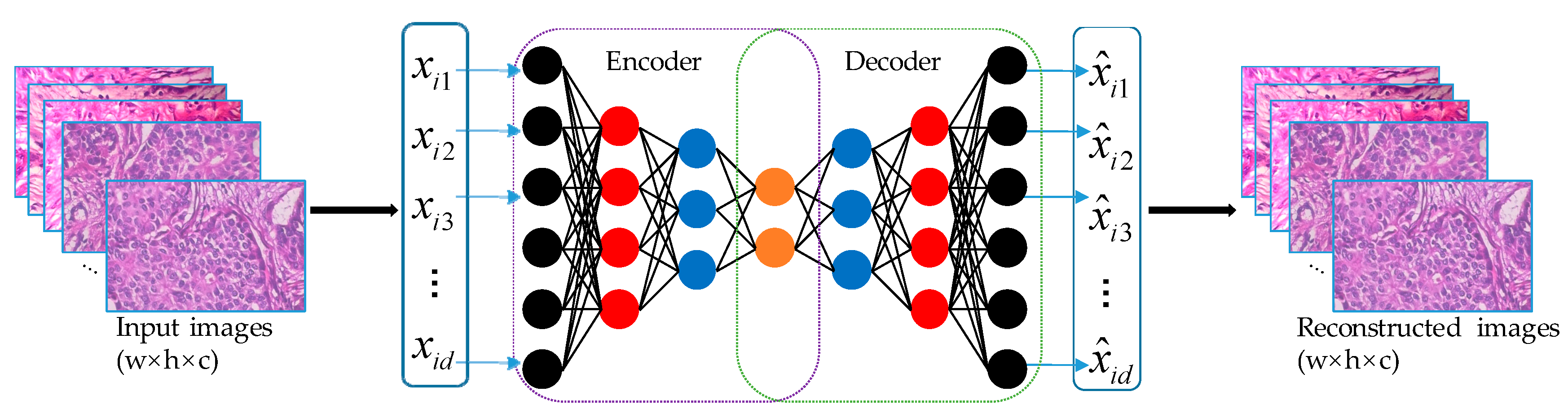
2.1.1. Autoencoder
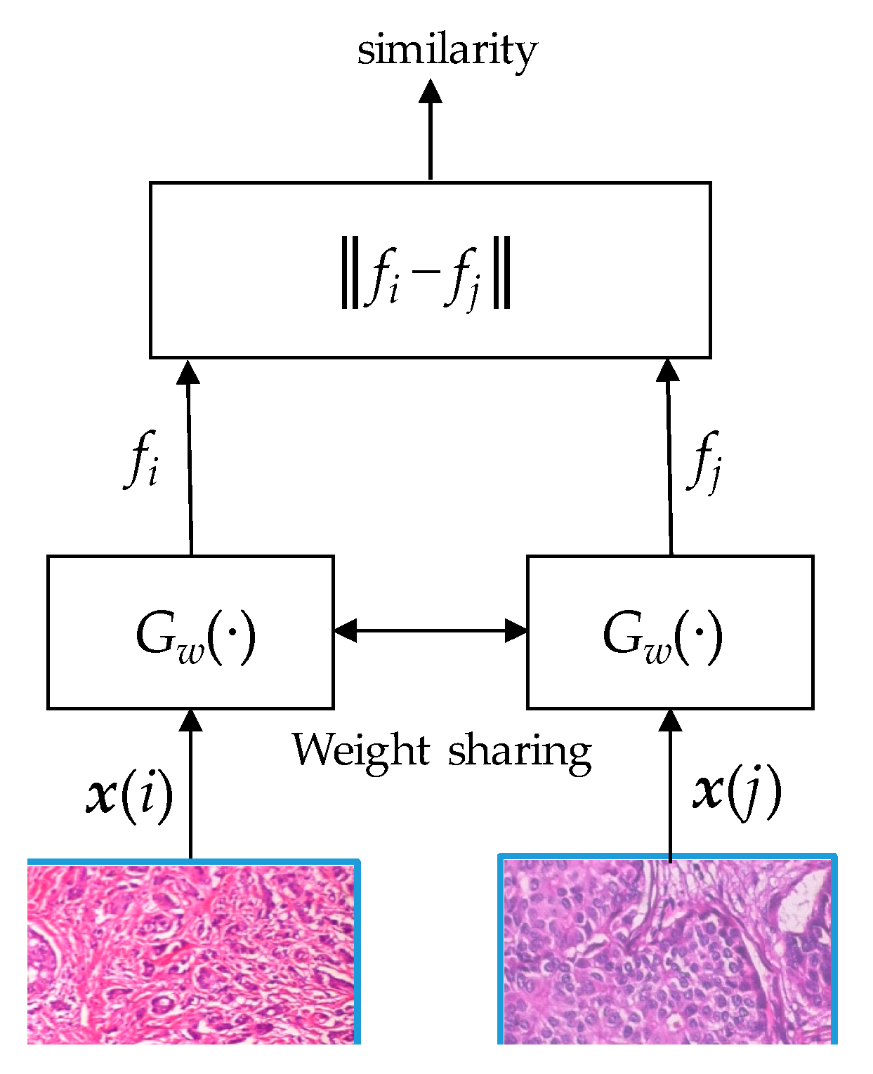
2.1.2. Siamese Network
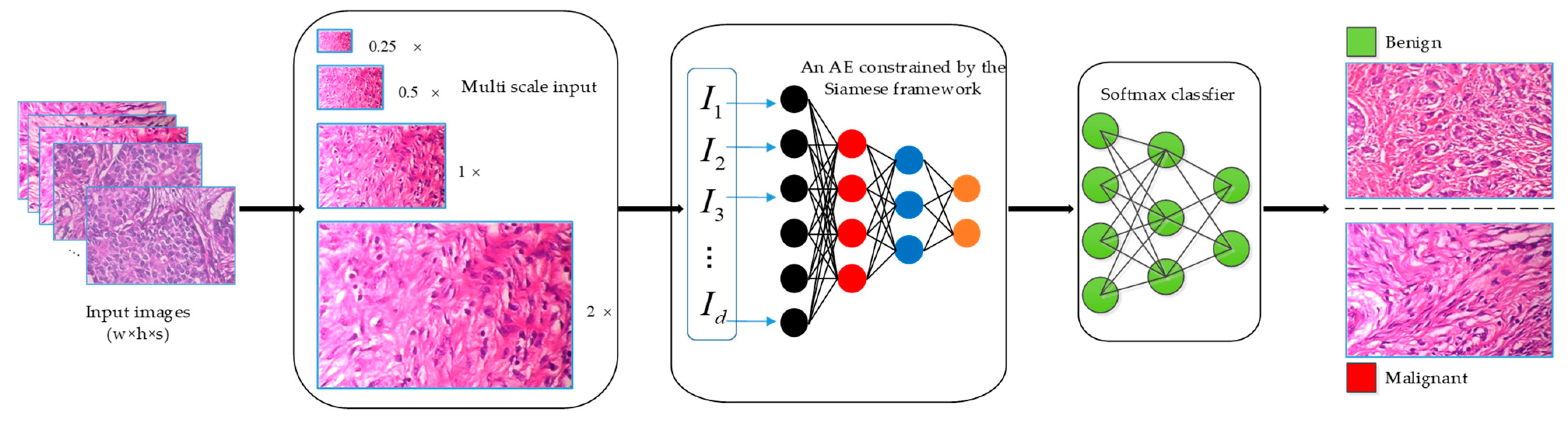
2.2. Proposed Approach
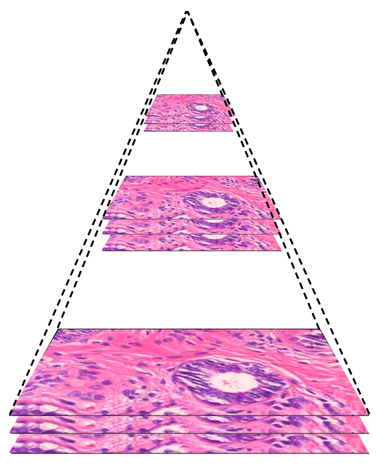
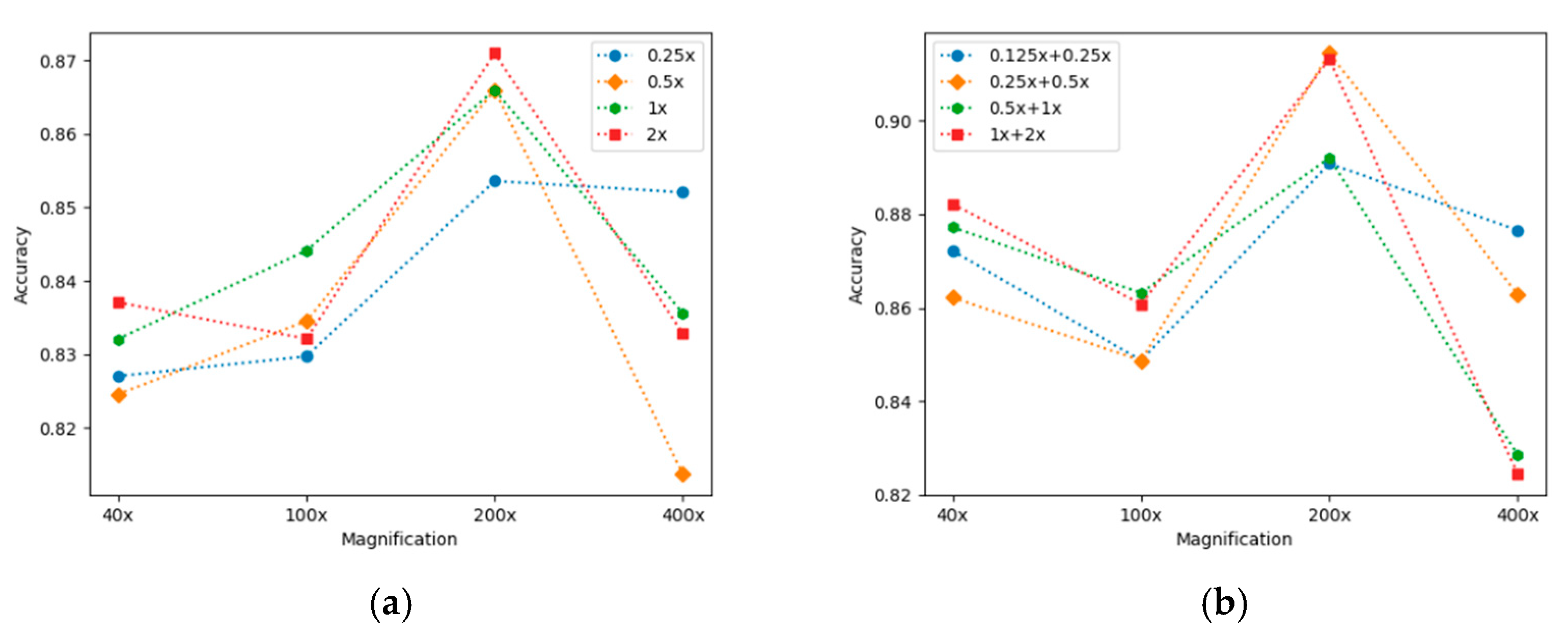
2.2.1. Multi-Scale Input
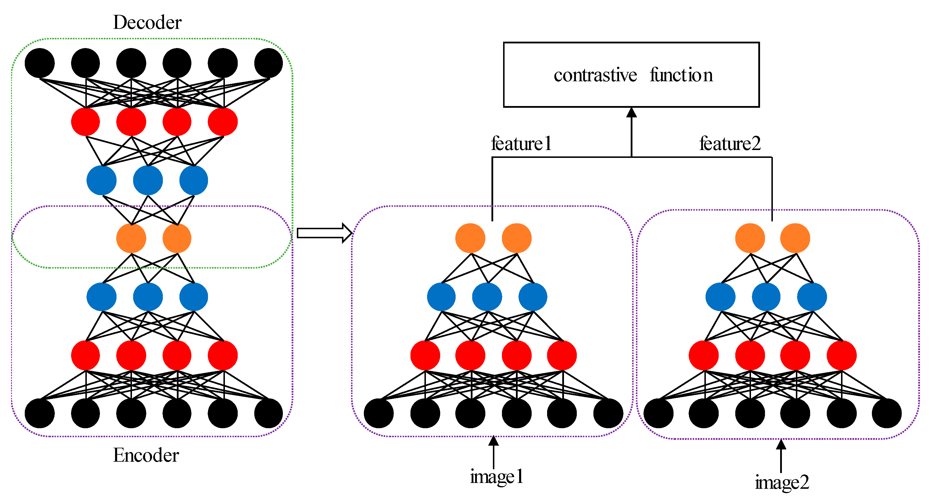
2.2.2. Siamese Framework Based on AE
2.2.3. Loss Function
| Algorithm 1. The training procedure for AE + Siamese Network. |
| Input: |
| The training set: ; learning rate: α; and iterative number: It. |
| Output: The weights and biases: |
| 1. Initialize according to the trained AE. 2. Build a Siamese network with two AE with shared weights. |
| 3. for each do |
| for each do Do forward propagation. End for for each do Fine-tune by minimizing loss function of Siamese network. End for End for 4. Return |
3. Results
3.1. BreakHis Dataset
3.2. Performence Metrics
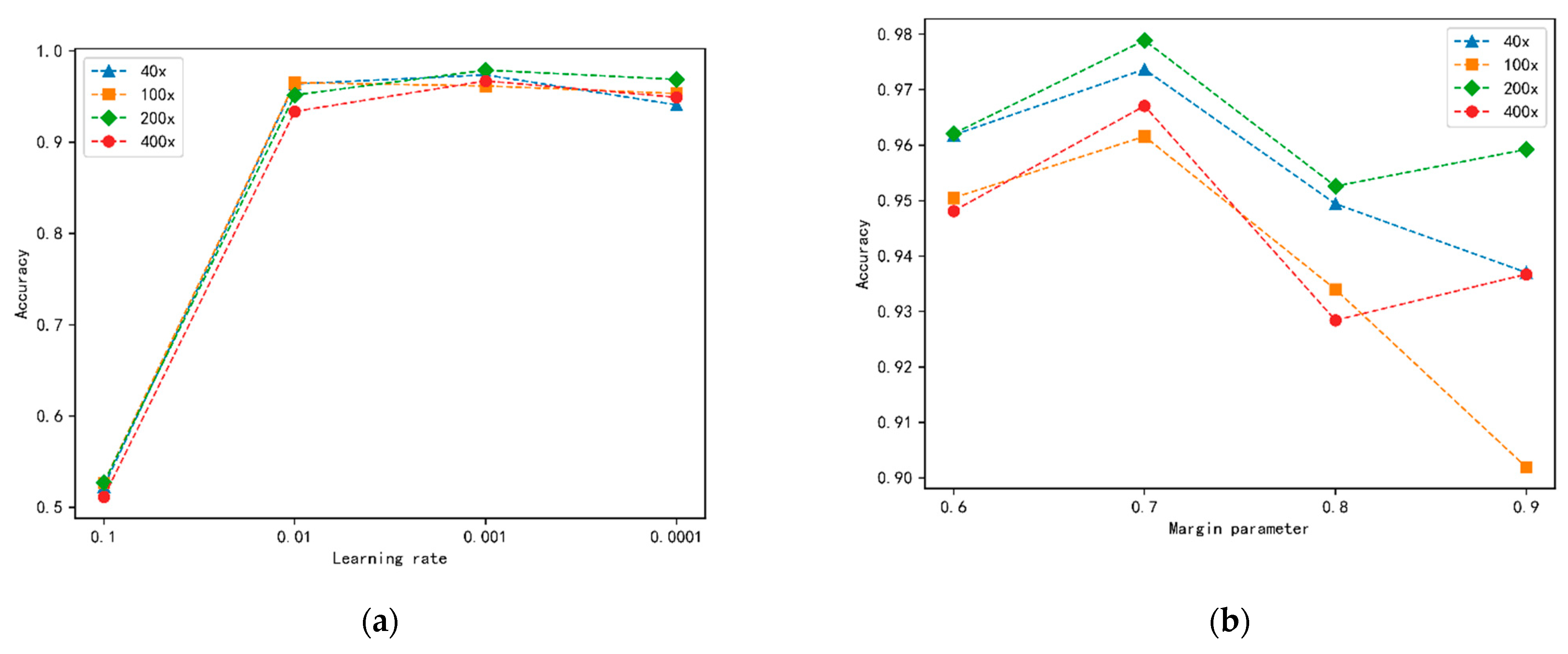
3.3. Experimental Settings
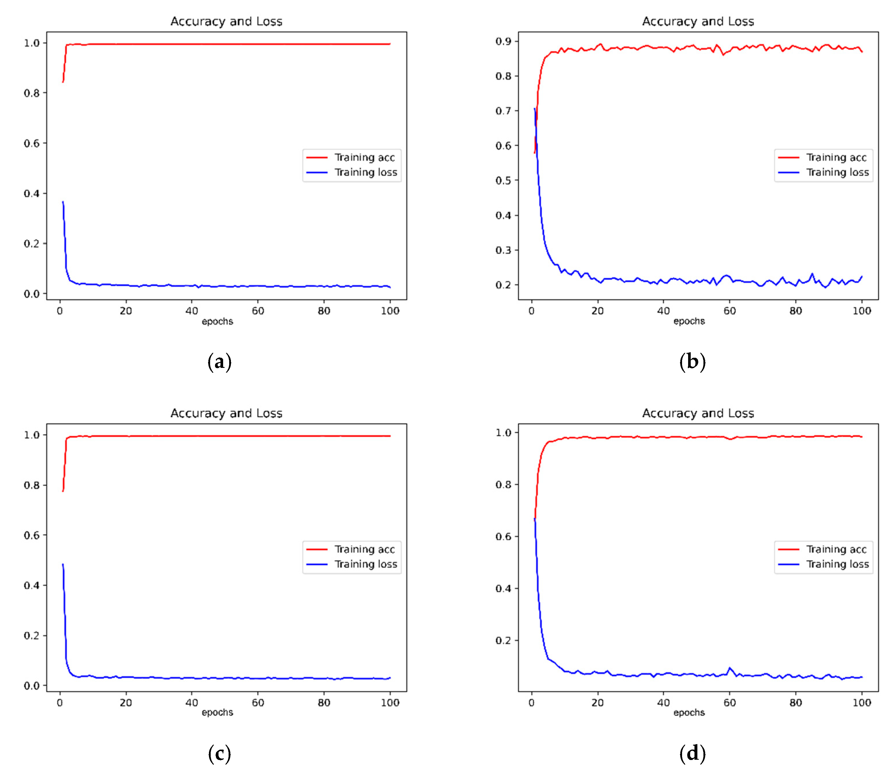
3.4. Results and Analysis
4. Discussion
5. Conclusions
Author Contributions
Funding
Institutional Review Board Statement
Informed Consent Statement
Data Availability Statement
Conflicts of Interest
References
- Sung, H.; Ferlay, J.; Siegel, R.L.; Laversanne, M.; Soerjomataram, I.; Jemal, A.; Bray, F. Global cancer statistics 2020: GLOBOCAN estimates of incidence and mortality worldwide for 36 cancers in 185 countries. CA Cancer J. Clin. 2021, 71, 209–249. [Google Scholar] [CrossRef] [PubMed]
- Al-antari, M.A.; Al-masni, M.A.; Park, S.U.; Park, J.; Metwally, M.K.; Kadah, Y.M.; Han, S.M.; Kim, T.S. An Automatic Computer-Aided Diagnosis System for Breast Cancer in Digital Mammograms via Deep Belief Network. J. Med. Biol. Eng. 2018, 38, 443–456. [Google Scholar] [CrossRef]
- Celaya-Padilla, J.M.; Guzmán-Valdivia, C.H.; Galván-Tejada, C.E.; Galván-Tejada, J.I.; Gamboa-Rosales, H.; Garza-Veloz, I.; Martinez-Fierro, M.L.; Cid-Báez, M.A.; Martinez-Torteya, A.; Martinez-Ruiz, F.J. Contralateral asymmetry for breast cancer detection: A CADx approach. J. Med. Biol. Eng. 2018, 38, 115–125. [Google Scholar] [CrossRef]
- Chan, H.P.; Samala, R.K.; Hadjiiski, L.M. CAD and AI for breast cancer—Recent Development and Challenges. Br. J. Radiol. 2019, 93, 1108. [Google Scholar] [CrossRef]
- Avanzo, M.; Porzio, M.; Lorenzon, L.; Milan, L.; Sghedoni, R.; Russo, G.; Massafra, R.; Fanizzi, A.; Barucci, A.; Ardu, V.; et al. Artificial intelligence applications in medical imaging: A review of the medical physics research in Italy. Phys. Med. 2021, 83, 221–241. [Google Scholar] [CrossRef] [PubMed]
- Massafra, R.; Bove, S.; Lorusso, V.; Biafora, A.; Comes, M.C.; Didonna, V.; Diotaiuti, S.; Fanizzi, A.; Nardone, A.; Nolasco, A.; et al. Radiomic Feature Reduction Approach to Predict Breast Cancer by Contrast-Enhanced Spectral Mammography Images. Diagnostics 2021, 11, 684. [Google Scholar] [CrossRef]
- Comes, M.C.; La Forgia, D.; Didonna, V.; Fanizzi, A.; Giotta, F.; Latorre, A.; Martinelli, E.; Mencattini, A.; Paradiso, A.V.; Tamborra, P.; et al. Early Prediction of Breast Cancer Recurrence for Patients Treated with Neoadjuvant Chemotherapy: A Transfer Learning Approach on DCE-MRIs. Cancers 2021, 13, 2298. [Google Scholar] [CrossRef]
- Krithiga, R.; Geetha, P. Breast Cancer Detection, Segmentation and Classification on Histopathology Images Analysis: A Systematic Review. Arch. Comput. Methods Eng. 2020, 10, 2607–2619. [Google Scholar] [CrossRef]
- Kowal, M.; Filipczuk, P.; Obuchowicz, A.; Korbicz, J.; Monczak, R. Computer-aided diagnosis of breast cancer based on fine needle biopsy microscopic images. Comput. Biol. Med. 2013, 43, 1563–1572. [Google Scholar] [CrossRef]
- George, Y.M.; Zayed, H.H.; Roushdy, M.I.; Elbagoury, B.M. Remote Computer-Aided Breast Cancer Detection and Diagnosis System Based on Cytological Images. IEEE Syst. J. 2014, 8, 949–964. [Google Scholar] [CrossRef]
- Filipczuk, P.; Fevens, T.; Krzyżak, A.; Monczak, R. Computer-Aided Breast Cancer Diagnosis Based on the Analysis of Cytological Images of Fine Needle Biopsies. IEEE Trans. Med. Imaging 2013, 32, 2169–2178. [Google Scholar] [CrossRef] [PubMed]
- Bayramoglu, N.; Kannala, J.; Heikkila, J. Deep learning for magnification independent breast cancer histopathology image classification. In Proceedings of the International Conference on Pattern Recognition (ICCV), Cancun, Mexico, 4–8 December 2016. [Google Scholar]
- Spanhol, F.A.; Oliveira, L.S.; Petitjean, C.; Heutte, L. Breast Cancer Histopathological Image Classification using Convolutional Neural Networks. In Proceedings of the International Joint Conference on Neural Networks (IJCNN), Vancouver, BC, Canada, 24–29 July 2016. [Google Scholar]
- Spanhol, F.A.; Oliveira, L.S.; Cavalin, P.R.; Petitjean, C.; Heutte, L. Deep features for breast cancer histopathological image classification. In Proceedings of the IEEE International Conference on Systems, Rome, Italy, 9–11 October 2017. [Google Scholar]
- Wang, Z.; Dong, N.; Dai, W.; Rosario, S.D.; Xing, E.P. Classification of breast cancer histopathological images using convolutional neural networks with hierarchical loss and global pooling. In Proceedings of the International Conference Image Analysis and Recognition (ICIAR), Póvoa de Varzim, Portugal, 27–29 June 2018. [Google Scholar]
- Brancati, N.; Frucci, M.; Riccio, D. Multi-classification of breast cancer histology images by using a fine-tuning strategy. In Proceedings of the International Conference Image Analysis and Recognition (ICIAR), Póvoa de Varzim, Portugal, 27–29 June 2018. [Google Scholar]
- Pimkin, A.; Makarchuk, G.; Kondratenko, V.; Pisov, M.; Krivov, E.; Belyaev, M. Ensembling neural networks for digital pathology images classification and segmentation. In Proceedings of the International Conference Image Analysis and Recognition (ICIAR), Póvoa de Varzim, Portugal, 27–29 June 2018. [Google Scholar]
- Wan, S.; Lee, H.C.; Huang, X.; Xu, T.; Xu, T.; Zeng, X.; Zhang, Z.; Sheikine, Y.; Connolly, J.L.; Fujimoto, J.G. Integrated local binary pattern texture features for classification of breast tissue imaged by optical coherence microscopy. Med. Image Anal. 2017, 38, 104–116. [Google Scholar] [CrossRef] [PubMed] [Green Version]
- Nanni, L.; Brahnam, S.; Lumini, A. A very high performing system to discriminate tissues in mammograms as benign and malignant. Expert Syst. Appl. 2012, 39, 1968–1971. [Google Scholar] [CrossRef]
- Sharma, M.; Singh, R.; Bhattacharya, M. Classification of breast tumors as benign and malignant using textural feature descriptor. In Proceedings of the IEEE International Conference on Bioinformatics & Biomedicine, Kansas City, MO, USA, 13–16 November 2017. [Google Scholar]
- Gupta, V.; Bhavsar, A. Breast Cancer Histopathological Image Classification: Is Magnification Important? In Proceedings of the IEEE Conference on Computer Vision and Pattern Recognition Workshops (CVPRW), Honolulu, HI, USA, 21–26 July 2017. [Google Scholar]
- Feng, Y.; Lei, Z.; Mo, J. Deep Manifold Preserving Autoencoder for Classifying Breast Cancer Histopathological Images. IEEE/ACM Trans. Comput. Biol. Bioinform. 2020, 17, 91–101. [Google Scholar] [CrossRef]
- Alom, M.Z.; Yakopcic, C.; Nasrin, M.S.; Taha, T.M.; Asari, V.K. Breast cancer classification from histopathological images with inception recurrent residual convolutional neural network. J. Digit. Imaging 2019, 32, 605–617. [Google Scholar] [CrossRef] [Green Version]
- Sudharshan, P.J.; Petitjean, C.; Spanhol, F.; Oliveira, L.E.; Heutte, L.; Honeine, P. Multiple instance learning for histopathological breast cancer image classification. Expert Syst. Appl. 2019, 117, 103–111. [Google Scholar] [CrossRef]
- Yan, R.; Ren, F.; Wang, Z.; Wang, L.; Zhang, T.; Liu, Y.; Rao, X.; Zheng, C.; Zhang, F. Breast cancer histopathological image classification using a hybrid deep neural network. Methods 2020, 173, 52–60. [Google Scholar] [CrossRef]
- Sheikh, T.S.; Lee, Y.; Cho, M. Histopathological Classification of Breast Cancer Images Using a Multi-Scale Input and Multi-Feature Network. Cancers 2020, 12, 2031. [Google Scholar] [CrossRef]
- Comes, M.C.; Filippi, J.; Mencattini, A.; Casti, P.; Cerrato, G.; Sauvat, A.; Vacchelli, E.; De Ninno, A.; Di Giuseppe, D.; D’Orazio, M.; et al. Multi-scale gener-active adversarial network for improved evaluation of cell—Cell interactions served in organ-on-chip experiments. Neural. Comput. Appl. 2021, 8, 3671–3689. [Google Scholar] [CrossRef]
- Bromley, J.; Bentz, J.W.; Bottou, L.; Guyon, I.; LeCun, Y.; Moore, C.; Sackinger, E.; Shah, R. Signature verification using a “siamese” time delay neural network. Int. J. Pattern Recognit. Artif. 1993, 7, 669–688. [Google Scholar] [CrossRef] [Green Version]
- Kallenberg, M.; Petersen, K.; Nielsen, M.; Ng, A.Y.; Diao, P.; Igel, C.; Vachon, C.M.; Holland, K.; Winkel, R.R.; Karssemeijer, N. Unsupervised deep learning applied to breast density segmentation and mammographic risk scoring. IEEE Trans. Med. Imaging 2016, 35, 1322–1331. [Google Scholar] [CrossRef] [PubMed]
- Li, X.; Shen, X.; Zhou, Y.; Wang, X.; Li, T.Q. Classification of breast cancer histopathological images using interleaved DenseNet with SENet (IDSNet). PLoS ONE 2020, 15, e0232127. [Google Scholar] [CrossRef] [PubMed]
- Kumar, A.; Singh, S.K.; Saxena, S.; Lakshmanan, K.; Sangaiah, A.K.; Chauhan, H.; Shrivastava, S.; Singh, R.K. Deep feature learning for histopathological image classification of canine mammary tumors and human breast cancer. Inf. Sci. 2020, 508, 405–421. [Google Scholar] [CrossRef]
- Budak, Ü.; Cömert, Z.; Rashid, Z.N.; Şengür, A.; Çıbuk, M. Computer-aided diagnosis system combining FCN and Bi-LSTM model for efficient breast cancer detection from histopathological images. Appl. Soft Comput. 2019, 85, 105765. [Google Scholar] [CrossRef]
- Spanhol, F.A.; Oliveira, L.S.; Petitjean, C.; Heutte, L. A dataset for breast cancer histopathological image classification. IEEE Trans. Biomed. Eng. 2015, 63, 1455–1462. [Google Scholar] [CrossRef]


| Magnification | Benign | Malignant | Total |
|---|---|---|---|
| 40× | 625 | 1370 | 1995 |
| 100× | 644 | 1437 | 2081 |
| 200× | 623 | 1390 | 2013 |
| 400× | 588 | 1232 | 1820 |
| total | 2480 | 5429 | 7909 |
| patient | 24 | 58 | 82 |
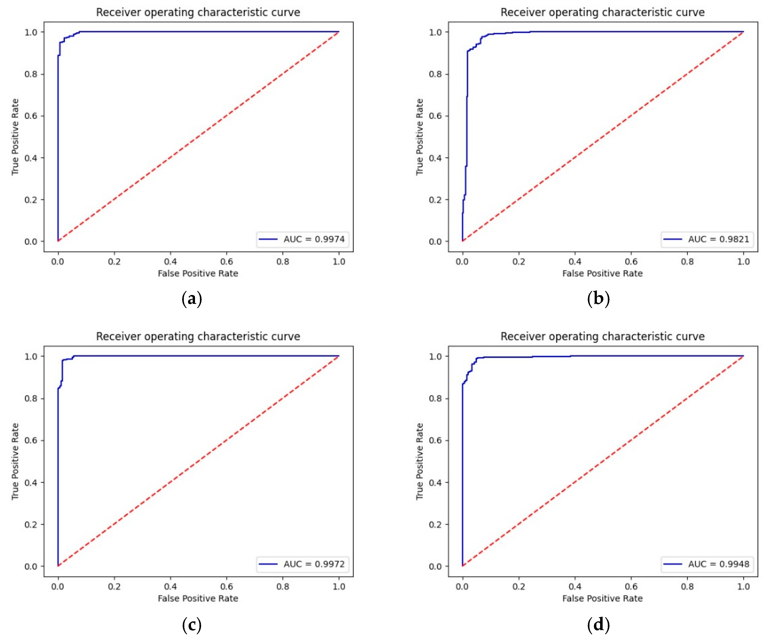
| (a). 40× magnification. | ||||
| Methods | Accuracy | Precision | Recall | Specificity |
| AE + SoftMax | 88.2 | 88.6 | 95.0 | 73.2 |
| AE + Siamese Network | 97.3 | 96.9 | 99.2 | 93.2 |
| (b). 100× magnification | ||||
| Methods | Accuracy | Precision | Recall | Specificity |
| AE + SoftMax | 86.3 | 86.8 | 94.4 | 68.2 |
| AE + Siamese Network | 96.1 | 95.7 | 98.7 | 90.3 |
| (c). 200× magnification. | ||||
| Methods | Accuracy | Precision | Recall | Specificity |
| AE + SoftMax | 91.4 | 92.3 | 95.5 | 82.4 |
| AE + Siamese Network | 97.8 | 97.6 | 99.2 | 94.8 |
| (d). 400× magnification. | ||||
| Methods | Accuracy | Precision | Recall | Specificity |
| AE + SoftMax | 87.6 | 89.1 | 93.1 | 76.2 |
| AE + Siamese Network | 96.7 | 95.7 | 99.5 | 90.6 |
| (a). 40× magnification. | |||||
| Methods | Accuracy | Precision | Recall | F1-score | Time (s) |
| PFTAS + QDA [33] | 83.8 | - | - | - | - |
| PFTAS + SVM [33] | 81.6 | - | - | - | - |
| PFTAS + RF [33] | 81.8 | - | - | - | - |
| Inception_v3 | 73.4 | 79.5 | 82.4 | 81.0 | 1003.0 |
| Resnet50 | 79.1 | 77.5 | 98.1 | 86.6 | 3264.1 |
| Inception_resnet_v2 | 77.9 | 81.6 | 87.5 | 84.4 | 2123.5 |
| Xception | 79.9 | 79.9 | 94.8 | 86.7 | 2346.8 |
| IDSNet [30] | 89.1 | - | - | - | - |
| FE-VGGNET16-SVM(POLY) [31] | 94.1 | - | - | - | - |
| FCN-Bi-LSTM [32] | 95.6 | - | - | - | - |
| AE + Siamese Network | 97.3 | 96.9 | 99.2 | 98.1 | 320.6 |
| (b). 100× magnification. | |||||
| Methods | Accuracy | Precision | Recall | F1-score | Time (s) |
| PFTAS + QDA [33] | 82.1 | - | - | - | - |
| PFTAS + SVM [33] | 79.9 | - | - | - | - |
| PFTAS + RF [33] | 81.3 | - | - | - | - |
| Inception_v3 | 76.4 | 94.8 | 69.7 | 80.4 | 1063.7 |
| Resnet50 | 71.2 | 72.8 | 93.0 | 81.7 | 3422.8 |
| Inception_resnet_v2 | 70.0 | 90.9 | 62.8 | 74.2 | 2215.4 |
| Xception | 82.4 | 89.6 | 84.3 | 86.9 | 2445.8 |
| IDSNet [30] | 85.0 | - | - | - | - |
| FE-VGGNET16-SVM(POLY) [31] | 95.1 | - | - | - | - |
| FCN-Bi-LSTM [32] | 93.6 | - | - | - | - |
| AE + Siamese Network | 96.1 | 95.7 | 98.7 | 97.2 | 353.6 |
| (c). 200× magnification. | |||||
| Methods | Accuracy | Precision | Recall | F1-score | Time (s) |
| PFTAS + QDA [33] | 84.2 | - | - | - | - |
| PFTAS + SVM [33] | 85.1 | - | - | - | - |
| PFTAS + RF [33] | 83.5 | - | - | - | - |
| Inception_v3 | 86.6 | 95.9 | 84.1 | 89.6 | 1083.7 |
| Resnet50 | 89.3 | 91.2 | 93.5 | 92.3 | 3307.6 |
| Inception_resnet_v2 | 80.8 | 92.7 | 78.4 | 84.9 | 2167.4 |
| Xception | 92.3 | 90.7 | 98.9 | 94.6 | 2377.2 |
| IDSNet [30] | 87.0 | - | - | - | - |
| FE-VGGNET16-SVM(POLY) [31] | 97.0 | - | - | - | - |
| FCN-Bi-LSTM [32] | 96.3 | - | - | - | - |
| AE + Siamese Network | 97.8 | 97.6 | 99.2 | 98.4 | 347.4 |
| (d). 400× magnification. | |||||
| Methods | Accuracy | Precision | Recall | F1-score | Time (s) |
| PFTAS + QDA [33] | 82.0 | - | - | - | - |
| PFTAS + SVM [33] | 82.3 | - | - | - | - |
| PFTAS + RF [33] | 81.0 | - | - | - | - |
| Inception_v3 | 91.5 | 92.5 | 95.1 | 93.8 | 911.9 |
| Resnet50 | 72.6 | 71.6 | 98.3 | 82.9 | 2997.4 |
| Inception_resnet_v2 | 83.8 | 85.6 | 91.4 | 88.4 | 3818.8 |
| Xception | 86.8 | 89.9 | 90.6 | 90.3 | 1967.9 |
| IDSNet [30] | 84.5 | - | - | - | - |
| FE-VGGNET16-SVM(POLY) [31] | 93.4 | - | - | - | - |
| FCN-Bi-LSTM [32] | 94.2 | - | - | - | - |
| AE + Siamese Network | 96.7 | 95.7 | 99.5 | 97.6 | 318.1 |
Publisher’s Note: MDPI stays neutral with regard to jurisdictional claims in published maps and institutional affiliations. |
© 2022 by the authors. Licensee MDPI, Basel, Switzerland. This article is an open access article distributed under the terms and conditions of the Creative Commons Attribution (CC BY) license (https://creativecommons.org/licenses/by/4.0/).
Share and Cite
Liu, M.; He, Y.; Wu, M.; Zeng, C. Breast Histopathological Image Classification Method Based on Autoencoder and Siamese Framework. Information 2022, 13, 107. https://doi.org/10.3390/info13030107
Liu M, He Y, Wu M, Zeng C. Breast Histopathological Image Classification Method Based on Autoencoder and Siamese Framework. Information. 2022; 13(3):107. https://doi.org/10.3390/info13030107
Chicago/Turabian StyleLiu, Min, Yu He, Minghu Wu, and Chunyan Zeng. 2022. "Breast Histopathological Image Classification Method Based on Autoencoder and Siamese Framework" Information 13, no. 3: 107. https://doi.org/10.3390/info13030107