Study on Hydrodynamic Characteristics and Environmental Response in Shantou Offshore Area

Abstract

As a coastal trading city in China, Shantou has complex terrain and changeable sea conditions in its coastal waters. In order to better protect the coastal engineering and social property along the coast, based on the numerical simulation method, this paper constructed a detailed hydrodynamic model of the Shantou sea area, and the measured tide elevation and tidal current were used to verify the accuracy of the model. Based on the simulation results, the tide elevation and current in the study area were analyzed, including the flood and ebb tides of astronomical spring tide, the flood and ebb tides of astronomical neap tide, the high tide, and the low tide. In order to find the main tidal constituent types in this sea, the influence of different tidal constituents on tide elevation and tidal current in the study area was analyzed. At the same time, the storm surge model of the study area was constructed, and the flow field under Typhoon “Mangkhut” in the study area was simulated by using the real recorded data. Typhoon wind fields with different recurrence periods and intensities were constructed to simulate the change in the flow field, the sea water level, and the disaster situation along the coast. The results showed that under normal sea conditions, the sea water flows from southwest to northeast at flood tide and the flow direction is opposite at ebb tide. The tidal range is large in the northwest and small in the southeast of the study area. The tides in the study area are mainly controlled by M2, S2, K1, and O1 tidal constituents, but N2, K2, P1, and Q1 tidal constituents have significant effects on the high water level. The water level caused by typhoons increases significantly along the coast of Shantou City. In the west area of the Rong River estuary, a typhoon with a lower central pressure than 910 hPa may induce a water increase of more than 2 m.

1. Introduction

Shantou City, located on the golden position of Hong Kong and Southeast Asia, is an important node of the Maritime Silk Road. Shantou City faces the Taiwan Province Strait to the east, 214 nautical miles away from Kaohsiung Port and 187 nautical miles away from Hong Kong. At the same time, Shantou Port is located in the downtown area of Shantou. It is one of the 25 major coastal hub ports recognized by the Ministry of Transport of the People’s Republic of China and the five major ports in Guangdong Province.

In order to ensure the production and life of Shantou coastal waters, the Shantou Marine Hydrological Weather Bureau has carried out relevant investigations. The survey showed that the hydrological and climatic conditions of Shantou and its coastal areas are complicated, with tortuous shorelines, rivers entering the sea, and a dense distribution of complex movement of seawater in some years. The changing tidal current affects the life of the people in Shantou city and the operation of ships in Shantou Port. Coastal cities also suffer from marine disasters such as typhoon storm surges and tsunamis [1]. Typhoons may lead to serious water increases and storm surges. Since 1949, many typhoons have occurred in Shantou, causing serious disasters. For example, in 1969, Typhoon “Viola” caused the water level to rise by more than one meter, killing 956 people and destroying 93,000 square kilometers of farmland. In 1979, Typhoon “Hope” killed 93 people, and destroyed more than 20,000 houses and 60,000 hectares of farmland. In 1986, Typhoon “Peggy” inundated 586,000 hectares of farmland, killed 206 people, sank 64 boats, and destroyed more than 81,000 houses. According to statistics, 201 tropical cyclones entered Shantou from 1950 to 2012. On average, there are 3.2 tropical cyclones every year. Among them, the tropical cyclones entering Shantou are mostly typhoons and severe tropical storms, accounting for 65% of the total. These typhoon paths are divided into five categories: landing from the west, landing from the front, landing from the east, passing by land, and passing by sea. About 60% of typhoons belong to the first two categories, and 35% of typhoons are landing from the east [2]. It can be seen that extreme weather does great harm to Shantou City. Generally speaking, the hydrodynamic conditions in the Shantou coastal area are complex and vulnerable to typhoons [3,4,5]. Therefore, in order to guarantee safety for the production and life of the port and coast, it is extremely necessary to establish a fine marine water environment dynamic simulation model in Shantou City. In this way, a hydrodynamic simulation of Shantou City can be carried out to better understand the tidal current in this sea area. On this basis, typhoon simulations can help us understand the disaster caused by typhoon storm surges, to provide a scientific basis for disaster prevention and mitigation.

Compared with the traditional observation and acquisition, the use of numerical simulation is more efficient and more cost-effective [6,7]. By means of numerical simulation, we can better understand the distribution of tidal current in the Shantou sea area and the damage of storm surges. Numerical simulation technology has been applied well to the simulation of sea water movement and marine disasters. For example, Lai et al. [8] used FVCOM to simulate the circulation in the Pearl River Estuary and reproduce the observation characteristics of ocean currents. Liu et al. [9] studied the abnormal water increase in the Pearl River Estuary area caused by storm surges from Typhoon “Hato” through the numerical simulation of sea water movement. Xu et al. [10] analyzed the hydrodynamic characteristics and silt backfill in the channel in the western port area of Shenzhen Port through numerical simulation using a mathematical model. Jia et al. [11] established a two-dimensional hydrodynamic model of the Wanbao Lake based on MIKE21, and analyzed the dynamic characteristics of the lake and pollutant migration.

In this paper, a detailed hydrodynamic model of the Shantou offshore area was established on the basis of existing research. The accuracy of the model was verified by comparing the measured ocean current data with the tide station water level. The simulated sea area was about 4 × 10³ km², mainly including the sea area in the southeast of Shantou City with a water depth of less than 30 m (Figure 1). At the same time, the variations in sea water level and flow field in the study area were given. The variation in sea water flow field under different tidal currents and the distributions of water level and flow velocity under different wind conditions were discussed. In the Section 2, the model is introduced and verified. The Section 3 discusses the characteristics of the flow field in the study area at different times and the effects of different tidal constituents and wind fields on the results. The Section 4 includes the conclusions.

2. Model Introduction and Verification

2.1. The Information of Data Used

The data used in the model included shoreline data, topographic water depth data, open boundary forced water level data, wind field data, and river discharge data.

The original shoreline data of the study area were obtained from the Global Self-consistent, Hierarchial, High-Resolution Geography Database. Geodas software was used for extraction. Chart (NO. 81001) and remote sensing images were used to adjust details.

The open sea area topographic data of the model were obtained from National Oceanic and Atmospheric Administration’s ETOPO1 data. ETOPO1 data represent a 1 arc-minute global relief model of Earth’s surface that integrates land topography and ocean bathymetry, while the offshore topographic data were extracted from charts.

The open boundary forced water level data came from the data calculated by TPXO 2016. TPXO (Topex/Poseidon Crossover Solution) is a global tidal inversion model established by Oregon State University with T/P intersection data.

The discharge data of Hanjiang River and Rongjiang River came from the measured data of Chaoan hydrological observation station and Dongqiaoyuan hydrological observation station.

Wind field data were from the European Centre for Medium-Range Weather Forecasts. The resolution of wind field was 1/8° × 1/8° (https://cds.climate.copernicus.eu (accessed on 15 July 2020)).

2.2. Introduction to the Model Used

Using numerical models is a good way to study the water. Numerical simulation has been widely used in the study of the flow field of rivers, lakes, oceans, around coastal engineering, and so on [12,13,14,15].

The governing equation of the model is as follows:

$$\frac{\partial \zeta }{\partial t}\hspace{0.17em}+\hspace{0.17em}\frac{\partial (Hu)}{\partial x}\hspace{0.17em}+\hspace{0.17em}\frac{\partial (Hv)}{\partial y}\hspace{0.17em}=\hspace{0.17em}0$$

(1)

$$\frac{\partial u}{\partial t}+u\frac{\partial u}{\partial x}+v\frac{\partial u}{\partial y}=F_x+c_{f}v-g\frac{\partial \zeta }{\partial x}-gu\frac{\sqrt{u^2+v^2}}{C^{2}H}+\mu \left(\frac{{\partial }^{2}u}{\partial x^2}+\frac{{\partial }^{2}u}{\partial y^2}\right)-\frac{1}{{\rho }_0}\frac{\partial P_a}{\partial x}$$

(2)

$$\frac{\partial v}{\partial t}+u\frac{\partial v}{\partial x}+v\frac{\partial v}{\partial y}=F_y+c_{f}u-g\frac{\partial \zeta }{\partial y}-gv\frac{\sqrt{u^2+v^2}}{C^{2}H}+\mu \left(\frac{{\partial }^{2}v}{\partial x^2}+\frac{{\partial }^{2}v}{\partial y^2}\right)-\frac{1}{{\rho }_0}\frac{\partial P_a}{\partial y}$$

(3)

$$\overline{{\tau }_s}={\rho }_a{c}_d\left|\overline{u_w}\right|\overline{u_w}$$

(4)

Equation (1) represents the continuity equation, where $\zeta$ is the water level, t is time, H is water depth, x and y are coordinates in the Cartesian coordinate system, and u and v are the average velocity components along the water depth in the x and y directions, respectively. Equations (2) and (3) represent the conservation of momentum in the x and y directions, respectively, where F_x and F_y are source and sink items in the x and y directions, respectively, c_f is the Coriolis force, g is gravitational acceleration, C is the Schetze coefficient, $\mu$ is the viscous force coefficient, ${\rho }_0$ is the fluid density, and Pa is atmospheric pressure. Equation (4) is the calculation formula for the surface stress of the wind field, ${\rho }_a$ is the air density, $\overline{u_w}$ is the wind speed at 10 m high, and c_d is the drag coefficient of wind stress [16]. According to Wu’s [17] empirical formula, when the wind speed is less than 25 ms⁻¹, c_d is 0.001255; when the wind speed is larger than 25 ms⁻¹, c_d is 0.002425.

It is necessary to add fixed boundary conditions and initial conditions to make the model have unique solutions. The initial conditions and boundary conditions are shown in the following equation:

$$\begin{array}{l}{\zeta (x,y)|}_{t=0}={\zeta }_0(x,y)\\ {p(x,y)|}_{t=0}=p_0(x,y)\\ {q(x,y)|}_{t=0}=q_0(x,y)\end{array}$$

(5)

$$C{(x,y,t)}^{}{=}^{}{C}^{*}(x,y,t)$$

(6)

$$V_n=0$$

(7)

Equation (5) is the initial condition equation. Equation (6) is the open boundary condition, where $C^{*}(x,y,t)$ are artificial set conditions (e.g., water level, flow velocity, and discharge) at an open boundary. Equation (7) is the land boundary condition, where n is the normal direction of the land boundary and V_n is the water velocity in the normal direction at land borders.

2.3. Model Setup

The study area is divided by a triangular unstructured grid (Figure 2). The grid gradually becomes densified from the sea to the shoreline. The grid resolution of the nearshore part is 150 m, and that of the sea boundary part is 5000 m. There are a total of 58,444 grid nodes in the whole area. The study area is divided into 113,148 triangular grids.

In the model, the normal velocity of sea flow at the land boundary is zero. The water level at the open boundary is calculated by the TPXO model. The water level is controlled by astronomical tides. To be more specific, the water level at the open boundary is calculated by taking into account 8 tidal constituents, which are M2, S2, K1, O1, N2, K2, P1, and Q1. The discharge data of Hanjiang River and Rongjiang River were used as input conditions in the model. At the same time, the meteorological data provided by ECMWF were input into the model as wind field conditions. The simulation period was from 1 June 2020 to 30 June 2020. The minimum time step of the model was 0.01 s and the maximum time step was 30 s. The eddy viscosity coefficient is given by the Smagorinsky formula and the value is 0.28 [18]. The bed resistance used the Manning number, which is 32 m^1/3/s.

In fact, some baroclinic conditions such as thermohaline can also affect the whole hydrodynamic process [19]. Zhao et al. [20] used the POM, which is a baroclinic model, to calculate the tidal energy of Beibu Gulf. However, the focus of this study was the sea level and storm surges caused by typhoons. Compared to thermohaline, tides and wind play a more important role in contributing to the research focus. At the same time, the barotropic model has already had a good agreement with measurements, which can be used in the subsequent simulation (see Section 2.4). Thus, the density of seawater was set at a constant 1.05 kgm⁻³ and does not vary with temperature or salinity in this model.

Table 1. Parameter setting of each experiment.

	Astronomical Tidal Boundary	Wind Field	Time	Other Conditions
Experiment for model validation (Section 2.4)	M2, S2, K1, O1, N2, K2, P1, Q1	normal wind	6-1 0:00–7-1 0:00	remain the same as model setup
Experiment for astronomic tide (Section 3.1)	M2, S2, K1, O1, N2, K2, P1, Q1	normal wind	6-1 0:00–7-1 0:00	remain the same as model setup
Experiment for tidal constituent (Section 3.2)	M2, S2, K1, O1	normal wind	6-1 0:00–6-16 0:00	remain the same as model setup
Experiment for tidal constituent (Section 3.2)	M2, S2, K1, O1, P1	normal wind	6-1 0:00–6-16 0:00	remain the same as model setup
Experiment for Typhoon “Mangokhut” (Section 3.3)	M2, S2, K1, O1, N2, K2, P1, Q1	wind field of typhoon “Mangkhut”	6-11 0:00–6-15 0:00	remain the same as model setup
Experiment of typhoon in different recurrence periods (Section 3.3)	M2, S2, K1, O1, N2, K2, P1, Q1	wind field calculated according to the formula	6-6 0:00–6-9 0:00	remain the same as model setup

shows the parameter setting of each experiment in the following paper.

2.4. Model Validation

In order to verify the accuracy of the model, the data of three tide stations in the surrounding waters of Shantou City were selected, and the tidal current was measured in three different positions by ship. The water level data are the measured data of the tide station. The tidal flow velocity and direction are the measured data of ADCP. The ADCP used was Aquadopp Profiler 600 kHz. The absolute error was ±0.5 cms⁻¹, and the relative error was ±1%. The positions of tide stations and ADCP points are shown in Figure 1. See

Table 2. Information of tide stations and ADCP points.

Station	Location	Observation Time
Yunaowan tide station	117°06′ E, 23°24′ N	6-6 00:00–6-30 23:00
Shantou tide station	116°44′ E, 23°20′ N
Haimen tide station	116°37′ E, 23°11′ N
ADCP point 1	116°52′ E, 23°08′ N	6-10 10:00–6-11 11:00
ADCP point 2	116°56′ E, 23°22′ N	6-11 13:00–6-12 14:00
ADCP point 3	116°41′ E, 23°06′ N	6-12 17:00–6-13 18:00

for detailed information.

The model data were compared with the measured tide levels of the three tide stations. The temporal resolution of measured tide level data provided by the three tide stations was once an hour. 1 June to 5 June was the span time of the model. The remaining 25 days were used for verification. The results are shown in Figure 3.

Figure 3 shows the comparison between the measured tide level and the model data. It can be found from the tide changes at the three tide stations that there are two unequal high tides and low tides in the study area within a day. Figure 3a shows the verification between the measured tide level and the model results of the Yunaowan tide station. The Yunaowan tide station is located in the southeast of Nan’ao Island, which is in the northwest of the study area. The average tide level in June here is about −0.03 m. The average tide level in June of the model is close to 0 m. According to the measured tide level in Yunaowan tide station, the maximum tidal range here is close to 2.5 m during the spring tide, while the tidal range is less than 1 m during the neap tide. It can be calculated that the average absolute error of the tide level in the model at Yunaowan tide station is 6.65 cm. Figure 3b is the verification of the measured tide level and the model results at Shantou tide station. Shantou tide station is located near Shantou Port and in the mouth of Rongjiang River. According to the measured water level of Shantou tide station, the average tide level here is −0.02 m, while the average tide level of the model results here is 0.03 m. According to the measured tide level of Shantou tide station, the tidal range of Shantou tide station is close to 1.8 m during the spring tide. The tidal range is about 0.8 m during the neap tide. The mean absolute error of the tide level in the model at Shantou station is 7.11 cm. Figure 3c shows the verification between the measured tide level and the model results of Haimen tide station. Haimen tide station is located near the southwest of the study area. According to the measured tide level, the average tide level here is about −0.02 m, while the average tide level of the model results is 0 m. According to the measured water level data of Haimen tide station, the tidal range of Haimen tide station is about 1.7 m during the neap tide. The tidal range is about 0.6 m during the neap tide. According to the calculation, the mean absolute error of tide level in the model at Haimen tide station is 4.05 cm. The comparison between the model and the measured tide level of the three tide stations shows that the model is in good agreement with the measured data. The mean absolute errors of the three locations are 6.65 cm, 7.11 cm, and 4.05 cm, respectively.

The observation time of sea current at each place is 25 h. This covers a complete lunar day. The velocity verification is shown in Figure 4 and the direction verification is shown in Figure 5.

Figure 4 shows the verification between the measured velocity of ADCP and the simulated velocity by the model. The velocity of seawater is affected by many factors, such as tide, wind, and even passing ships. Figure 4a shows the verification result at ADCP point 1. This point is more than 20 km away from the land and nearly 30 m deep. The observation time is from 10:00 on 10 June 2020 to 11:00 on 11 June 2020. ADCP point 1 is located in the sea far away from the land. There are few islands around it, so the sea water flows smoothly here. During the observation period, the sea water flow velocity here is 0.30 ms⁻¹ on average, and up to 0.6 ms⁻¹ at flood tide and ebb tide. The sea water is slow at flat tide with the velocity being less than 0.01 ms⁻¹. Figure 4b is the verification result at ADCP point 2. This point is located at about 7 km on the south side of Nan’ao Island with a water depth of about 10 m. The observation time is from 13:00 on 11 June 2020 to 14:00 on 12 June 2020. ADCP point 2 is relatively close to the land. The water depth here is shallow, so the sea water here is more likely to be hindered by the terrain and the friction of the seabed. The sea water velocity here is slow. The average velocity is 0.13 ms⁻¹. The maximum velocity here is only 0.2 ms⁻¹. Figure 4c shows the verification result at ADCP point 3. ADCP point 3 is similar to ADCP point 1. It is located on the open sea, but closer to the land than ADCP point 1 is. The water depth at this point is about 20 m. The average sea water velocity here is 0.26 ms⁻¹. The velocity of sea water at ebb tide is smaller than that at flood tide. The maximum velocity of sea water at ebb tide is 0.32 ms⁻¹, while it can reach 0.59 ms⁻¹ at flood tide.

Figure 5a shows the flow direction at ADCP point 1. At the time of flood tide and ebb tide, the flow direction of the tidal current is significantly different. At flood tide, the flow direction is approximately between 40° to 50°, pointing northeast. At ebb tide, the flow direction is approximately 220° to 240°, pointing southwest. Figure 5b shows the flow direction at ADCP point 2. The sea water flow direction has been rotating during a period of high tide to low tide. Figure 5c shows the flow direction at ADCP point 3. The flow direction here is basically the same as that at ADCP point 1, pointing to the northeast at flood tide, and to the southwest at ebb tide.

The velocity and direction of tide current simulated by the model have a good agreement with the data recorded by ADCP. The validation results of the tidal current show the reliability of the model, which indicates that the model is reliable in simulating the hydrodynamic conditions in this area.

In order to better explain the error of the model, we calculated the deviation and root mean square between the model data and the measured data. See

Table 3. Error analysis between model data and measured data.

Validation Item	Mean Bias	Root Mean Square Error	Determination Coefficient
tide elevation in Yunaowan tide station	0.480	0.138	0.976
tide elevation in Shantou tide station	0.316	0.155	0.947
tide elevation in Haimen tide station	0.318	0.114	0.964
velocity in ADCP 1	0.144	0.084	0.851
velocity in ADCP 2	0.158	0.110	0.694
velocity in ADCP 3	0.011	0.241	0.948
flow direction in ADCP 1	0.237	40.591	0.903
flow direction in ADCP 2	0.187	34.569	0.709
flow direction in ADCP 3	0.536	62.658	0.779

for error values.

By comparing the mean bias, root-mean-square error, and determination coefficient between the model data and the measured data, it can be found that the error of the model is small and the correlation between the model data and measured data is high. This shows that the model is reliable and the model data can be trusted.

3. Result and Discussion

3.1. Diagram of Water Level and Flow Field at Different Times

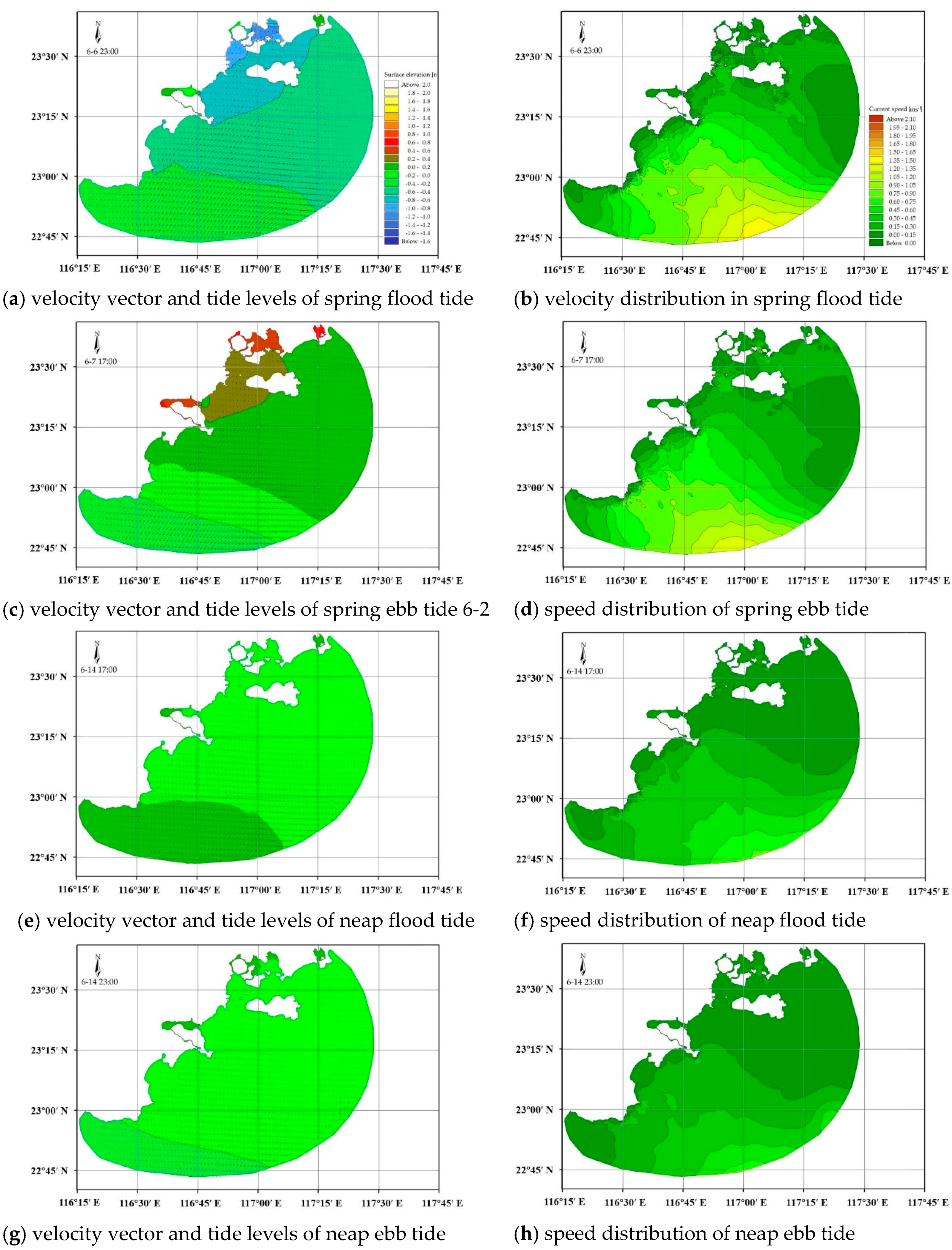
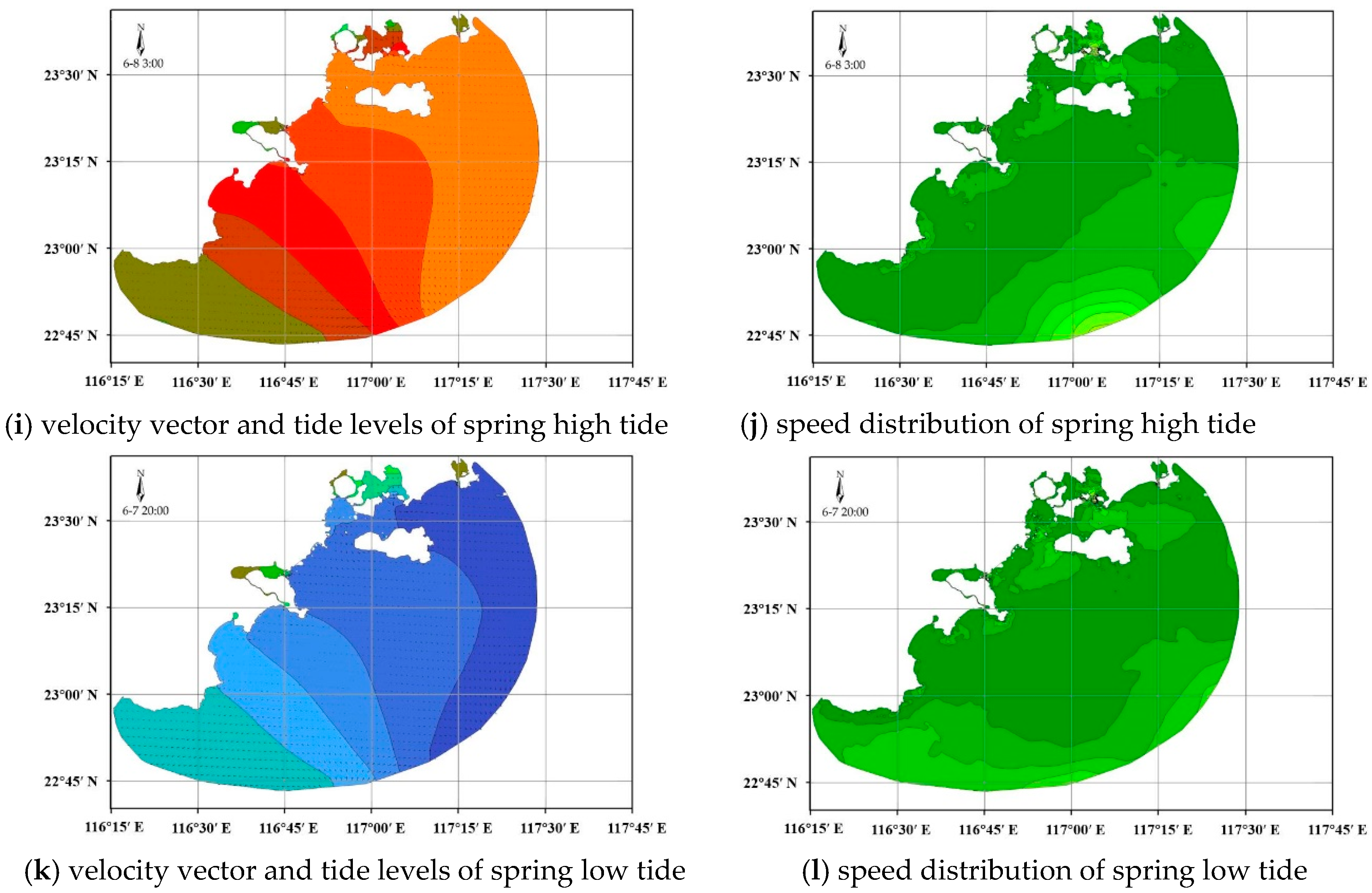
Figure 6 shows the distribution of tide levels and velocity under different conditions. The simulation time includes both astronomical spring tide and neap tide. Selected astronomical spring tide rising time (23:00 on 6 June 2020), astronomical spring tide falling time (17:00 on 7 June 2020), astronomical neap tide rising time (17:00 on 14 June 2020), astronomical neap tide falling time (23:00 on 14 June 2020), high tide flat tide time (3:00 on 8 June 2020), and low tide flat tide time (20:00 on 7 June 2020) are shown in Figure 6.

When there is no strong wind field, the sea water current in the study area is mainly affected by the combined action of tide potential and topography. Rivers also play a significant role in estuaries. The current in the study area is approximately parallel to the coastline. The current is cut-off near the island and split into two currents around it. When the tide is rising, the sea water flows from southwest to northeast. The overall flow direction is roughly parallel to the coastline (see Figure 6a,e). When the tide is falling, the sea water flows from northeast to southwest. It also roughly parallels to the coastline (see Figure 6c,g). The velocity of sea water in the south of the study area is faster than that in the north. Especially in some area near the southern border, the speed during astronomical tides can exceed 1.2 ms⁻¹. However, the sea near Nan’ao Island is relatively calm. The velocity is generally less than 0.5 ms⁻¹ (see Figure 6b,d,f,h,j,l). During high tide, it tends to be high in the northeast and low in the southwest. However, at low tide, it is opposite. The maximum tidal range in the northeast of the study area can be more than 2 m, where this value is less than 1.5 m in the southwest of the study area (compare Figure 6i and Figure 6k). In study area, there are two high tides and two low tides in one lunar day. The amplitude difference between adjacent high tides and low tides is large. The tidal type here is irregular semi-diurnal tides. The flow velocity at flood tide is slightly greater than that at ebb tide. At high tide, the water level in the study area is high in the northeast but low in the southwest. At low tide, it is opposite. The water level difference at high tide is slightly higher than that at low tide in the study area. The tidal range in the northeast of the study area is large, exceeding 2 m, while the tidal range in the southwest is low, less than 2 m. At flat tide, the whole study area is relatively calm. In addition, due to the topography and islands, near the mouth of the river, and in some areas between the island and the land, the water also flows fast.

Figure 6a,b shows the distribution of tide level and current velocity in the study area at astronomical spring tide rising time. At this time, the sea water flows from southwest to northeast, and the overall flow direction is roughly parallel to the coastline. Near the mouth of the Rongjiang River, the bulging terrain of Dahao Island plays a role in blocking the current. Some seawater enters Haojiang River, while others bypass the island. At the east side of Dahao Island, the velocity of the sea water can exceed 1 ms⁻¹ at this time. There are also current diversions on both sides of Nan’ao Island, which are distributed from the east and west sides to bypass the island. This is also a place where the sea flow velocity is high, and the flow velocity can reach 1 ms⁻¹. The tide level in the whole study area showed a trend of high in the southwest and low in the northeast, but the water level is not much different. The water level in the southwest was about 0.4 m higher than that in the northeast. There is a fast flowing area in the south of the study area, while the sea area east of Nan’ao Island is relatively calm. Figure 6c,d shows the distribution of tide level and current velocity in the study area during astronomical spring tide falling time. The water now flows from northeast to southwest, also roughly parallel to the coastline. Compared with the flood tide, the flow velocity near Nan’ao Island is lower at ebb tide, but the flow velocity near Dahao Island is still faster, exceeding 1 ms⁻¹. The sea water flows out of the estuary at ebb tide. At this time, the water level was high in the northeast and low in the southwest. The difference of water level was still small, about 0.4 m. The velocity distribution of sea water in the sea area is roughly the same as that in the spring tide. Figure 6e–h show the distribution of tide level and sea velocity in the study area at astronomical neap flood tide and ebb tides, respectively. At this time, the distribution of tidal current in the study area is basically the same as that at astronomical spring tides. However, the flow velocity is low, generally lower than 0.5 ms⁻¹. The difference in water level in the study area is small. The water level of the whole sea is relatively uniform. Figure 6i,j shows the distribution of tide level and velocity during high tide in the study area. At this time, the current velocity of the whole sea area is slow, and the current velocity of the nearshore part of the whole study area is generally lower than 0.1 ms⁻¹. The tide level of the whole Shantou sea area is high. The water level gradient is large, showing a trend of high in the northeast and low in the southwest, with a difference of more than 1 m. Figure 6k,l shows the distribution of tide level and velocity at low tide in the study area. Consistent with the high tide, the current velocity is slow. On the contrary, the tide level is low in the northeast and high in the southwest, but the water level gradient is slightly smaller than that at the high tide.

Several points are selected to compare the changes in tide level and velocity. Information of these points is shown in

Table 4. Comparison of tide level and tide current at different points.

Region	Location	Offshore Distance	Highest Water Level	Lowest Water Level	Mean Range	Maximum Flow Velocity	Mean Flow Velocity
Chaoyang District	116°39′ E 23°08′ N	50 m	0.839 m	−1.054 m	0.902 m	0.434 ms−1	0.176 ms−1
	116°39′ E 23°09′ N	1500 m	0.841 m	−1.071 m	0.912 m	0.540 ms−1	0.275 ms−1
	116°39′ E 23°07′ N	2500 m	0.842 m	−1.071 m	0.901 m	0.515 ms−1	0.257 ms−1
Haojiang District	116°49′ E 23°14′ N	330 m	1.022 m	−1.374 m	1.282 m	0.602 ms−1	0.333 ms−1
	116°50′ E 23°15′ N	2000 m	1.028 m	−1.351 m	1.270 m	0.594 ms−1	0.314 ms−1
Longhu District	116°49′ E 23°22′ N	170 m	1.113 m	−1.380 m	1.392 m	0.105 ms−1	0.037 ms−1
	116°49′ E 23°21′ N	700 m	1.109 m	−1.379 m	1.389 m	0.106 ms−1	0.045 ms−1
	116°48′ E 23°21′ N	1200 m	1.104 m	−1.379 m	1.385 m	0.147 ms−1	0.064 ms−1
Nan’ao island	117°20′ E 23°30′ N	300 m	1.193 m	−1.599 m	1.569 m	0.582 ms−1	0.261 ms−1
	117°08′ E 23°31′ N	800 m	1.192 m	−1.599 m	1.564 m	0.508 ms−1	0.221 ms−1
	117°08′ E 23°30′ N	1300 m	1.192 m	−1.599 m	1.563 m	0.490 ms−1	0.210 ms−1

.

As shown in Table 4, Chaoyang District is located in the southwest, with the smallest tidal range, which is less than 1 m. Longhu District is blocked by the island. The sea current is most stable with the slowest velocity. It can be seen from Table 4 that the average velocity of Longhu district is less than 0.01 ms⁻¹. Affected by the topography, the velocity and tidal range in Haojiang District and Nan’ao Island are relatively high. As shown in Table 4, the average velocity in Haojiang District and Nan’ao Island is greater than 0.2 ms⁻¹.

The velocity in the nearshore sea area is generally lower than that at the far shore, which is the result of the shallow water depth near the nearshore and sea bottom friction. The speed near the coast is greatly influenced by the terrain. For example, Longhu District is located between Dahao Island and Nan’ao Island. Because of its barrier, the flow velocity is low. In Haojiang District, the water flow is blocked by the island and turns to converge, so the sea water velocity is relatively high. The topographic effect in the vicinity of Nan’ao Island has a significant influence on the tide, resulting in the formation of the current around the island.

3.2. Influence of Different Tidal Constituents

It is generally believed that the South China Sea is mainly affected by the four tidal constituents M2, S2, K1, and O1, which enter from the Luzon Strait. The amplitude of these tidal constituents increases as the water depth becoming shallow [21]. For example, Fang et al. [22] numerically simulated the tidal current distributions of M2, S2, K1, and O1 in the whole South China Sea, including the Beibu Gulf. Wu et al. [23] used the POM model to simulate the tides and tidal currents of M2, S2, K1, and O1 in the South China Sea.

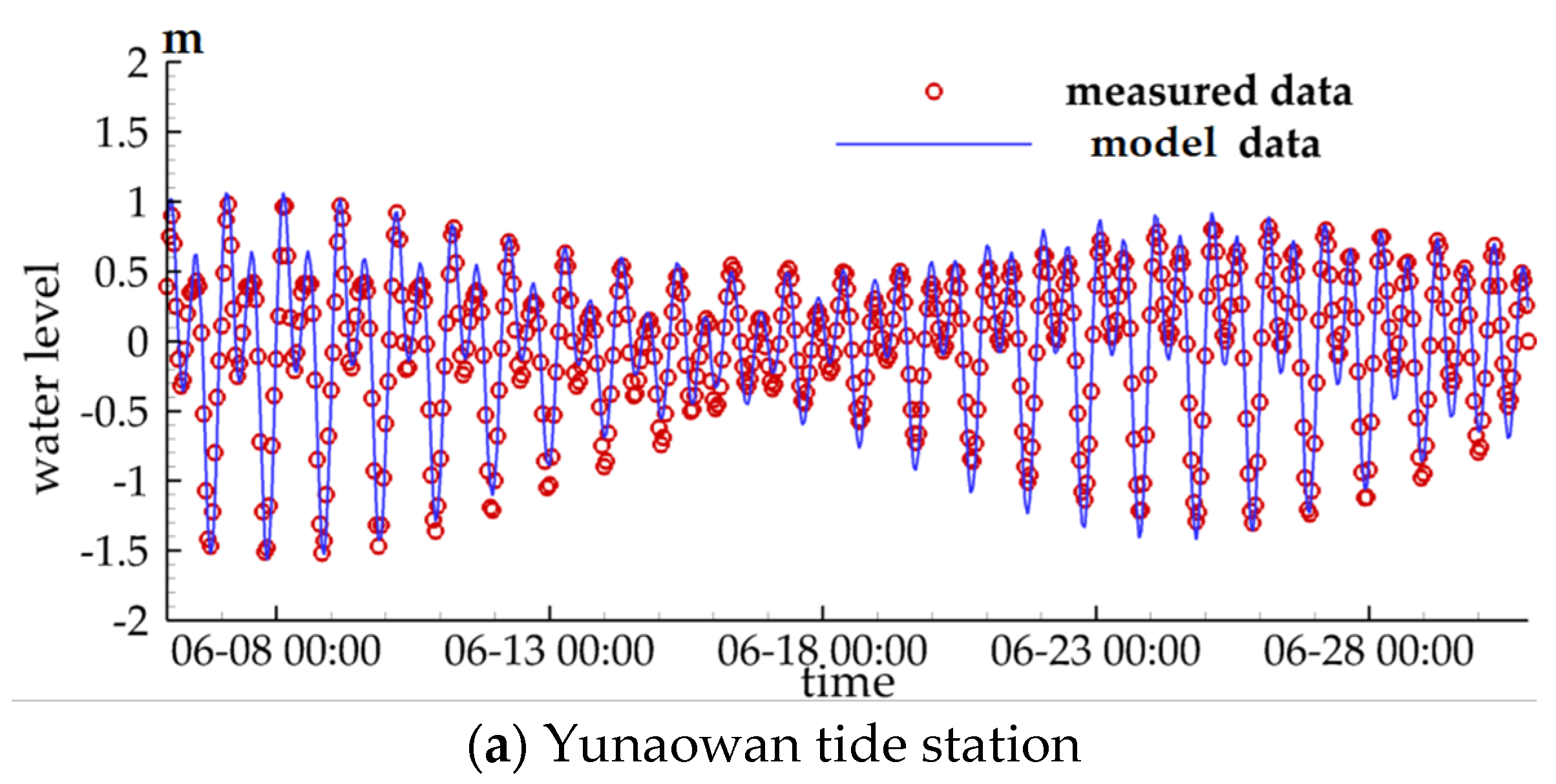
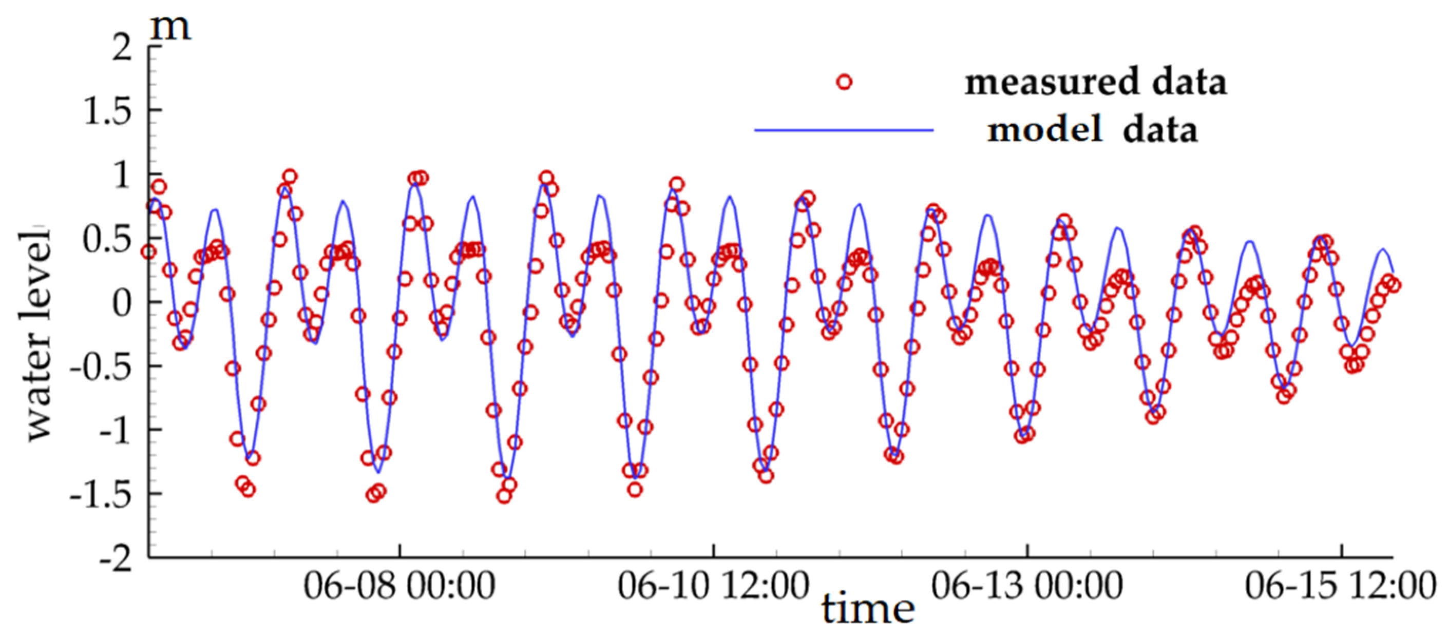
However, in the calibration process of the hydrodynamic model, we found that if only these four tidal constituents are added to the open boundary, the validation effect of the model is not ideal. When only M2, S2, K1, and O1 tidal constituents are considered as tidal potential, taking Yunaowan tide station as an example, the verification results are shown in Figure 7.

Figure 7 shows that when only M2, S2, K1, and O1 tidal constituents are considered, the tide levels in two high tides per day of the model data are basically the same. However, there is a significant difference between the two water levels in the measured tidal data. On this basis, the model added N2, K2, P1, and Q1 tidal constituents successively. The simulation results show that the P1 tidal constituent plays an obvious role in reducing this error. P1 is the solar declination dividual, mainly caused by the tidal potential force of the sun, with a period of 24.066 h. 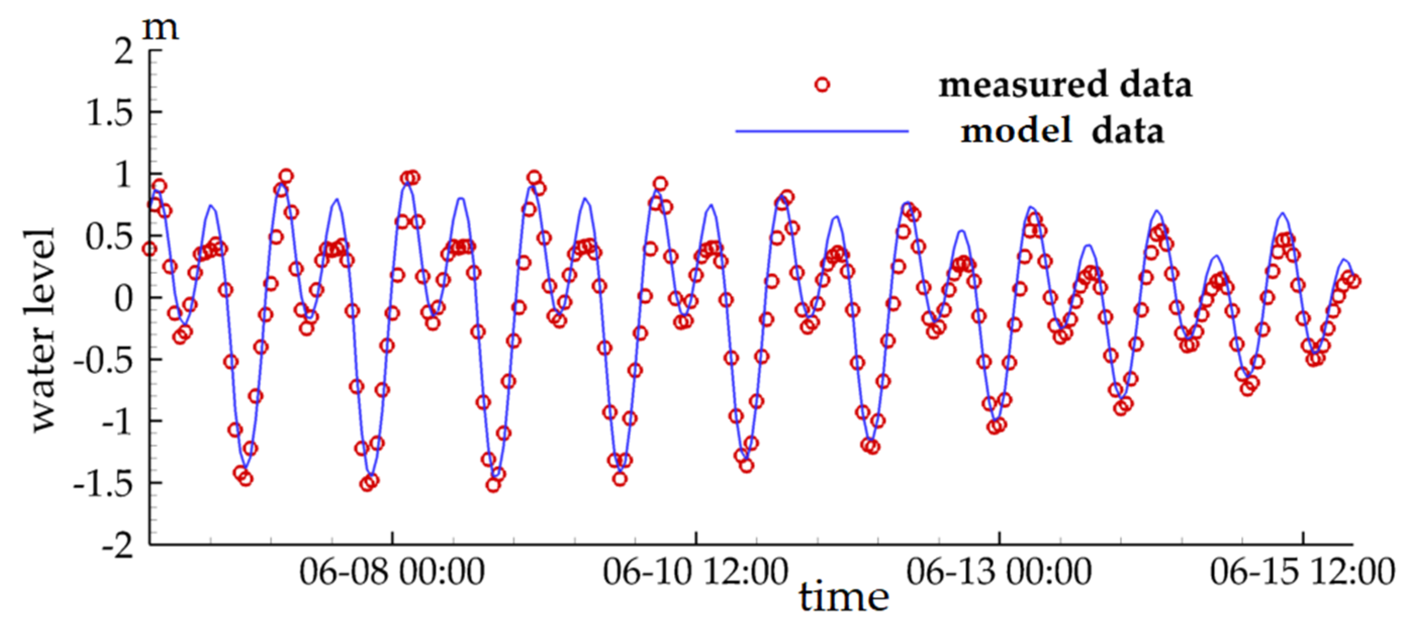Figure 8 takes Yunaowan tide station as an example; it shows the simulation results after adding the P1 tidal constituent to the M2, S2, K1, and O1 tidal components.

Figure 8 shows that the P1 tidal constituent has a great influence on reducing the error above. However, compared with the addition of M2, S2, K1, O1, N2, K2, P1, and Q1 (see Figure 3a), there are still some errors. In the study of the tides in the South China Sea, the four tidal constituents M2, S2, K1, and O1 can basically meet the requirements of accuracy. However, the accuracy of the model will be further improved when more tidal constituents are considered. For example, Lu et al. [24] considered eight tidal constituents M2, S2, K1, O1, N2, K2, P1, and Q1 when studying tidal currents in the northern part of the South China Sea. Tao et al. [25] considered 13 common tidal constituents when studying the Nan’ao Sea Area of Shantou.

Shantou is close to the South China Sea. M2, S2, K1, and O1 tidal constituents basically determine the level and the period of the tide in Shantou. However, there is an error in the lower high tide per day if we only consider these four tidal components. The P1 tidal constituent can effectively reduce this error.

3.3. The Influence of the Typhoon

The typhoon is one of the most destructive weather systems. Storm surges and waves caused by typhoons often bring large damage to coastal areas. On 2 August 1922, a storm surge occurred in Shantou area, with more than 70,000 deaths, which was one of the biggest storm surge disasters of the 20th century [26]. Shantou City often encounters storm surges, mainly typhoons and severe tropical storms every summer [2].

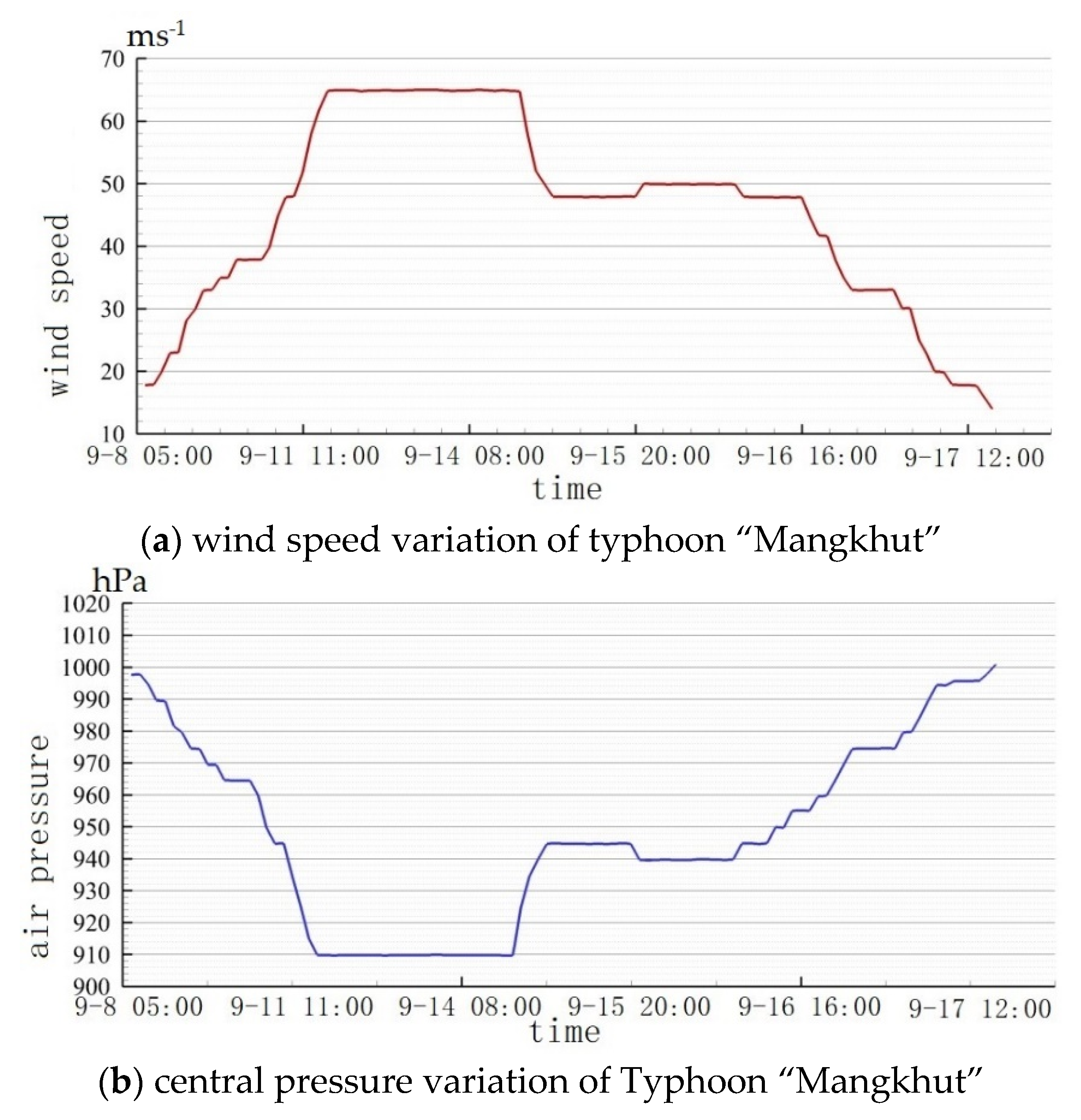
Typhoon “Mangkhut” is a super typhoon that was generated at 20:00 on 7 September 2018 over the Northwest Pacific Ocean. On 10 September, the typhoon moved to the southwest. At 8:00 on 11 September, it became a super typhoon. On 15 September, the typhoon passed through the northern Philippines and moved to Guangdong Province of China. At 17:00 on 16 September, Typhoon “Mangkhut” landed in Haiyan town with a maximum wind force of 14 and a central minimum pressure of 955 hPa. In the afternoon of 17 September, the typhoon weakened to a tropical depression, and then continued to move to the northwest. The typhoon basically dissipated until 20:00 [27]. Figure 9 shows the wind speed and central pressure of Typhoon “Mangkhut”.

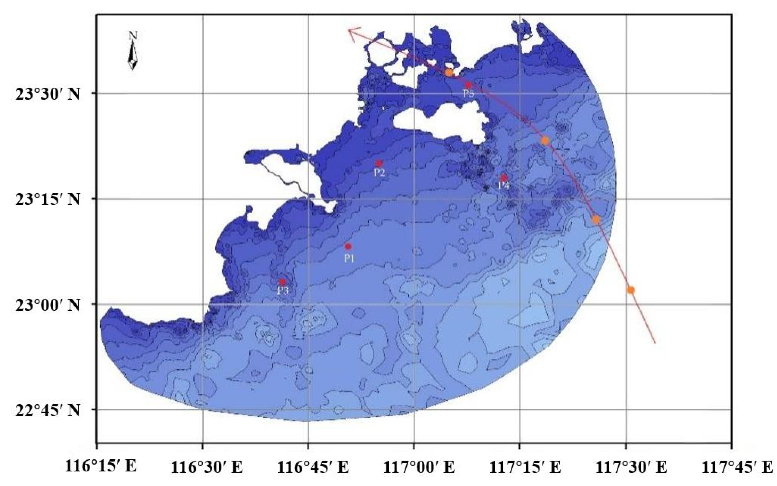
In order to simulate the impact of typhoons on Shantou more truly, the parameters of wind field (including wind speed and central pressure) in the model are the data of Typhoon “Mangokhut”. This is equivalent to moving its route east by 1.2 longitude and north by 1.7 latitude, so that it transits from the northeast side of the study area (see Figure 11). The simulation of the typhoon was conducted by hot start, and the preliminary results were taken as the initial conditions. The simulation lasted for 4 days. 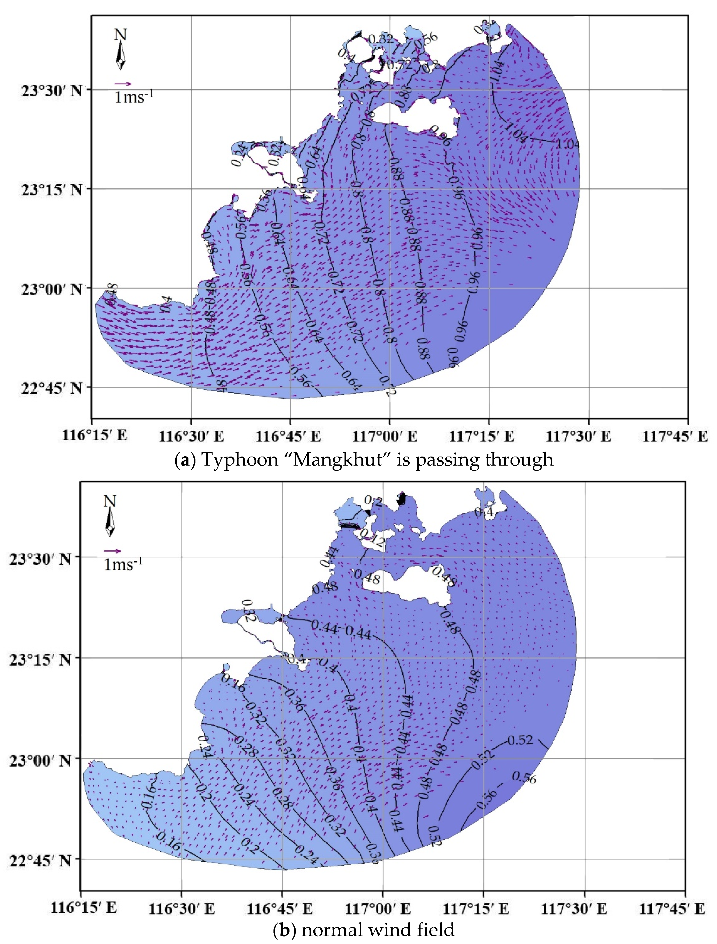Figure 10a shows the distribution of the flow field and water level during the typhoon at the time of high tide. Figure 10b shows the flow field and water level distribution of the normal wind field.

In the presence of the super typhoon, the whole flow field in the study area changed significantly. The water level distribution shows that the closer to the typhoon center, the higher the water level. Compared with normal wind, the water level increased. The water level in the whole sea area increased by more than 0.3 m. Under the influence of the typhoon, the current direction in the study area was the far current pointing to the typhoon center, while the offshore current was similar to the counterclockwise rotation of wind field. The flow velocity also increased greatly, and the main driving force of the flow field in the study area changed from tidal potential to wind field.

The flood disaster caused by a typhoon storm surge is the main way typhoons damage coastal areas. In this model, the path of the typhoon center is located in the northeast of the study area, and the landing place is in the south of Zhao’an County. Taking the typhoon before landing as an example, the calculation shows that when the typhoon passes through, the tide elevation in the south sea area of Zhao’an County increases by 0.32 m. The 0.24 m water level was increased in the sea area to the east of Nan’ao County, and −0.08 m near the Rongjiang River estuary of Dahao Island. The water increased about 0.08 m in the sea area around the Chaoyang area. It can be seen that the closer it is to the typhoon center, the more obvious the increase in water level.

Five typhoon monitoring points were selected to compare the different responses of the water surface height relative to the general state when the typhoon transited, and the different response of speeds when there was no wind, normal wind, and when the typhoon transited. See

Table 5. Information of typhoon monitoring points.

Serial Number	Longitude	Latitude	Bathymetry	Offshore Distance
Point 1	116°52′ E	23°08′ N	31.5 m	12.5 km
Point 2	116°56′ E	23°22′ N	11.5 m	1.8 km
Point 3	116°41′ E	23°06′ N	21 m	7.8 km
Point 4	117°15′ E	23°18′ N	30 m	13.1 km
Point 5	117°04′ E	23°29′ N	4.5 m	0.4 km

and Figure 11 for its distribution and information.

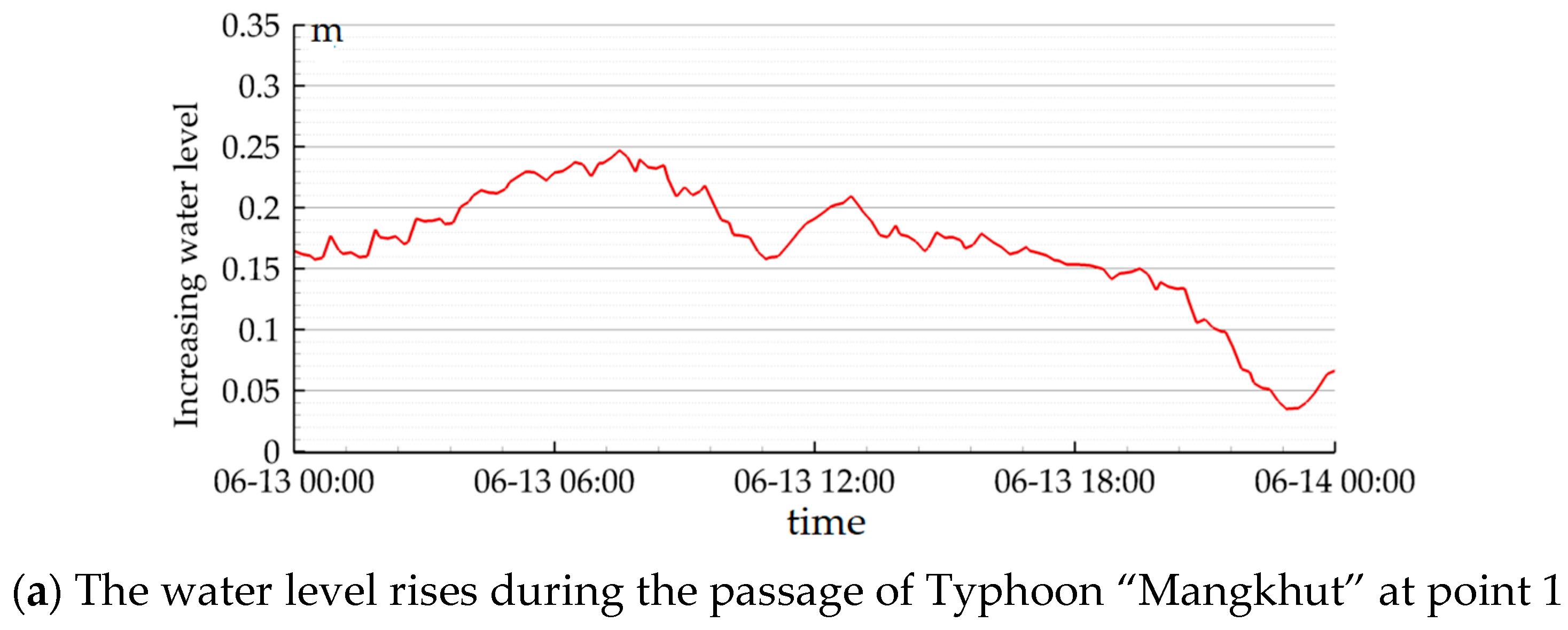
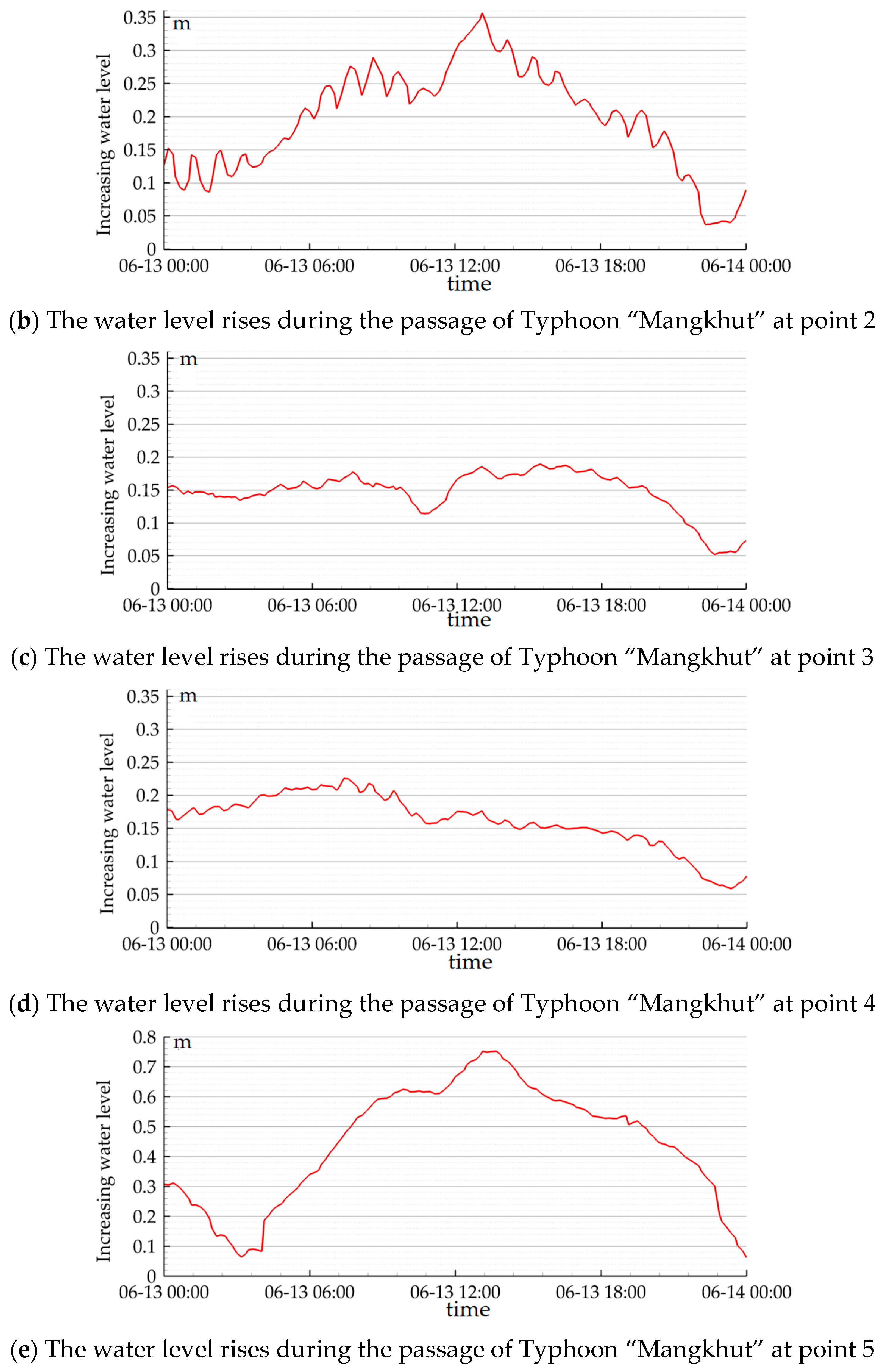
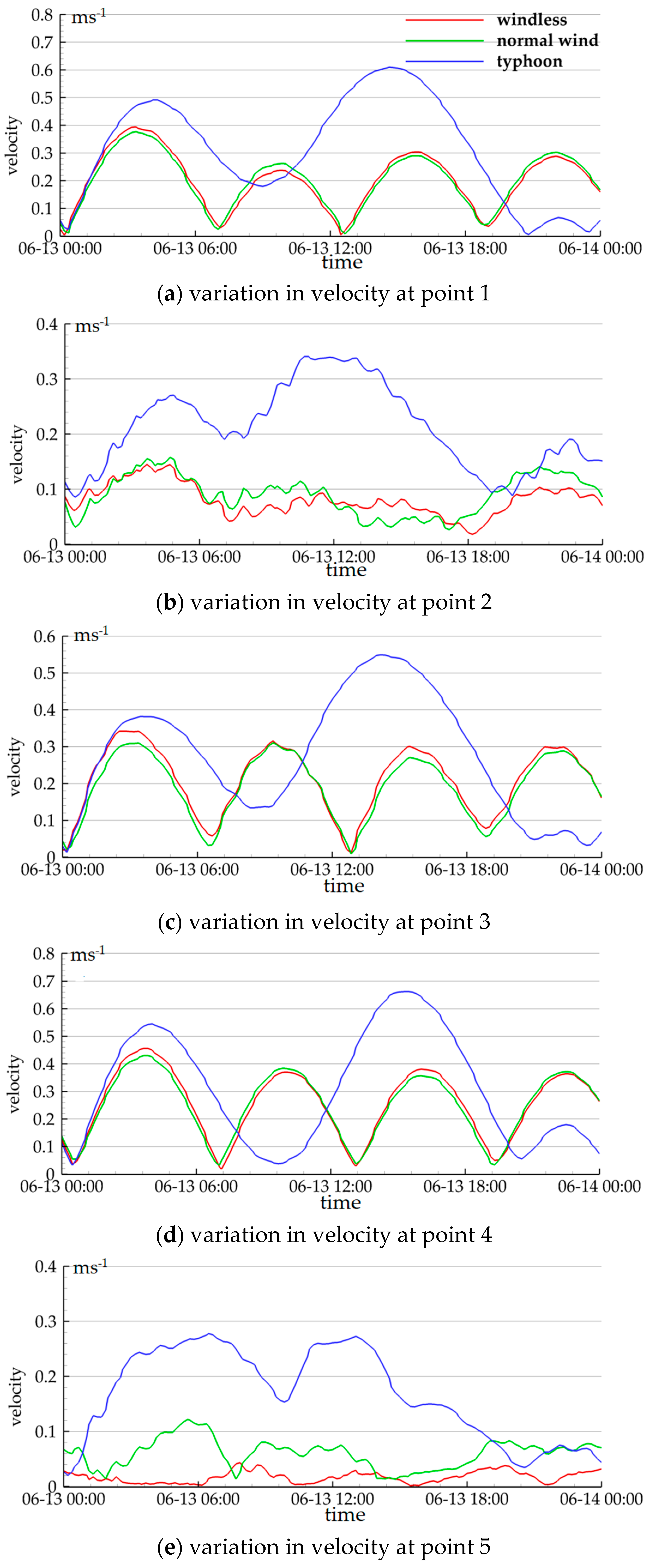
Figure 12 shows the water level when the typhoon was passing through minus the water level of the normal wind field at the same time. Figure 13 compares the sea water velocity in the windless state, the normal wind field, and the typhoon transit.

Figure 12 shows the water level increase comparison of five points. The influence of wind fields is more obvious at the shallow water depth (see Figure 12b,e) than at the deep offshore water depth (see Figure 12a,c,d). When the typhoon passed through, the tide elevation generally increased significantly. Within 24 h, the average water increases at five points were 0.17 m, 0.20 m, 0.15 m, 0.16 m, and 0.45 m, respectively. The maximum water increases were 0.24 m, 0.35 m, 0.19 m, 0.23 m, and 0.75 m, respectively. In addition to the tide level, the typhoon also affects the velocity of the sea. In Figure 13, the red line means there is no wind in the area. The green line is the normal wind field and the blue line is the wind field of typhoon “Mangkhut”. Figure 13 shows the variation in velocity under different wind conditions. In the region of high current velocity, the sea current velocity is mainly controlled by tide, and the influence of the normal wind field is limited (see Figure 13a,c,d). In the area of low current velocity, the sea current velocity is less affected by the tide. The normal wind can also cause a larger change in the velocity (see Figure 13 b,e). When a typhoon exists, the sea current velocity is mainly determined by the typhoon at any control point (see Figure 13a–e).

The nearshore water depth is shallow, where the storm surge caused by the typhoon increases in wave height, the energy converges, and the water level overlaps online-early, showing a large-scale increase in water. Therefore, it is very necessary to protect the coast during the passage of the typhoon. In the presence of a typhoon, the speed can be increased by several times, so the influence of wind field should be especially considered when a typhoon is operated offshore. In areas far from the coast, the wind field changes the velocity equally dramatically. In the case of normal wind field, the flow velocity is still mainly controlled by the tide potential. In the case of a typhoon, the distribution of the flow velocity is completely different, which indicates that the wind dominates the flow field at this time. At the same time, it should be noted that in the case of the typhoon, the flow direction of sea current is also mainly controlled by the wind field (Figure 10). When there is no typhoon, there are four maximum values of sea water velocity in the study area in a day, while there are only two maximum values when the typhoon comes. The tide in the Shantou sea area is an irregular semidiurnal tide; there are two high tides and two low tides in a day, so there are four maxima of velocity in one day. When the typhoon comes, sea water flow is mainly controlled by the typhoon. When the sea current caused by the tide is in the same direction as the sea current caused by the typhoon, the flow velocity will overlap and increase in speed. However, when the current direction caused by the tide is opposite to that caused by the typhoon, the two offset each other, making the velocity lower than that without the typhoon. Therefore, when a typhoon passes through, the sea surface can only have two maximum velocity values in one day.

Typhoon “Mangkhut” is a case of many typhoons, belonging to the intensity and harm of the greater typhoon. However, in most cases, the typhoon landing in Shantou was not a super typhoon. In order to better reflect the change in sea surface flow field and the increase in water level caused by typhoon storm surges of different levels, four typhoon scenes with different recurrence periods were defined. The central pressure of a typhoon was given by a hurricane model and the typhoon parameters were determined to correspond to the model to reconstruct the wind field.

The most important parameters that determine the scale of the typhoon wind field are the minimum pressure of the typhoon center (P0), the radius of maximum wind speed (R_max), the maximum wind speed (V_max), and the moving path of the typhoon. Among them, the maximum wind radius of the typhoon can be estimated according to the empirical formula [29,30], and its maximum wind radius is related to the minimum pressure of the typhoon center:

$$R_{\max }=1119.0\times (1010-P_0{)}^{-0.806}$$

(8)

The maximum wind speed of the typhoon can also be calculated according to the empirical formula [31], which is expressed as follows:

$$V_{\max }=3.7237\times {(1010-P_0)}^{0.6065}$$

(9)

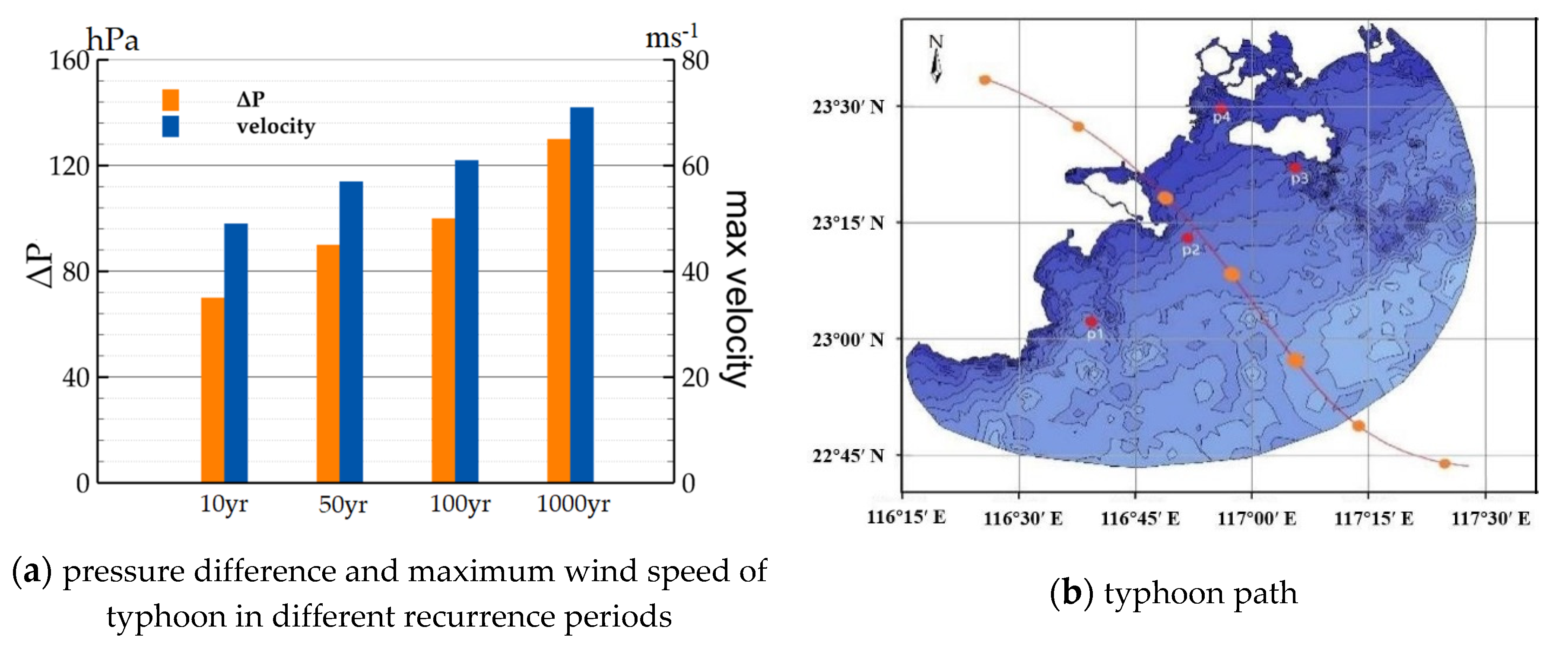
In this study, four typhoons with different central pressures were constructed, and each typhoon represented a different recurrence period. The four typhoons have the same path and all landed in Shantou. The typhoon path is shown in Figure 14. The information of each typhoon is shown in

Table 6. Information of each typhoon.

Number	Central Pressure	Maximum Wind Speed	Maximum Wind Radius	Recurrence Period
1	940 hPa	49 ms−1	36 km	10 yr
2	920 hPa	57 ms−1	30 km	50 yr
3	910 hPa	61 ms−1	27 km	100 yr
4	880 hPa	71 ms−1	22 km	1000 yr

:

As shown in Figure 14, the typhoons enter the sea area of Shantou City from the outside sea and land near the mouth of Rongjiang River. They pass through the main urban area of Shantou. Typhoons land at the time of astronomical spring tide, so the increase in water level caused by the typhoon and the increase in water level caused by the tide are superimposed. The simulation time of each typhoon is 72 h. 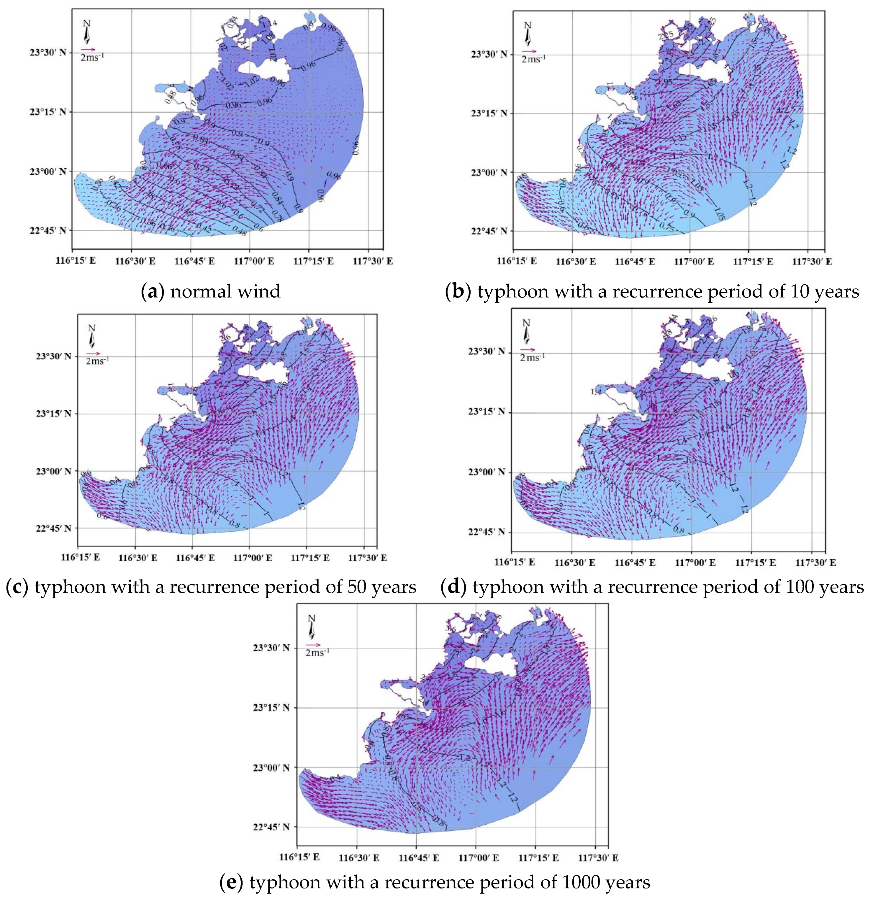Figure 15 shows the distribution of isobathymetric lines and the change in flow field in the Shantou sea area during the passage of typhoons with different intensities.

Figure 15a shows the comparison when there is no typhoon. This moment is the high tide of the astronomical spring tide. The sea water flows from northeast to southwest. Figure 15b–e, respectively, show the situation of typhoons with recurrence periods of 10 years, 50 years, 100 years, and 1000 years. The central air pressure of the typhoon is set at 940 hPa, 920 hPa, 910 hPa, and 880 hPa, respectively. When a typhoon appears, the sea current in the study area is controlled by the typhoon. In the model, the typhoon center path roughly passes through the center of the study area, moves from southeast to northwest, and lands in Shantou City near the Rongjiang River estuary. The northeast side of the Rongjiang River estuary is on the right side of the typhoon path, while the southwest side of the Rongjiang River estuary is on the left side of the typhoon path. Shantou City is located near the Tropic of Cancer, belonging to the northern hemisphere, affected by the geotropic deflection force. The typhoon wind field has counterclockwise rotation. In the study area, the water flow on the northeast side basically flows from south to north, while on the southwest side, the velocity vector is roughly the same as that of the typhoon, indicating that the direction of the water flow was controlled by the typhoon at this time. The flow direction of sea water is basically the same under typhoons of different intensities. In terms of velocity, the sea current is affected by both the wind field and the tide. On the left side of the typhoon path, the wind is in the same direction as the current caused by the tide. The superposition of the two makes the flow rate fast. On the right side of the typhoon path, the direction of wind is opposite to the direction of the tide. The velocity of the two is offset, so the velocity is not as fast as the sea water on the right side of the typhoon path. By comparing the distribution of sea level in the absence of typhoons, it can be found that the presence of typhoons will obviously cause a rise in sea level and a decrease in water level gradient. The more intense the typhoons are, the more the water level is increased.

Four control points were selected, two on the right side of typhoon path and two on the left side of the typhoon path. Control points were used to compare the height and velocity of the water increase caused by the typhoon in different recurrence periods (see Figure 14). The information of control points is shown in

Table 7. Location, bathymetry, and offshore distance of 4 control points.

Serial Number	Longitude	Latitude	Bathymetry	Offshore Distance
Point 1	116°36′ E	23°06′ N	21.2 m	2.4 km
Point 2	116°50′ E	23°14′ N	13.1 m	3.2 km
Point 3	117°04′ E	23°23′ N	16.4 m	3.8 km
Point 4	116°56′ E	23°30′ N	6 m	1.8 km

. Point 1 and point 2 are located on the left side of the typhoon path. Point 3 and point 4 are located on the right side of the typhoon path.

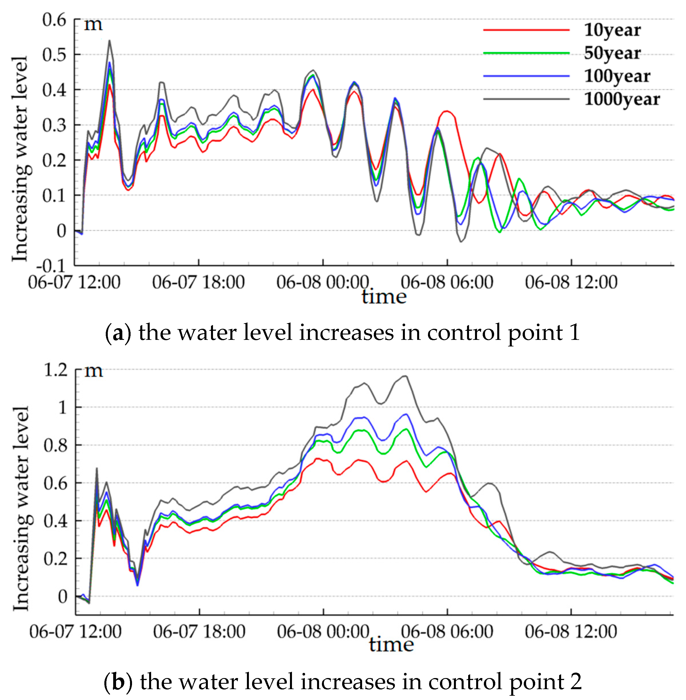
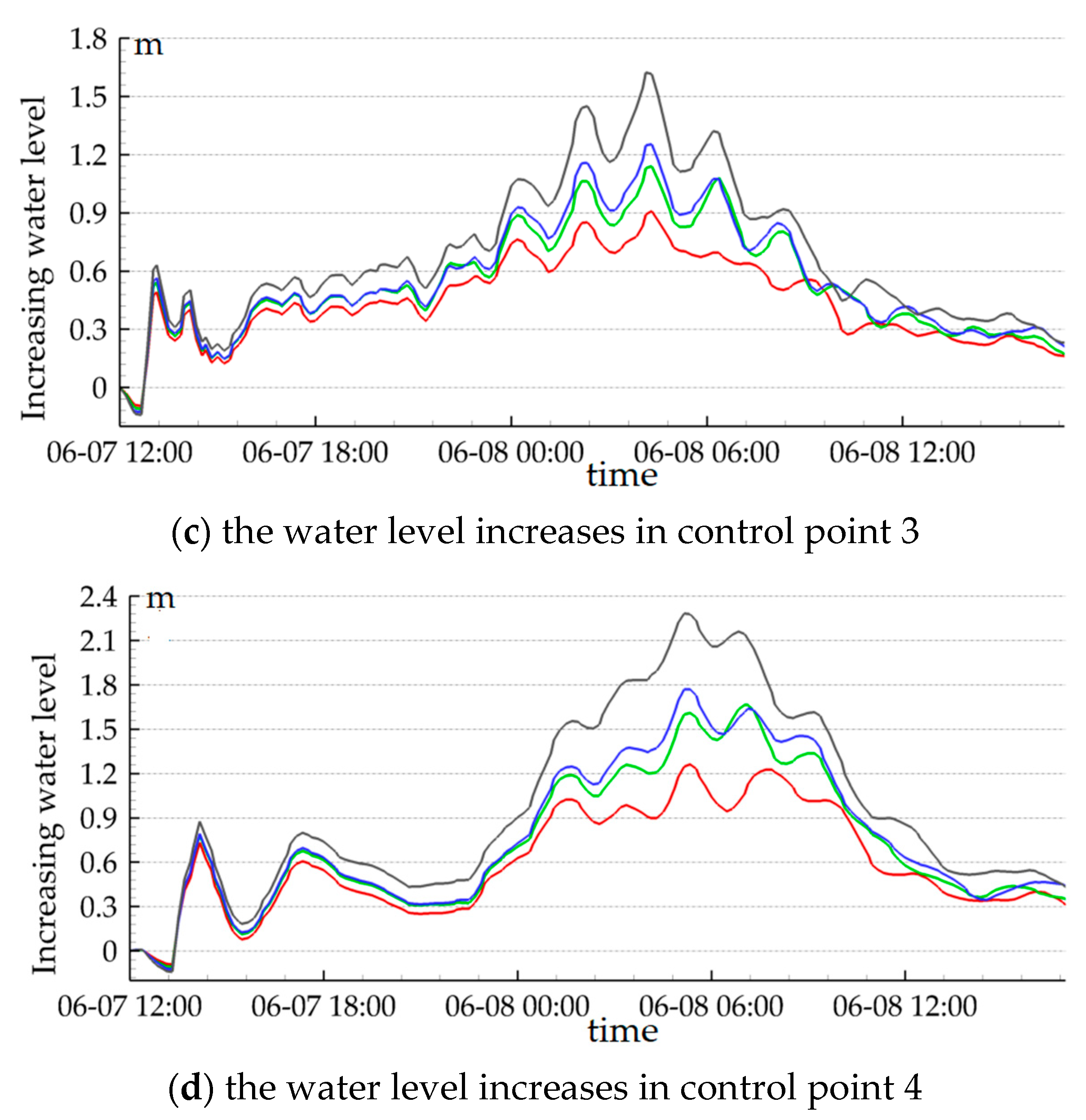
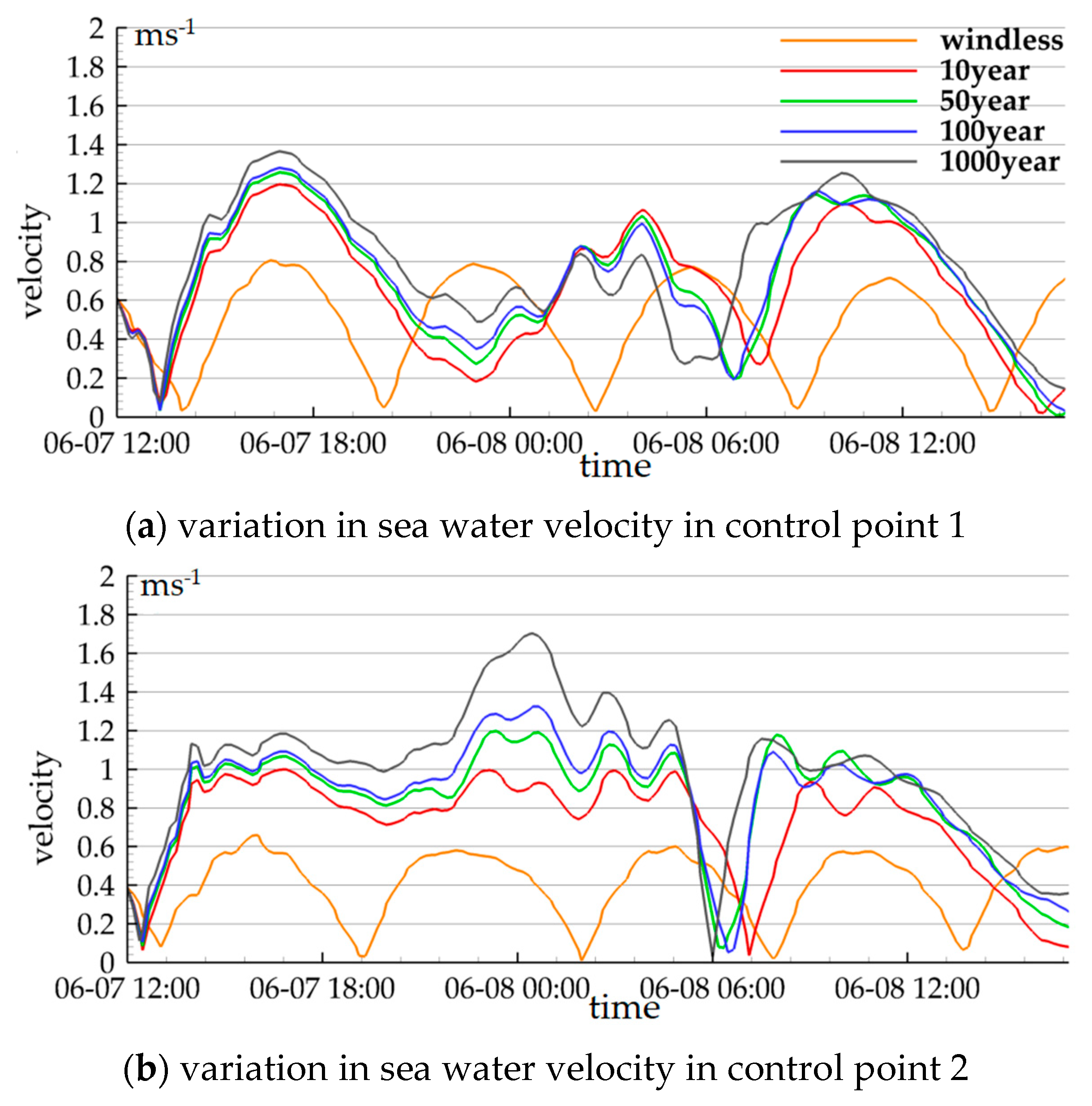
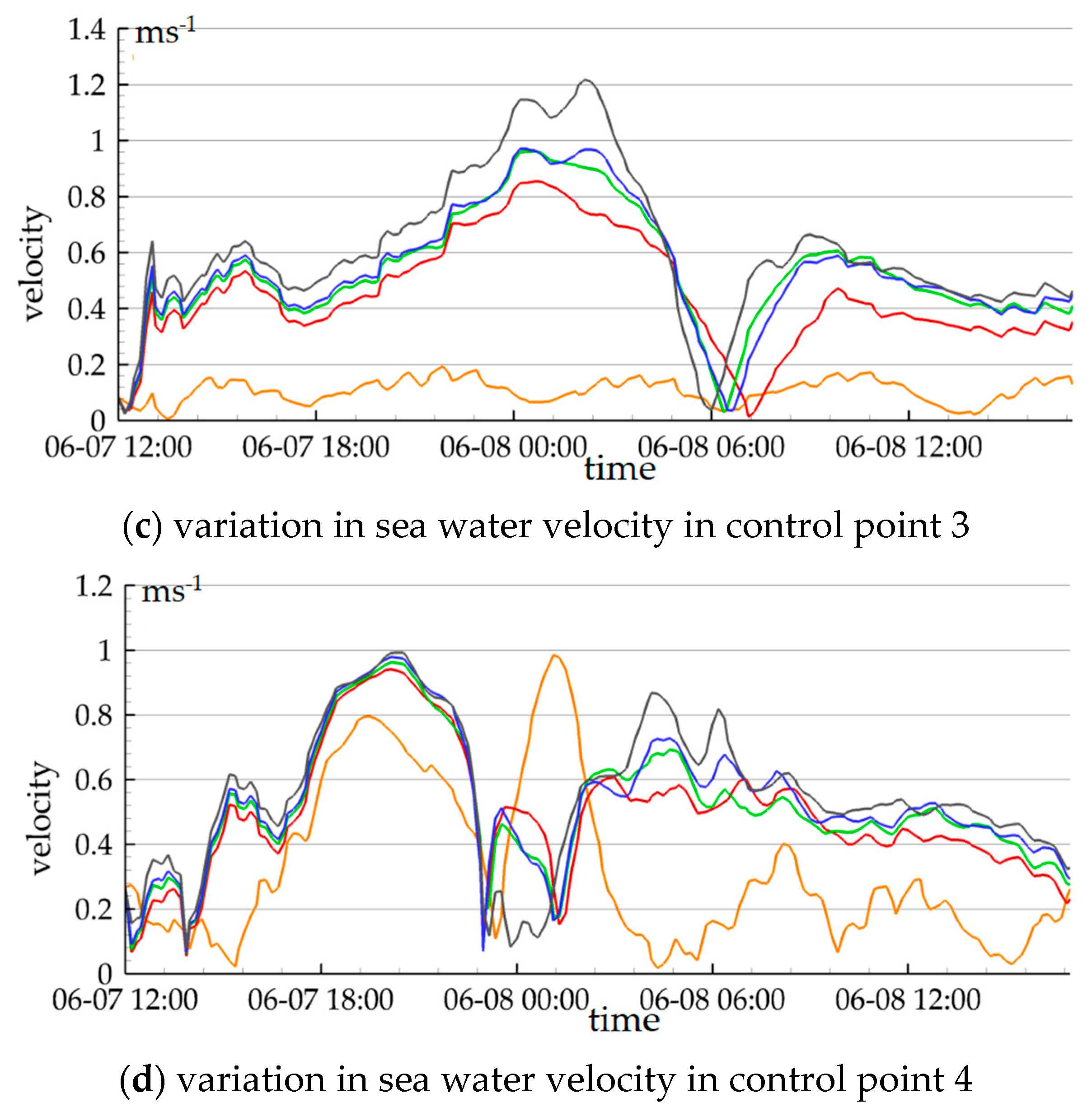
Figure 16 shows the increment in water level in the typhoon with different recurrence periods compared with the normal wind field. Figure 16a–d, respectively, correspond to the four control points selected. Figure 17 shows the changes in sea water velocity in the passage of typhoons in different recurrence periods and compares them with those in the absence of typhoons. Figure 17a–d, respectively, correspond to the four control points selected.

In Figure 16a,b, the water increase at these two points is relatively small. In particular, at point 1 in Figure 16a, the water increase does not exceed 0.6 m. There is just a little difference in the water level increase caused by typhoons of different intensities. In Figure 16b, only typhoons with a recurrence period of 1000 years can increase the water by more than 1 m. However, the impact of typhoons with different intensities is quite different. The increase in water in the millennium-scale typhoons is twice that in the decade-scale typhoons. In Figure 16c,d, points 3 and 4 are located on the right side of the typhoon path. The typhoon-induced water increases are intense at these two control points. In particular, in Figure 16d, even a typhoon with a 10-year recurrence period can cause an increase of more than 1.2 m. The amplitude of the water increase caused by typhoons in different recurrence periods is different, but the process of water increase is roughly the same. As can be seen in Figure 17, the increase in sea water velocity caused by typhoons is shown. The stronger the typhoon, the greater the maximum velocity of sea water. However, the increase in velocity is not as obvious as the water level. In contrast to the increase in water, the velocity of sea water at points 1 and 2 is greater than that at points 3 and 4.

It can be seen from the curve that the rise in water level in the whole sea area caused by the typhoon is oscillating. Point 1 is located on the left side of the typhoon path and on the southwest of the whole sea area. When there is no typhoon passing through, the tidal current is relatively simple and the water level is low. The intensity of increasing water caused by the typhoon is weak here. Even the water increase caused by a typhoon with a recurrence period of 1000 years is less than 0.7 m. The wind vector of a typhoon does not point to the coast here, so the water level increase caused by the typhoon is relatively small. Point 2 is located near the Rongjiang River estuary; it is very close to the typhoon center path. When the typhoon enters the study area, the effect of increasing water is obvious, but the range of increasing water decreases rapidly afterward. As the typhoon gets closer, the wind increases, and the water level begins to rise continuously. After that, the typhoon lands and gradually drifts away, and the rising water level begins to decline slowly. Point 3 is located on the south side of Nan’ao Island, on the upper right of the typhoon path. Its water increase curve is basically the same as that at Point 2. However, the wind vector of the typhoon points roughly to the coast here, which makes the sea water converge toward the coast. The water increasing effect of the storm surge is more obvious. Typhoons with a 50 year recurrence period can lead to a water increase of more than 1 m. The water level drops slowly here, and the water increase duration of the storm surge is long. Point 4 is located in the narrow sea area between the northwest side of Nan’ao Island and the land. The tidal range here is large with normal wind. When a typhoon passes through, it is affected by the wind field and blocked by the terrain, and a large amount of seawater overflows and gathers, resulting in a significant increase in the water level. Even a typhoon in the 10 year recurrence period caused the water level to rise by more than 1 m. The increase in water here is large and lasts for a long time. The large increase in water here will easily cause seawater to enter the land, causing serious harm. It is the key area for typhoon disasters prevention. When a typhoon is passing though, the velocity of each control point will be controlled by the wind field and tide at the same time. Taking Figure 17a as an example, the wind vector and tide current are in the same direction at about 18:00 on 7 June. The velocity of the water at this time was accelerated. The typhoon vector and tide current directions are opposite at about 23:00 on 7 June. This causes the velocity of the water to decrease instead. It is worth noting that the increase in water caused by the typhoon is not completely consistent with the change in velocity. For example, at point 4, the water increase range is highest, but the sea water velocity is not highest, which is less than 1 ms⁻¹.

In this section, we simulated the typhoon “Mangkhut” and four typhoons with different intensities. Typhoon “Mangkhut” belongs to the type of landfall from the east and the rest of the typhoons landed from the front. When Typhoon “Mankhut” landed, its central pressure was close to 910 hPa. Its intensity approached that of a typhoon with a recurrence period of 100 years. However, compared with typhoons with a recurrence period of 50 years, the water increase caused by Typhoon “Mangkhut” was small. This is a better indication that the damage was worse on the right side of the typhoon’s path. About 35% of the typhoons in Shantou belong to the easterly landing type. The increase in water brought by this kind of typhoon is smaller than that landing from the west and front. If the typhoons landing from the east are weak, simple countermeasures can be enough, such as stopping marine activities. Of course, when the typhoon intensity is large, it may still lead to a great water increase, especially in the northeast coast of Shantou city. The four typhoons constructed in the model are all landing from front. They all bring great storm surge disasters. Especially in the northeast coast of Shantou city, such as Chenghai District and Nan’ao Island, the storm surge disaster is huge. The tidal range in Shantou city is larger in the northeast than in the southeast. The key areas for storm surge prevention are the coastal areas in the northeast of Shantou and Nan’ao Island. Once-in-a-century typhoons are relatively rare, so our advice is focused on the more common typhoons. For the northeast coast of Shantou with a large tidal range and easily affected by storm surge, it is suggested to build high dikes to cope with the disaster. More adequate contingency plans, such as evacuation routes and shelters, should be made for these areas. The southeast of Shantou city has a small tidal range and is located on the left side of the path of the typhoons landing front, so the storm surge disaster is relatively small. However, it is necessary to make emergency plans well.

4. Conclusions

The main conclusions of this paper are as follows:

(1) The direction of tidal current in Shantou coastal area is basically parallel to the shore-line. It flows from southwest to northeast at high tide and the flow direction is opposite at low tide. The water level is high in the northeast and low in the southwest at high tide, but it is opposite at low tide.

(2) Due to the many islands in the northeast area of the Rongjiang River estuary boundary, the flow field is complex, the velocity is fast, and the tidal range is large. The number of islands in the southwest part is small, the flow field is relatively simple, and the tidal range is small.

(3) Tides in the study area are mainly controlled by four component tides: M2, S2, K1, and O1, but there is an error in the lower high tide per day if we only consider these four tidal components. The P1 tidal constituent can effectively reduce this error.

(4) In general, the main driving force of the sea current in the study area is the tidal potential. When the typhoon passes through, the wind field also disturbs the current. The typhoon will cause a change in the flow field, so the distant sea water flows to the typhoon center. The sea water around the typhoon will rotate and the velocity will increase, bringing about an abnormal water increase.

(5) When the typhoon directly attacks Shantou, the northeast side of the study area is greatly affected by the typhoon, and there is an obvious water increase, while the southwest side has a slightly small impact, and the water increase range is slightly low. Therefore, the northwest coastal areas of Nan’ao Island need to pay more attention to storm surge disaster prevention.

References

1. Zhao, E.J.; Sun, J.K.; Tang, Y.Z.; Mu, L.; Jiang, H.Y. Numerical investigation of tsunami wave impacts on different coastal bridge decks using immersed boundary method. Ocean Eng. 2020, 201, 107132. [Google Scholar] [CrossRef]
2. Cai, W.T. Characteristics of storm surge along Shantou coast. Public Commun. Sci. Technol. 2013, 5, 111–113. [Google Scholar]
3. Liu, J. A High Resolution Numerical Forecast Model for Storm Surge Floodplain in Shantou Area. Master’s Thesis, Ocean University of China, Qingdao, Shandong, China, 2004. [Google Scholar]
4. Chan, J.C.L.; Shi, J.E.; Liu, K.S. Improvements in the seasonal forecasting of tropical cyclone activity over the western North Pacific. Wea Forecast. 1998, 13, 997–1004. [Google Scholar] [CrossRef]
5. Zhao, E.J.; Qu, K.; Mu, L. Numerical study of morphological response of the sandy bed after tsunami-like wave overtopping an impermeable seawall. Ocean Eng. 2019, 186, 106076. [Google Scholar] [CrossRef]
6. Zhou, B. An overview of the discretization methods of governing equations in computational fluid dynamics. Technol. Econ. Guide 2017, 21, 146. [Google Scholar]
7. Zhao, E.J.; Dong, Y.K.; Tang, Y.Z.; Xia, X.Y. Performance of Submerged Semi-circular Breakwater Under Solitary Wave in Consideration of Porous Media. Ocean Eng. 2021, 223, 108573. [Google Scholar] [CrossRef]
8. Lai, W.F.; Pan, J.Y.; Adam, T.D. Impact of tides and winds on estuarine circulation in the Pearl River Estuary. Cont. Shelf Res. 2018, 168, 68–82. [Google Scholar] [CrossRef]
9. Liu, R.Z.; Zhu, Q.Y.; Ni, P.T. Numerical simulation of storm surge in the Pearl River estuary area. Guangdong Water Resour. Hydropower 2018, 4, 6–10. [Google Scholar]
10. Xu, R.G.; Wang, S.C.; Xie, M.X. Research on the hydrodynamic and silt backsilting in western Shenzhen Port area. Port Eng. Technol. 2020, 31, 81–90. [Google Scholar]
11. Jia, R.P.; Dou, M.; Mi, Q.S. MIKE21 based 2d water environment numerical simulation of Marlboro Lake. Environ. Pollut. Control. 2018, 40, 527–532. [Google Scholar]
12. Xu, T. Overview and application examples of Danish MIKE21 model. Water Conserv. Sci. Technol. Econ. 2010, 16, 867–869. [Google Scholar]
13. Zheng, P.N.; Song, J.; Zhang, F.N. Introduction to common numerical models of the ocean. Mar. Forecast. 2008, 4, 108–120. [Google Scholar]
14. Chen, T.Q.; Zhang, Q.H.; Wu, Y.S. Development of a wave-current model through coupling of FVCOM and SWAN. Ocean Eng. 2018, 164, 443–454. [Google Scholar] [CrossRef]
15. Zhao, E.J.; Dong, Y.K.; Tang, Y.Z.; Sun, J.K. Numerical Investigation of Hydrodynamics and Local Scour around Submarine Pipeline under Joint Effect of Solitary Wave and Current. Ocean Eng. 2021, 222, 108553. [Google Scholar] [CrossRef]
16. Zhou, J.; Zeng, C.; Wang, L.L. The influence of drag coefficient of wind stress on numerical simulation of wind flow. J. Hydrodyn. 2009, 24, 440–441. [Google Scholar]
17. Wu, J. The sea surface is aerodynamically rough even under light winds. Bound. Layer Meteorol. 1994, 69, 149–158. [Google Scholar] [CrossRef]
18. Le, F. A new dynamic formula for determining the coefficient of Smagorinsky model. Theor. Appl. Mech. Lett. 2011, 1, 032002. [Google Scholar]
19. Chen, C.S.; Beardsley, R.C.; Cowles, G. An unstructured grid, finite-volume coastal ocean model (FVCOM) system. Special issue entitled “Advance in computational oceanography”. Oceanography 2006, 19, 78–89. [Google Scholar] [CrossRef] [Green Version]
20. Zhao, C.; Lv, X.G.; Qiao, F.L. Numerical study of tidal wave in Beibu Gulf. Acta Oceanol. Sin. 2010, 32, 1–11. [Google Scholar]
21. Wang, D.S.; Liu, X.D.; Zhuang, H.D. Three-dimensional tidal simulation and tidal flow numerical simulation in the Taiwan Strait based on FVCOM. Mar. Sci. 2016, 37, 10–19. [Google Scholar]
22. Fang, G.Y.; Kwok, K.; Zhu, Y. Numerical simulation of principal tidal constituents in the South China Sea, Gulf of Tonkin and Gulf of Thailand. Cont. Shelf Res. 1999, 19, 845–869. [Google Scholar] [CrossRef]
23. Wu, Z.; Tian, Z.W.; Zhao, Q. Three-dimensional tidal wave assimilation numerical simulation in the South China Sea. J. Hydrodyn. 2004, 19, 501–506. [Google Scholar]
24. Lu, M.; Ding, Y.; Si, M.C. Typhoon response in the northern part of the South China Sea. Trans. Oceanol. Limnol. 2019, 5, 9–19. [Google Scholar]
25. Tao, Y.J.; Zhang, L.; He, Q.Q. Numerical analysis of the hydrodynamic force of typical typhoons in Nan’ao area of Shantou. Pearl River 2019, 40, 48–55. [Google Scholar]
26. Hong, Y.J.; Lin, Y.S.; Chen, W.Z. China’s worst typhoon of the century caused a tidal disaster. J. Catastrophol. 1986, 1, 62–63. [Google Scholar]
27. He, Y.C.; He, J.Y.; Chen, W.C.; Chan, P.W. Insights from Super Typhoon Mangkhut (1822) for wind engineering practices. J. Wind Eng. Ind. Aerodyn. 2020, 203, 104238. [Google Scholar] [CrossRef]
28. Liu, Z.K.; Li, J.G.; Li, H. Analysis and suggestion of wave damage caused by Typhoon Manchu on the South China Sea platform. Shipbuild. China 2019, 60, 197–203. [Google Scholar]
29. Vickery, P.J.; Skerlj, P.F.; Twisdale, L.A. Simulation of hurricane risk in the US using empirical track model. J. Struct. Eng. 2000, 126, 1222–1237. [Google Scholar] [CrossRef]
30. Cheung, K.F.; Tang, L.; Donnelly, J.P.; Scileppi, E.M.; Liu, K.B.; Mao, X.Z.; Houston, S.H.; Murnane, R.J. Numerical modeling and field evidence of coastal overwash in southern New England from Hurricane Bob and implications for paleotempestology. J. Geophys. Res. Earth Surface 2007, 112, F3. [Google Scholar] [CrossRef] [Green Version]
31. Atkinson, G.D.; Holliday, C.R. Tropical cyclone minimum sea level pressure maximum sustained wind relationship for the western North Pacific. Mon. Weather Rev. 1977, 105, 421–427. [Google Scholar] [CrossRef] [Green Version]
Figure 1. Study area and oceanographic station location. (The blue squares are the tide stations; the red circles are the ADCP points).
Jmse 09 00912 g001
Figure 2. Grid division diagram of the study area.
Jmse 09 00912 g002
Figure 3. Verification results of tide level.
Jmse 09 00912 g003aJmse 09 00912 g003b
Figure 4. Velocity validation.
Jmse 09 00912 g004
Figure 5. Direction verification.
Jmse 09 00912 g005aJmse 09 00912 g005b
Figure 6. Distribution of tide levels and current speed in the study area.
Jmse 09 00912 g006aJmse 09 00912 g006b
Figure 7. Tidal constituent verification for M2, S2, K1, and O1.
Jmse 09 00912 g007
Figure 8. Tidal constituent verification for M2, S2, K1, O1, and P1.
Jmse 09 00912 g008
Figure 9. Wind speed and air pressure in the center of Typhoon “Mangkhut” (data of Typhoon “Mangkhut” according to Liu [28]).
Jmse 09 00912 g009
Figure 10. Water level line and flow field map of typhoon transit compared with normal wind field conditions.
Jmse 09 00912 g010
Figure 11. Path of typhoon “Mangkhut” in model and location of typhoon monitoring points.
Jmse 09 00912 g011
Figure 12. The increment in water level during the passage of Typhoon “Mangkhut”.
Jmse 09 00912 g012aJmse 09 00912 g012b
Figure 13. Variation in velocity under different wind conditions.
Jmse 09 00912 g013
Figure 14. Typhoon intensity and its path (red circles are the selected control points).
Jmse 09 00912 g014
Figure 15. The water level distribution and flow field of typhoon crossing with different recurrence periods.
Jmse 09 00912 g015
Figure 16. The increment in water level of typhoon in different recurrence periods.
Jmse 09 00912 g016aJmse 09 00912 g016b
Figure 17. Sea current velocity curves induced by typhoons in different recurrence periods.
Jmse 09 00912 g017aJmse 09 00912 g017b