Optimization for the Assessment of Spudcan Peak Resistance in Clay–Sand–Clay Deposits

Abstract

Clay–sand–clay deposits are commonly encountered in the offshore field. For spudcan installation in this soil stratigraphy, the potential for punch-through exists, with the peak penetration resistance formed within the interbedded sand layer. Therefore, a careful assessment of the penetration resistance profile has to be performed. Based on the recently proposed failure-stress-dependent model, this paper presents a modified predictive model for estimating the peak resistance. The modified model incorporates the bearing capacity depth factor and the protruded soil plug in the bottom clay layer into the formulation. It is proven that the modified predictive model provides improved deterministic estimations for the peak resistances measured in centrifuge tests. Based on the modified predictive model, a parameter optimization technique is utilized to optimize the prediction of peak resistance using penetration resistances observed beforehand. A detailed application procedure is proposed and applied to the centrifuge tests accumulated from existing publications, with further improvement on the predictions demonstrated. The proposed parameter optimization procedure combined with the modified predictive model provides an approach to perform real-time optimization for assessing spudcan peak resistance in clay–sand–clay deposits.

1. Introduction

The increasing demand for hydrocarbon resources and renewable energy is driving offshore explorations into regions where highly layered seabed conditions are prevalent [1,2]. On such soil stratigraphy, the installation of mobile jack-up rigs involves more complexity and uncertainty. This is particularly the case for the assessment of punch-through incident, which refers to a sudden and large penetration of the spudcan foundation attached to the bottom of the jack-up leg due to a negative or near zero gradient of penetration resistance profile.

Clay–sand–clay stratigraphy is recognized as one of the soil profiles commonly encountered in the offshore field with a significant potential for punch-through failure [1,3]. The typical penetration resistance profile of spudcan in such deposits is shown in Figure 1, which is presented as the total penetration resistance q versus the penetration depth d measured from the seabed surface to the lowest point of the largest cross-section of spudcan. As the spudcan penetrates in the top clay layer, either a single-layer response (i.e., the penetration response in single-layer clay, without being affected by the underlying layers) or a squeezing response occurs depending on the distance between the spudcan base and the sand layer [1,4,5]. Once the squeezing response is triggered at the depth of d_sq, the penetration resistance will increase sharply until reaching the peak value of q_peak in the interbedded sand layer at the depth of d_peak. The potential for punch-through accidents should be assessed by comparing the designed preload with q_peak. Since the preload is applied through ballast water, which can only be dumped gradually, the spudcan may experience uncontrolled penetration once the preload exceeds q_peak. Therefore, accurate prediction of the peak resistance is a vital component for spudcan penetration in clay–sand–clay deposits. Recently, deterministic design methods have been proposed by Ullah et al. [4] and Zheng et al. [5] based on centrifuge model tests and large-deformation finite-element (LDFE) analyses. The peak resistance of spudcan in the interbedded sand layer is calculated by modifying the failure-stress-dependent predictive model established by Lee et al. [6] and Hu et al. [7] for a spudcan on sand-over-clay deposits. Both deterministic predictive methods provide reasonable predictions for the peak resistances from centrifuge tests and LDFE analyses. Nevertheless, as will be detailed later, the depth where the peak resistance occurs is underestimated by these design methods. This deficiency leads to uncertainties in the prediction of spudcan peak resistance and should be rectified by modifying the predictive model. Therefore, further improvement is proposed in this study to obtain a more realistic representation of the true soil failure mechanism at punch-through.

Although deterministic design methods have been satisfactorily verified against centrifuge tests and numerical analyses, their practical applications can still lead to considerable divergences between predicted and recorded results, even for relatively simple single-layer and double-layer soil stratigraphies [8,9]. This is, among others, mainly due to the uncertainties associated with (a) the error of the predictive model itself and (b) the determination of model parameters as input for the calculation [10,11,12]. The former is induced as a result of simplifications of the physical problem. The latter can be more significant for practical applications than physical modeling tests, as much more uncertainties are involved in the investigation and interpretation of in-situ soil properties. Therefore, a technique that allows fast optimization of the prediction based on penetration resistances measured real-time will definitely favor the assessment of punch-through. Probabilistic methods provide a feasible way to perform real-time optimization for the prediction based on the monitored data. The percentile curves or probabilistic contours of the spudcan load-penetration response can be predicted through Monte Carlo simulations by accounting for the uncertainties and probabilistic distribution of the inputs in the predictive model [11,13,14,15]. Bayes’ theorem can then be adopted to update these predictions according to the measured load-penetration data [16,17]. The parameter optimization technique (POT) is another alternative option, which is also formulated based on Bayes’ theorem, but the prediction is updated by optimizing the model parameters according to the measured data. Most recently, POT was applied to the real-time assessment of spudcan installation in sand over clay deposits [18]. The resistances measured just below the sand surface were used to optimize the strength parameters of the clay layer, which were later input into the predictive model for an optimized prediction of peak resistance. Calibrations against a series of centrifuge tests and two case histories have demonstrated promising performance of the approach proposed by Jiang et al. [18]. However, the applicability of POT for more complex soil stratigraphies, e.g., clay–sand–clay deposits, has yet to be examined. Moreover, the current POT scheme optimizes the predicted peak resistance only after the spudcan penetrates into the sand layer, which does not allow sufficient time for the rig operator to adjust the preload strategy if a punch-through incident is deemed to occur. A more robust POT scheme is hence required.

In this paper, a deterministic predictive model for the calculation of spudcan peak resistance in clay–sand–clay deposits is presented first, which is modified from that proposed by Ullah et al. [4] to rectify the underestimated peak resistance depth. Accordingly, design formulas are proposed to account for the effects of the bearing capacity depth factor and the protruded soil plug in the bottom clay layer in the calculation of peak resistance. After that, a detailed procedure is proposed for the application of POT in clay–sand–clay deposits. By the proposed approach, the prediction of peak resistance in the interbedded sand layer is optimized based on the resistances measured in the overlying clay layer. The feasibility and performance of the proposed POT are investigated based on a series of existing centrifuge tests.

2. Deterministic Prediction of Peak Resistance

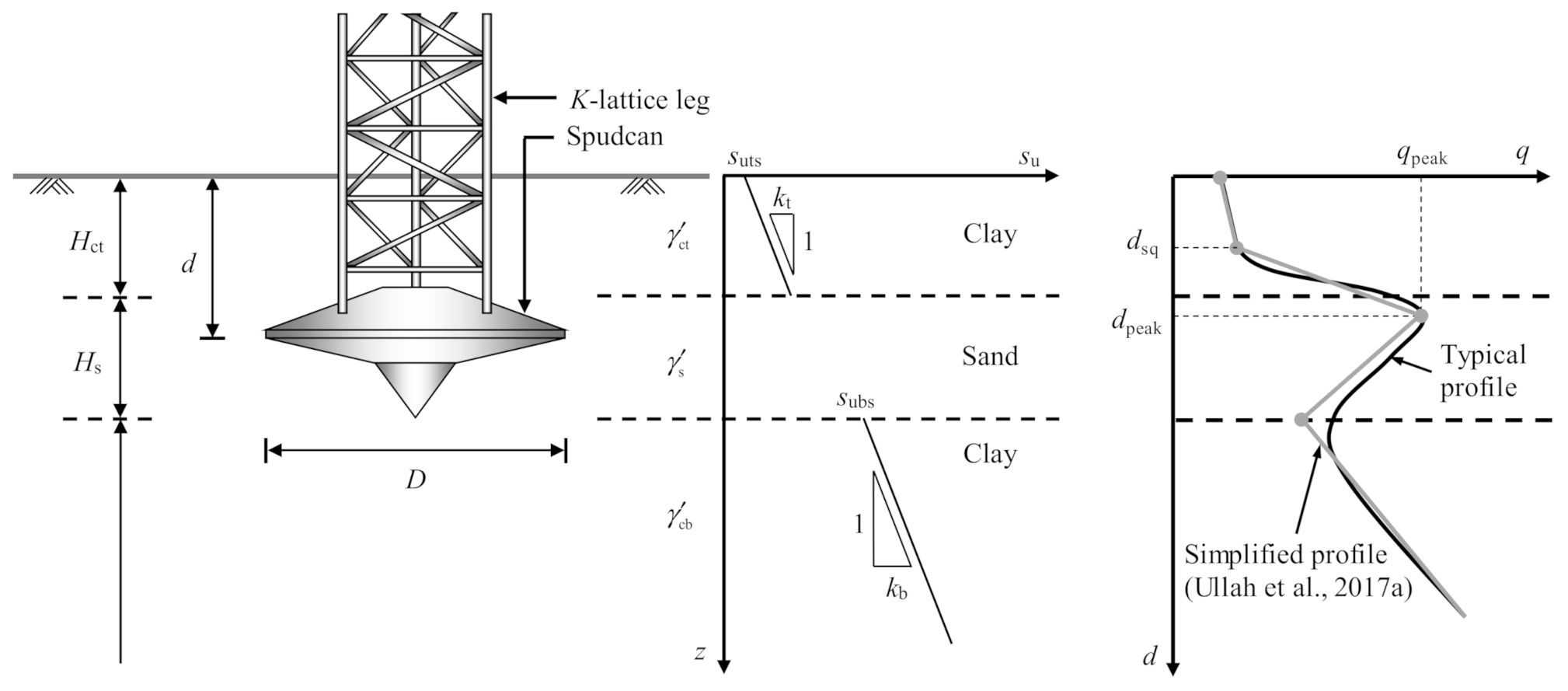
2.1. Soil Parameters

A schematic diagram of a spudcan of diameter D penetrating in clay–sand–clay deposits is illustrated in Figure 1. The sand layer with effective unit weight ${{\gamma }^{\prime }}_{\mathrm{s}}$ and thickness H_s, is interbedded by clay layers. The top clay layer has an effective unit weight of ${{\gamma }^{\prime }}_{\mathrm{ct}}$, undrained shear strength of s_uts at the mudline, strength gradient of k_t and thickness of H_ct. The bottom clay layer has an effective unit weight of ${{\gamma }^{\prime }}_{\mathrm{cb}}$, undrained shear strength of s_ubs at the sand-clay interface, strength gradient of k_b and nominally infinite depth.

2.2. Modified Predictive Model

The predictive model proposed by Ullah et al. [4] has been validated against the centrifuge tests reported by Ullah et al. [19] and Hossain [1]. Based on the geometries and soil parameters summarized in

Table 1. Geometries and soil properties for centrifuge tests considered for parameter optimization [1,19].

Test	D (m)	1st Layer Clay				2nd Layer Sand				3rd Layer Clay
		Hct (m)	suts (kPa)	kt (kPa/m)	${{\mathit{\gamma }}^{\prime }}_{\mathbf{ct}}(\mathbf{kN}/{\mathbf{m}}^3)$	Hs (m)	Relative Density	Critical State Friction Angle	${{\mathit{\gamma }}^{\prime }}_{\mathbf{s}} (\mathbf{kN}/{\mathbf{m}}^3)$	subs (kPa)	kb (kPa/m)	${{\mathit{\gamma }}^{\prime }}_{\mathbf{cb}} (\mathbf{kN}/{\mathbf{m}}^3)$
T1SP	6	2.38	4.9	1.9	6.85	4	74%	31°	10.6	25.6	2.5	7.32
T2SP	6	4.32	4.5	1.6	6.85	4	74%	31°	10.6	27	2.5	7.32
T3SP	6	5.47	4.1	1.5	6.85	4	74%	31°	10.6	26	2.3	7.32
T5SP	6	3.44	4.7	1.7	6.85	2	74%	31°	10.6	18.2	2	7.32
T6SP	6	4.35	4.5	1.6	6.85	6	74%	31°	10.6	26	2.3	7.32
SPa16	16	6.42	0.2	0.5	6.61	6.25	51%	31°	10.14	22.6	2.2	7.63
SPa14	14	6.42	0.2	0.5	6.61	6.25	51%	31°	10.14	22.6	2.2	7.63
SPa12	12	6.42	0.2	0.5	6.61	6.25	51%	31°	10.14	22.6	2.2	7.63
SPa10	10	6.42	0.2	0.5	6.61	6.25	51%	31°	10.14	22.6	2.2	7.63
SPa6	6	6.42	0.2	0.5	6.61	6.25	51%	31°	10.14	22.6	2.2	7.63
SPb16	16	6.32	0.2	0.5	6.61	4	51%	31°	10.14	24.6	2.4	7.63
SPb12	12	6.32	0.2	0.5	6.61	4	51%	31°	10.14	24.6	2.4	7.63
SPb8	8	6.32	0.2	0.5	6.61	4	51%	31°	10.14	24.6	2.4	7.63
SPb6	6	6.32	0.2	0.5	6.61	4	51%	31°	10.14	24.6	2.4	7.63
SPc16	16	4	0.3	0.58	6.61	4	51%	31°	10.14	23	2.5	7.63
SPc8	8	4	0.3	0.58	6.61	4	51%	31°	10.14	23	2.5	7.63
SPc6	6	4	0.3	0.58	6.61	4	51%	31°	10.14	23	2.5	7.63
FS12	6	3.7	0.5	0.75	7.1	1.5	89%	34°	11	4.4	0.75	7.1
FS13	6	3.7	0.5	0.75	7.1	2	89%	34°	11	4.775	0.75	7.1
FS14	6	3.7	0.5	0.75	7.1	4	89%	34°	11	6.275	0.75	7.1

, the peak resistances can mostly be predicted with an error bounded by ±20%, as shown in Figure 2 (solid grey circles) in terms of the ratio r between predicted and measured peak resistances. For the conciseness of the narration, the mathematic framework of Ullah et al.’s [4] method is provided in Appendix A. The predictive model proposed in this study is modified from Ullah et al. [4] so that the soil failure mechanism is modeled more realistically. The modifications include four aspects, which are detailed as follows.

2.2.1. Distribution Factor D_F

Zheng et al. [20] reported that the peak resistances were significantly overestimated for sand overlying clay with high undrained shear strength using the distribution factors estimated by Equation (A3). They have hence collected centrifuge test data from existing publications, carried out additional centrifuge tests and LDFE analyses, and proposed a new design formula for D_F, which is expressed as

$$D_{\mathrm{F}}=0.6{\left(\frac{\left(0.1{{\gamma }^{\prime }}_{\mathrm{cb}}+k_{\mathrm{b}}\right)D}{s_{\mathrm{ubs}}}\right)}^{0.2}{\left(\frac{H_{\mathrm{s}}}{D}\right)}^{-0.4} \mathrm{for} 0.16\le \frac{H_{\mathrm{s}}}{D}\le 1.0$$

(1)

The new formula covers a more comprehensive range of soil properties and geometries, and provides an improved performance for the prediction of peak resistance in sand-over-clay deposits by Hu et al.’s [7] method, based on which Ullah et al.’s [4] model was developed. Therefore, it is also adopted in the modified predictive model of this study.

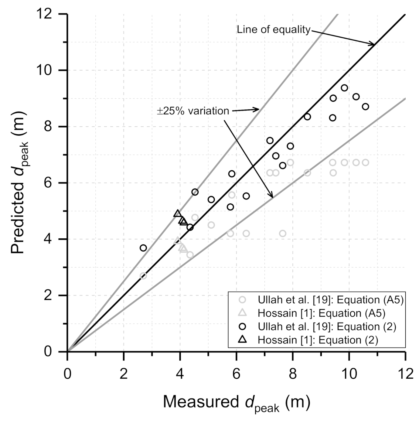
2.2.2. Peak Resistance Depth d_peak

By plotting the measured d_peak from all the related centrifuge tests reported by Ullah et al. [19] and Hossain [1] against the predictions from Equation (A5) of Appendix A, as shown in Figure 3, it is found that the formula tends to underestimate d_peak. The measured values of d_peak from centrifuge tests can be better fitted by

$$\frac{d_{\mathrm{peak}}}{D}=1.04{\left(\frac{H_{\mathrm{ct}}}{D}\right)}^{0.72}+0.12\frac{H_{\mathrm{s}}}{D}$$

(2)

For H_ct = 0, Equation (2) reduces to d_peak = 0.12H_s for sand-over-clay deposits. The comparison between the measured and predicted d_peak for Equation (2) is also plotted in Figure 3, which shows improvement in the estimations.

2.2.3. Soil Resistances from the Sand Plug

With Equation (2) being used and with the assumption that the thickness of the trapped clay frustum is H_c = 0.07H_ct following Ullah et al. [4,19], the effective sand layer height measured from the top of the sand plug to the original sand-clay interface, H_eff, is changed from 0.88H_s to

$$\frac{H_{\mathrm{eff}}}{D}=0.93\frac{H_{\mathrm{ct}}}{D}-1.04{\left(\frac{H_{\mathrm{ct}}}{D}\right)}^{0.72}+0.88\frac{H_{\mathrm{s}}}{D}$$

(3)

By substituting Equation (3) into Equation (A1) with the rest of the design formulas, the same as Ullah et al. [4], the resulting peak resistance ratios are shown as crosses in Figure 2. It is seen that most of the peak resistances are overly underestimated, with the largest error of −44.5%. This is because, for d_peak from Equation (2), the spudcan has penetrated into the sand layer by a depth that the sand-bottom clay interface can no longer be regarded as undeformed. Instead, this deformed interface, which forms the bottom end of the soil plug, protrudes into the bottom clay layer. This is evidenced by Figure 11 of Ullah et al. [19] and Figures 11 and 17a of Hossain [1], which demonstrate the digital images taken from half-model centrifuge tests. Additional resistance is provided by the soil plug below the original sand-bottom clay interface, which contributes an important portion of the peak resistance.

Based on the above failure mechanism, the predictive model by Ullah et al. [4] is modified to incorporate the effects of the soil plug below the original sand-bottom clay interface, as illustrated in Figure 4a. According to the equilibrium of the thin disc element, Equation (A1) can still be used to calculate q_peak. However, the term N_c0s_ubs, which is equal to the vertical stress within the sand frustum at z = H_eff, has to be modified to consider the base and frictional resistances provided by the sand plug with a height of H_plug3 in the bottom clay layer. As such, the vertical equilibrium is established according to Figure 4b for the sand frustum in the bottom clay layer, with the assumption that the shear stress on the periphery is constant and equal to the average undrained shear strength s_u,plug3 of the clay around the frustum

$$N_{\mathrm{c}0}{s}_{\mathrm{ubs}}\frac{\pi D_1^2}{4}=q_{\mathrm{plug}}\frac{\pi D_2^2}{4}+s_{\mathrm{u},\mathrm{plug}3}\cos \psi {\displaystyle {\int }_0^{H_{\mathrm{plug}3}}\pi \left(D_1+2z^{\prime }\tan \psi \right)\frac{\mathrm{d}{z}^{\prime }}{\cos \psi }}$$

(4)

which can be transformed to

$$N_{\mathrm{c}0}{s}_{\mathrm{ubs}}=q_{\mathrm{plug}}{\left(\frac{D_2}{D_1}\right)}^2+\frac{4H_{\mathrm{plug}3}\left(D_1+H_{\mathrm{plug}3}\tan \psi \right)s_{\mathrm{u},\mathrm{plug}3}}{D_1^2}$$

(5)

In Figure 4, D₁, D₂, and H_plug3 are the upper base diameter, lower base diameter, and height of the sand frustum in the bottom clay layer, respectively; and q_plug is the vertical resistance acting on the lower base of the frustum due to soil shearing. To determine these parameters, Test T3SP, as reported by Ullah et al. [19], was reproduced using the LDFE approach in Zheng et al. [5]. Similar to the finding by Zheng et al. [5], a reasonable agreement between the measured and computed penetration resistance profiles is obtained, as shown in Figure 5a. As for the soil plug heights, which are compared in Figure 5b, the total plug height of about 0.05H_ct + 0.9H_s is found from the numerical analysis, close to 0.07H_ct + 0.9H_s reported and assumed by Ullah et al. [4,19]. Therefore, a trapped clay height of H_c = 0.07H_ct and a sand plug height, which is the summation of H_eff and H_plug3, of 0.9H_s are also assumed in this study, and hence the parameters in Equation (5) can be calculated as:

$$D_1=D+2\left(H_{\mathrm{ct}}+H_{\mathrm{s}}-d_{\mathrm{peak}}\right)\tan \psi$$

(6)

$$D_2=D+2\left(H_{\mathrm{ct}}+H_{\mathrm{s}}-d_{\mathrm{peak}}+H_{\mathrm{plug}3}\right)\tan \psi$$

(7)

$$H_{\mathrm{plug}3}=d_{\mathrm{peak}}-0.93H_{\mathrm{ct}}-0.1H_{\mathrm{s}}$$

(8)

$$s_{\mathrm{u}, \mathrm{plug}3}=s_{\mathrm{ubs}}+0.5k_{\mathrm{b}}{H}_{\mathrm{plug}3}$$

(9)

The plug end resistance q_plug can be calculated by multiplying the bearing capacity factor by the corresponding undrained shear strength. The design formula recommended by ISO [21], which considers the embedment depth and soil non-homogeneity after Skempton [22] and Young et al. [23], respectively, is adopted to calculate q_plug as

$$q_{\mathrm{plug}}=6\left[1+0.2\frac{H_{\mathrm{ct}}+H_{\mathrm{s}}+H_{\mathrm{plug}3}}{D_2}\right]\left[s_{\mathrm{ubs}}+k_{\mathrm{b}}\left(H_{\mathrm{plug}3}+0.25D_2\right)\right]$$

(10)

The effects of the bearing capacity depth factor and protruded soil plug in the bottom clay layer are captured through Equation (5) in combination with Equations (6)–(10). The modified predictive model hence estimates the peak resistance according to Equations (A1) and (A2) with D_F from Equation (1), H_eff from Equation (3) and N_c0s_ubs from Equation (5).

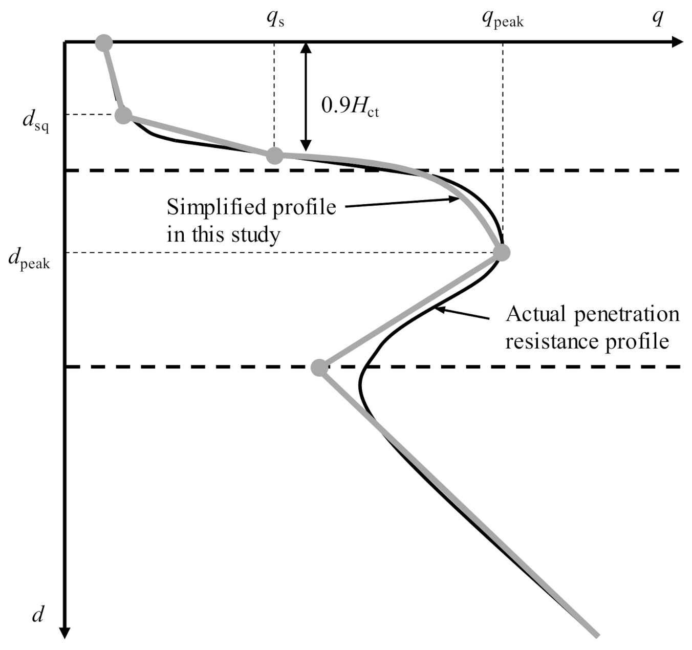
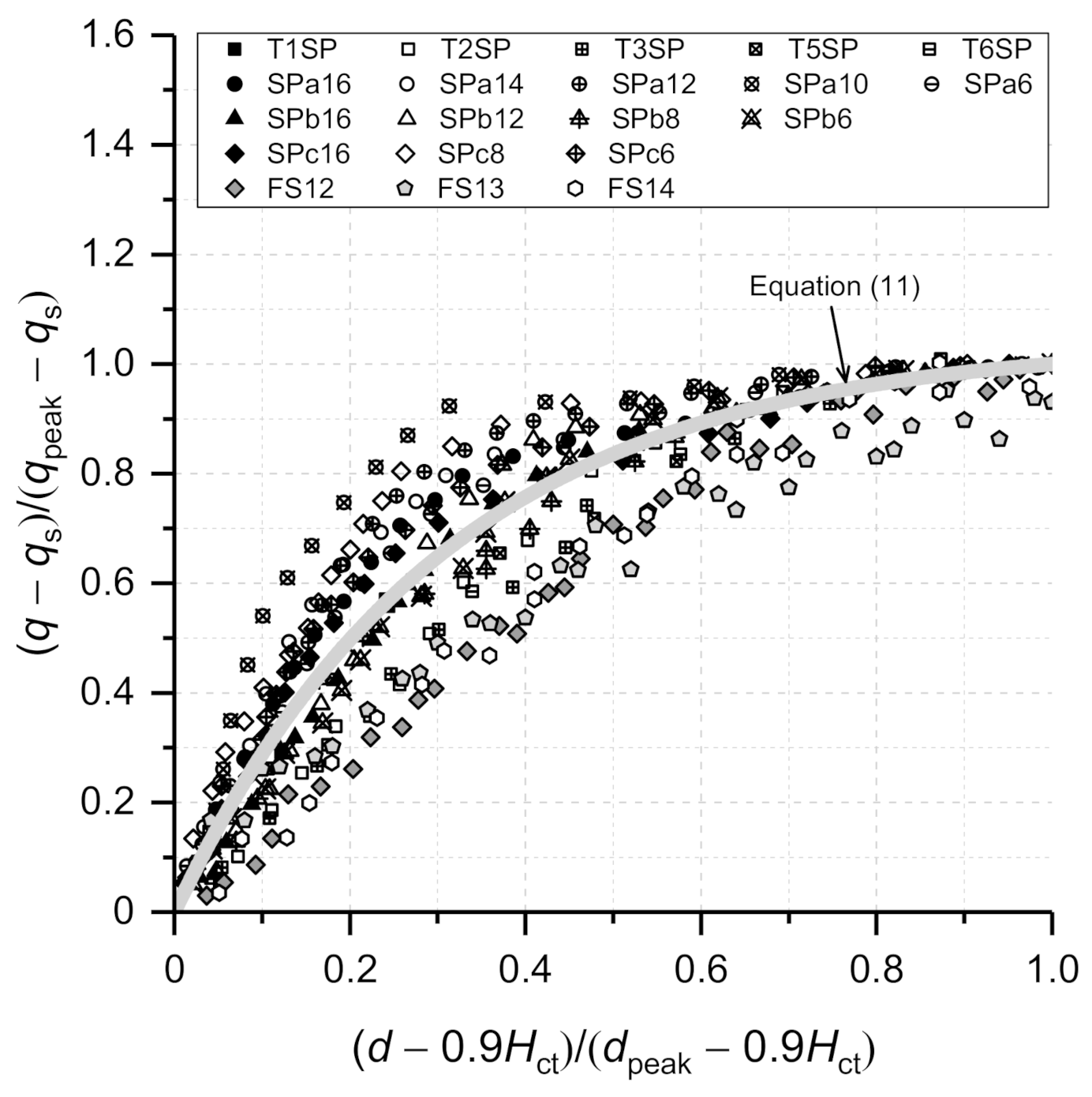
2.2.4. Non-Linear Load-Penetration Response before Peak

The squeezing response was simplified as a straight line by Hu et al. [7] and Ullah et al. [4]. This is acceptable in the deterministic models as the penetration resistance prior to the peak is non-crucial to the assessment of punch-through. However, this curve has to be described appropriately for the application of POT in optimizing the prediction of peak resistance [18]. A non-linear curve is thus proposed to model the load-penetration response between d = 0.9H_ct and d_peak, as shown in Figure 6. According to the centrifuge test data reported by Ullah et al. [19] and Hossain [1], it is found that an exponential function may be used to approximate the non-linear response as

$$\frac{q-q_{\mathrm{s}}}{q_{\mathrm{peak}}-q_{\mathrm{s}}}=A-A{\left(1-1/A\right)}^{\frac{d-0.9H_{\mathrm{ct}}}{d_{\mathrm{peak}}-0.9H_{\mathrm{ct}}}} \mathrm{for} 0.9H_{\mathrm{ct}}\le d\le d_{\mathrm{peak}}$$

(11)

where q_s is the penetration resistance at d = 0.9H_ct and A is a parameter that is best fitted as A = 1.04. The comparison between Equation (11) and the centrifuge data is plotted in Figure 7. For deterministic predictions, the value of q_s can be estimated based on a linear interpolation between the resistances at d_sq and d_peak.

3. Application of POT for Spudcan in Clay–Sand–Clay Deposits

The methodology of POT is based on the data assimilation theory, which is a particular application of Bayes’ theorem [24]. It provides a real-time optimization for the prediction by “adjusting” the model parameters based on the observational information of the variables (e.g., penetration resistance in this study). The technique has been widely incorporated in the forecast models of earth systems [25,26,27,28,29,30,31,32]. The steps for the implementation of POT are summarized in Appendix B.

3.1. POT Scheme for q_peak in Clay–Sand–Clay

Optimized estimation of q_peak in sand over clay deposits was proposed by Jiang et al. [18], in which POT was performed based on the penetration resistances observed at depths of 0–0.025H_s below the sand surface. A straight line was used to simplify the load-penetration response above d_peak. However, this may not be appropriate for clay–sand–clay deposits since the load-penetration response before peak resistance is much more non-linear, with the gradient reducing as the spudcan approaches d_peak. Therefore, a more reasonable description, e.g., Equation (11), should be adopted. Moreover, the observation locations selected by Jiang et al. [18] are below the sand surface and close to d_peak, while an earlier optimization of the predicted peak resistance is preferred, which allows the rig operator to make a judgment as early as possible about whether a punch-through incident will occur or not for spudcans under the designated preload.

For the deterministic model of spudcan in clay–sand–clay deposits introduced in Section 2.2, it is suggested in this study that the observation locations above the top clay–sand interface are adopted so that the prediction of q_peak can be optimized before punch-through occurs. Here, observation locations at d = 0.925, 0.95, 0.975, and 1.0H_ct are selected to verify the performance of the proposed POT in Section 4. With q_s measured at d = 0.9H_ct and the penetration resistance profile estimated from Equation (11) of the modified predictive model, POT can then be performed at the selected observation locations. As justified by Jiang et al. [18], among the model parameters that are determined with relatively significant uncertainties, the most dominant parameter for q_peak in sand overlying clay is the undrained shear strength at the sand-clay interface. A similar phenomenon was found in the trial calculations for clay–sand–clay deposits. Therefore, only s_ubs is adopted as the parameter to be optimized in order to rectify all the uncertainties associated with the prediction of q_peak.

3.2. Procedure of Application

For a modern jack-up rig with the ability to monitor applied vertical load and corresponding spudcan penetration depth during the installation stage, the modified predictive model can be combined with the POT scheme to provide real-time optimization for the prediction of spudcan peak resistance in clay–sand–clay deposits. The detailed procedure is proposed and illustrated in Figure 8, which is summarized as follows:

(1)

Carry out an assessment of punch-through before jack-up installation by making a deterministic prediction of q_peak according to the modified predictive model, i.e., Equations (A1), (A2), (3) and (5)–(10) with D_F from Equation (1). Note that D_F from Equation (1) is only applicable for 0.16 ≤ H_s/D ≤ 1.0. If the designated preload is much lower than the predicted q_peak, e.g., less than 0.75q_peak, POT may not be necessary as the spudcan is highly likely to rest in the top clay layer. However, caution should still be exercised, especially when the spudcan continues to approach the top clay–sand interface with the increase of ballast water.

(2)

Lower the jack-up legs to the seabed and commence the installation. Arrange and apply the load increments carefully to make the spudcan approach the depth of d = 0.9H_ct. If the preload is fully applied before the spudcan reaches the depth of d = 0.9H_ct, POT is not required for optimization. Otherwise, record the observed penetration resistance q_s at the depth of d = 0.9H_ct.

(3)

Generate the parameter ensemble of s_ubs to be optimized, which comprises 10,000 random values with the expectation selected as the value used in the deterministic prediction and the standard deviation (SD) ${\sigma }_{V,\mathrm{M}}$ taken as 20% of the expected value.

(4)

Add more ballast water carefully to jack the spudcan down further (e.g., by an increment of 0.025H_ct or smaller), and record the current vertical load q and the resulted penetration depth d. The recorded load (i.e., penetration resistance) serves as the observed value V_O in Equation (A6) of Appendix B, and its SD is set as ${\sigma }_{V,\mathrm{O}}=0.001V_{\mathrm{O}}$ [18].

(5)

Evaluate the model ensemble of q at the observation location according to Equation (11), in which q_s is obtained from Step 2, d_peak from Equation (2) and q_peak from the modified predictive model with the parameter s_ubs from the parameter ensemble generated in Step 3. Each member in the model ensemble serves as the model prediction in Equation (A6), and the mean and SD of the model ensemble are $\overline{V_{\mathrm{M}}}$ and ${\sigma }_{V,\mathrm{M}}$, respectively.

(6)

Obtain the observational increments according to Equation (A6) based on the variable values determined in Steps 4 and 5, and update the parameter ensemble according to the increments calculated from Equation (A7).

(7)

Optimize the prediction of q_peak using the mean value of the updated parameter ensemble obtained in Step 6.

(8)

Repeat Steps 4–7 to make real-time judgments about whether punch-through will occur or not, and adjust the operation plan accordingly.

Due to the promising convergent rate of POT, the above procedure can be implemented within seconds through, e.g., object-oriented programming languages. This enables real-time optimization in practice for the prediction of the spudcan peak resistance in clay–sand–clay deposits.

4. Performance of the Proposed Approach

4.1. Performance of Modified Predictive Model

The peak resistance ratios resulting from the deterministic predictions of the modified predictive model are plotted as triangles in Figure 2 for the centrifuge tests in Table 1. At first glance, both the modified predictive model and the original one by Ullah et al. [4] show similar performances, resulting in prediction errors mostly within ±20%. However, the statistics summarized in

Table 2. Statistics for the performance of different predictive models.

Predictive Model	Design Formulas	Peak Resistance Ratio, r			MAE *
		Min.	Max.	SD
Ullah et al. [4]	Equations (A1) and (A2) with DF from Equation (A3), Heff = 0.88Hs and Nc0subs from Equation (A4)	0.732	1.267	0.126	9.7%
Figure 4 in this study	Equations (A1) and (A2) with DF from Equation (1), Heff from Equation (3) and Nc0subs from Equation (5)	0.770	1.101	0.094	8.3%

* MAE = Σ|r − 1| divided by the number of centrifuge tests.

indicate an improved performance of the modified predictive model, with the SD and mean absolute error (MAE) reducing from 0.126 to 0.094 and 9.7 to 8.3%, respectively. The peak resistance ratios resulting from the modified predictive model also fell into a narrower range of 0.77–1.101, compared with the range of 0.732–1.267 from Ullah et al.’s [4] approach. This is because the modified predictive model is a more realistic representation of the true soil failure mechanism at peak resistance. Additionally, it also provides the basis for the application of POT in clay–sand–clay deposits.

4.2. Performance of POT

Following the procedure developed in Section 3.2, the proposed POT is used to optimize the prediction of peak resistance for spudcan penetration in clay–sand–clay deposits. Although there are a number of case histories reported by the joint industry project InSafeJIP [3], the recorded load-penetration data were either terminated before the peak resistance or incomplete for the application of POT. Therefore, only centrifuge tests listed in Table 1 are considered, which are all the centrifuge tests available in the existing publications. As mentioned previously, the observation locations in each test are selected at d/H_ct = 0.925, 0.95, 0.975, and 1.0.

4.2.1. Overall Performance

After probabilistic analyses with POT at all observation locations, the absolute errors of the peak resistance ratios are plotted in Figure 9 to compare with results from the corresponding deterministic predictions. Improved predictions of q_peak are observed for most cases, especially for those with relatively large errors from deterministic predictions. However, a relatively obvious increase in the absolute error is also observed in three centrifuge tests, i.e., Tests SPb6, SPb8, and SPb12, with |r − 1| increasing from 3.7, 3.8, and 1% to 19.7, 9.1, and 9.7% respectively. This may be because the modified predictive model is still somewhat biased due to simplifications (e.g., the idealized shape of the soil plug and the simplified representation of the load-penetration squeezing response), despite the modifications proposed in this study. Nevertheless, the absolute errors mostly drop below 10% after the optimization of POT. The overall performance of POT is quantified in

Table 3. Statistics for peak resistance ratios after parameter optimization.

Predictive Model	Design Formulas	Peak Resistance Ratio, r			MAE *
		Min.	Max.	SD
Figure 4 in this study	Equations (A1) and (A2) with DF from Equation (1), Heff from Equation (3) and Nc0subs from Equation (5)	0.803	1.127	0.075	5.9%

* MAE = Σ|r − 1| divided by the number of centrifuge tests.

, where the statistics for the peak resistance ratios after the optimization at all observation locations are listed. Compared with the data in Table 2, the overall performance is further improved, with the SD and MAE of the peak resistance ratios reducing from 0.094 and 8.3% to 0.075 and 5.9%, respectively.

4.2.2. Discussions

Four centrifuge tests, i.e., Tests SPc16, SPb16, T6SP, and SPb6 reported by Ullah et al. [19], are taken as examples to illustrate the optimization process and effectiveness. For each case, the optimized prediction of the penetration resistance profile at each observation location are compared with the centrifuge test result and deterministic prediction in Figure 10. The variations of the ensemble spread (i.e., SD), ensemble mean and experimental value for s_ubs, and the measured and predicted penetration resistances at different observation locations are listed in

Table 4. Variations of data during the process of parameter optimization for Test SPc16.

Centrifuge Test	Type of Variable	Observation Location
		0.925Hct	0.95Hct	0.975Hct	Hct
SPc16	SD of parameter ensemble subs (kPa)	0.32	0.16	0.10	0.07
	Mean of parameter ensemble subs (kPa)	23.8	24.6	25.3	26.1
	Experimental value of subs (kPa)	23.0
	Deterministic prediction of q (kPa)	251.2	269.4	285.7	300.4
	Optimized prediction of q (kPa)	286.7	303.1	319.0	334.4
	Measured q (kPa)	286.6	303.3	320.1	336.8
	Deterministic prediction of qpeak (kPa)	421.1
	Optimized prediction of qpeak (kPa)	427.0	433.5	439.8	446.0
	Measured qpeak (kPa)	486.7

,

Table 5. Variations of data during the process of parameter optimization for Test SPb16.

Centrifuge Test	Type of Variable	Observation Location
		0.925Hct	0.95Hct	0.975Hct	Hct
SPb16	SD of parameter ensemble subs (kPa)	0.22	0.11	0.07	0.06
	Mean of parameter ensemble subs (kPa)	23.3	24.5	25.7	26.9
	Experimental value of subs (kPa)	24.6
	Deterministic prediction of q (kPa)	264.3	291.0	313.6	342.1
	Optimized prediction of q (kPa)	275.6	301.5	326.2	349.7
	Measured q (kPa)	275.6	302.5	329.4	356.2
	Deterministic prediction of qpeak (kPa)	439.6
	Optimized prediction of qpeak (kPa)	428.6	438.9	448.9	458.8
	Measured qpeak (kPa)	519.6

,

Table 6. Variations of data during the process of parameter optimization for Test T6SP.

Centrifuge Test	Type of Variable	Observation Location
		0.925Hct	0.95Hct	0.975Hct	Hct
T6SP	SD of parameter ensemble subs (kPa)	0.38	0.19	0.12	0.09
	Mean of parameter ensemble subs (kPa)	43.7	44.3	44.7	45.1
	Experimental value of subs (kPa)	26.0
	Deterministic prediction of q (kPa)	583.9	654.8	712.8	760.2
	Optimized prediction of q (kPa)	1182.8	1198.2	1212.6	1226.1
	Measured q (kPa)	1183.5	1199.1	1214.8	1230.4
	Deterministic prediction of qpeak (kPa)	953.9
	Optimized prediction of qpeak (kPa)	1246.3	1255.5	1262.2	1268.7
	Measured qpeak (kPa)	1238.7

, and

Table 7. Variations of data during the process of parameter optimization for Test SPb6.

Centrifuge Test	Type of Variable	Observation Location
		0.925Hct	0.95Hct	0.975Hct	Hct
SPb6	SD of parameter ensemble subs (kPa)	0.07	0.04	0.03	0.03
	Mean of parameter ensemble subs (kPa)	7.7	9.5	11.7	13.7
	Experimental value of subs (kPa)	24.6
	Deterministic prediction of q (kPa)	442.5	519.0	570.1	604.2
	Optimized prediction of q (kPa)	293.0	355.4	412.1	461.9
	Measured q (kPa)	290.3	362.8	435.3	507.8
	Deterministic prediction of qpeak (kPa)	659.0
	Optimized prediction of qpeak (kPa)	434.4	455.9	483.2	510.2
	Measured qpeak (kPa)	635.4

. There are some interesting points to note in Figure 10 and Table 4, Table 5, Table 6, Table 7, as discussed below.

While the proposed approach does not work perfectly for all cases, Tests SPc16 and SPb16 are representative cases in terms of the variations of optimized resistance profile and parameter ensemble with the observation location. As shown in Figure 10a,b, the optimized penetration resistance profile evolves towards the measured profile along with the spudcan penetration after the first observation location, providing greater confidence in the assessment of punch-through. The best performance is observed for Test T6SP (Figure 10c), where the absolute error reduces from 23.0% to 2.4% after the optimization at all observation locations. This may reflect the relatively large experimental error in the measurement of s_ubs for Test T6SP. For these three cases where POT leads to an improved prediction, the statistics in Table 4, Table 5, Table 6 demonstrate a consistent trend: after the first observation location, the variation of s_ubs is evolutionary (by less than 5% after each optimization), and the lower degree of variation is associated with better performance; the optimized q at each observation location is close to the measured value, with errors less than 1%.

However, it should be noted that for cases where the POT has resulted in an improved prediction of q_peak, the optimized resistance profile does not necessarily evolve towards the measured data all the way as the spudcan approaches the d_peak. For example, in Test SPb16 (Figure 10b), the optimization of q_peak at d = 0.925H_ct results in a profile that is even further away from the measured data, although the following optimized profiles gradually get closer to the measured data as the spudcan penetrates further and leads to a smaller predictive error after all observation locations. Test T6SP is another example (Figure 10c), where the discrepancy between the optimized and measured penetration resistance profiles gets larger after each observation location. Nevertheless, the optimized penetration resistance profile gets very close to the measured data immediately at the first observation location (i.e., d = 0.925H_ct), and its changes in the following observation locations are quite negligible (less than 2%).

The worst performance of POT is observed for Test SPb6 (Figure 10d). Table 7 shows that at the first observation location of d = 0.925H_ct, there is a sharp change in s_ubs from 24.6 to 7.7 kPa and the predictive error of q_peak changes from 3.7% to −31.6%, although the optimized prediction of q becomes almost identical to the observed value with the updated s_ubs. At subsequent observation locations, the optimized resistance profiles evolve towards the measured data, but the variation in s_ubs is still significant (by ~20% after each optimization), and the gap between the optimized and observed values of q also grows with the penetration depth, with a difference of about 9% (461.9 vs. 507.8 kPa) at the last observation location. This is in contrast to the cases that show an improved prediction with POT, where the variation in s_ubs is evolutionary and the optimized and observed values of q only have a minimal difference. The main reason may be because the simplified non-linear curve is not a good representation for the squeezing response of Test SPb6.

The different patterns of variations discussed above lead to the following implications for the practical application of the proposed POT approach: (a) an evolutionary variation of the optimized s_ubs (e.g., by <5%) and a close agreement between the optimized and measured q values usually indicate an improved prediction of q_peak; and (b) extreme cautions should be taken during the optimization process if the variation of the optimized s_ubs is significant (e.g., by >5%) and there is an increasing error between the optimized and measured q values, which, although rare, may indicate a worsened prediction by POT.

5. Conclusions

This paper describes a modified predictive model for assessing the peak resistance of spudcan in clay–sand–clay deposits. Model modifications mainly include the incorporation of the effects of the bearing capacity depth factor and the protruded soil plug in the bottom clay layer. The modified model provides a more realistic representation for the true soil failure mechanism at punch-through, and the verification against existing centrifuge tests shows an improved performance compared with the original model. Based on the modified predictive model, the parameter optimization technique has been employed to optimize the prediction of peak resistance in clay–sand–clay deposits using the penetration resistances observed at locations above the top clay–sand interface. A detailed procedure for applying the parameter optimization technique has been summarized and then applied to the centrifuge tests. Further improvement on the prediction of peak resistance has been demonstrated compared with the deterministic predictions from the modified predictive model, which confirms the effectiveness of the proposed approach. Discussions have been made on the optimization process in terms of the variations of the parameter ensemble and the optimized penetration resistances. Based on the discussions, some guidelines for the application of the proposed approach have been suggested.

References

1. Hossain, M.S. Experimental investigation of spudcan penetration in multi-layer clays with interbedded sand layers. Géotechnique 2014, 64, 258–276. [Google Scholar] [CrossRef]
2. Zheng, J.; Hossain, M.S.; Wang, D. Numerical modeling of spudcan deep penetration in three-layer clays. Int. J. Geomech. 2015, 15, 04014089. [Google Scholar] [CrossRef] [Green Version]
3. InSafeJIP. Improved Guidelines for the Prediction of Geotechnical Performance of Spudcan Foundations during Installation and Removal of Jack-Up Units; EOG0574-Rev1c; RPS Energy: Woking, UK, 2011. [Google Scholar]
4. Ullah, S.N.; Stanier, S.; Hu, Y.; White, D.J. Foundation punch-through in clay with sand: Analytical modelling. Géotechnique 2017, 67, 672–690. [Google Scholar] [CrossRef]
5. Zheng, J.; Hossain, M.S.; Wang, D. Numerical investigation of spudcan penetration in multi-layer deposits with an interbedded sand layer. Géotechnique 2017, 67, 1050–1066. [Google Scholar] [CrossRef]
6. Lee, K.K.; Randolph, M.F.; Cassidy, M.J. Bearing capacity on sand overlying clay soils: A simplified conceptual model. Géotechnique 2013, 63, 1285–1297. [Google Scholar] [CrossRef]
7. Hu, P.; Stanier, S.A.; Cassidy, M.J.; Wang, D. Predicting peak resistance of spudcan penetrating sand overlying clay. J. Geotech. Geoenviron. Eng. 2014, 140, 04013009. [Google Scholar] [CrossRef] [Green Version]
8. Hossain, M.S.; Zheng, J.; Menzies, D.; Meyer, L.; Randolph, M.F. Spudcan penetration analysis for case histories in clay. J. Geotech. Geoenviron. Eng. 2014, 140, 04014034. [Google Scholar] [CrossRef]
9. Hossain, M.S.; Hu, P.; Cassidy, M.J.; Menzies, D.; Wingate, A. Measured and calculated spudcan penetration profiles for case histories in sand-over-clay. Appl. Ocean Res. 2019, 82, 447–457. [Google Scholar] [CrossRef]
10. Houlsby, G.T. A probabilistic approach to the prediction of spudcan penetration of jack-up units. In Frontiers in Offshore Geotechnics II, 1st ed.; Gouvenec, S., White, D., Eds.; CRC Press: Boca Raton, FL, USA, 2010; pp. 673–678. [Google Scholar]
11. Cassidy, M.J.; Li, J.; Hu, P.; Uzielli, M.; Lacasse, S. Deterministic and probabilistic advances in the analysis of spudcan behavior. In Frontiers in Offshore Geotechnics III, 1st ed.; Meyer, V., Ed.; CRC Press: Boca Raton, FL, USA, 2015; pp. 183–212. [Google Scholar]
12. Yi, J.T.; Huang, L.Y.; Li, D.Q.; Liu, Y. A Large-deformation random finite-element study: Failure mechanism and bearing capacity of spudcan in a spatially varying clayey seabed. Géotechnique 2020, 70, 392–405. [Google Scholar] [CrossRef]
13. Li, J.; Tian, Y.; Cassidy, M. Failure mechanism and bearing capacity of footings buried at various depths in spatially random soil. J. Geotech. Geoenviron. Eng. 2015, 141, 1–11. [Google Scholar] [CrossRef] [Green Version]
14. Li, L.; Li, J.; Huang, J.; Gao, F. Bearing capacity of spudcan foundations in a spatially varying clayey seabed. Ocean Eng. 2017, 143, 97–105. [Google Scholar] [CrossRef] [Green Version]
15. Li, L.; Li, J.; Huang, J.; Liu, H.; Cassidy, M.J. The bearing capacity of spudcan foundations under combined loading in spatially variable soils. Eng. Geol. 2017, 227, 139–148. [Google Scholar] [CrossRef]
16. Uzielli, M.; Cassidy, M.J.; Hossain, M.S. Bayesian prediction of punch-through for spudcans in stiff-over-soft clay. In Proceedings of the Geotechnical Safety and Reliability: Honoring Wilson H. Tang, Proceedings of Geo-Risk, Denver, CO, USA, 4–7 June 2017; Juang, C.H., Gilbert, R.B., Zhang, L., Zhang, J., Zhang, L., Eds.; American Society of Civil Engineers: Reston, VA, USA, 2017; pp. 247–265. [Google Scholar]
17. Li, J.; Hu, P.; Uzielli, M.; Cassidy, M.J. Bayesian prediction of peak resistance of a spudcan penetrating sand-over-clay. Géotechnique 2018, 68, 905–917. [Google Scholar] [CrossRef]
18. Jiang, J.; Wang, D.; Zhang, S. Improved prediction of spudcan penetration resistance by an observation-optimized model. J. Geotech. Geoenviron. Eng. 2020, 146, 06020014. [Google Scholar] [CrossRef]
19. Ullah, S.N.; Stanier, S.; Hu, Y.; White, D.J. Foundation punch-through in clay with sand: Centrifuge modelling. Géotechnique 2017, 67, 870–889. [Google Scholar] [CrossRef]
20. Zheng, J.; Chen, Y.; Chen, X.; Wang, D.; Jing, S. Improved prediction of peak resistance for spudcan penetration in sand layer overlying clay. J. Geotech. Geoenviron. Eng. (under review).
21. ISO International Organization for Standardization. Petroleum and Natural Gas Industries—Site Specific Assessment of Mobile Offshore Units—Part 1: Jack-Ups. ISO 19905-1; ISO: Geneva, Switzerland, 2016. [Google Scholar]
22. Skempton, A.W. The Bearing Capacity of Clays; Building Research Congress: London, UK, 1951. [Google Scholar]
23. Young, A.G.; Remmes, B.D.; Meyer, B.J. Foundation performance of offshore jack-up drilling rigs. J. Geotech. Eng. 1984, 110, 841–859. [Google Scholar] [CrossRef]
24. Jazwinski, A.H. Stochastic Processes and Filtering Theory; Academic Press: New York, NY, USA, 1970. [Google Scholar]
25. Evensen, G. Sequential data assimilation with a nonlinear quasi-geostrophic model using Monte Carlo methods to forecast error statistics. J. Geophys. Res. 1994, 99, 10143–10162. [Google Scholar] [CrossRef]
26. Fukumori, I.; Raghunath, R.; Fu, L.; Chao, Y. Assimilation of TOPEX/POSEIDON data into a global ocean circulation model: How good are the results? J. Geophys. Res. 1999, 104, 25647–25665. [Google Scholar] [CrossRef]
27. Annan, J.D.; Hargreaves, J.C.; Edwards, N.R.; Marsh, R. Parameter estimation in an intermediate complexity Earth System Model using an ensemble Kalman filter. Ocean Model. 2005, 8, 135–154. [Google Scholar] [CrossRef]
28. Aksoy, A.; Zhang, F.; Nielsen-Gammon, J.W. Ensemble-based simultaneous state and parameter estimation. Geophys. Res. Lett. 2006, 33, L12801. [Google Scholar] [CrossRef] [Green Version]
29. Kondrashov, D.; Sun, C.; Ghil, M. Data assimilation for a coupled ocean-atmosphere model, Part II: Parameter estimation. Mon Weather Rev. 2008, 136, 5062–5076. [Google Scholar] [CrossRef] [Green Version]
30. Zhang, S. Impact of observation-optimized model parameters on decadal predictions: Simulation with a simple pycnocline prediction model. Geophys. Res. Lett. 2011, 38, 1–5. [Google Scholar] [CrossRef] [Green Version]
31. Zhang, S. A study of impacts of coupled model initial shocks and state-parameter optimization with observations on climate predictions using a simple pycnocline prediction model. J. Clim. 2011, 24, 6210–6226. [Google Scholar] [CrossRef] [Green Version]
32. Zhang, S.; Liu, Z.; Rosati, A.; Delworth, T. A study of enhancive parameter correction with coupled data assimilation for climate estimation and prediction using a simple coupled model. Tellus A Dyn. Meteorol. Oceanogr. 2012, 64, 10963. [Google Scholar] [CrossRef] [Green Version]
33. Houlsby, G.T.; Martin, C.M. Undrained bearing capacity factors for conical footings on clay. Géotechnique 2003, 53, 513–520. [Google Scholar] [CrossRef]
34. Drescher, A.; Detournay, E. Limit load in translational failure mechanisms for associative and non-associative materials. Géotechnique 1993, 43, 443–456. [Google Scholar] [CrossRef]
35. Bolton, M.D. The strength and dilatancy of sands. Géotechnique 1986, 36, 65–78. [Google Scholar] [CrossRef] [Green Version]
Figure 1. Illustration of spudcan in clay–sand–clay deposit and corresponding typical penetration resistance profile.
Jmse 09 00689 g001
Figure 2. Comparison between measured and predicted peak resistances.
Jmse 09 00689 g002
Figure 3. Comparison between measured and predicted depths of peak resistance.
Jmse 09 00689 g003
Figure 4. A modified predictive model for qpeak. (a) Illustration of soil failure mechanism; (b) forces acting on the sand frustum in the bottom clay layer.
Jmse 09 00689 g004
Figure 5. A comparison of experimental and numerical results for Test T3SP of Ullah et al. [19]. (a) Penetration resistance profiles; (b) soil plug heights.
Jmse 09 00689 g005
Figure 6. Illustration of simplified squeezing response.
Jmse 09 00689 g006
Figure 7. Comparison of measured and predicted penetration resistance profiles between d = 0.9Hct and dpeak.
Jmse 09 00689 g007
Figure 8. Flowchart of proposed assessment procedure for optimized estimation of qpeak.
Jmse 09 00689 g008
Figure 9. Performance of proposed approach for optimized assessment of qpeak.
Jmse 09 00689 g009
Figure 10. Variation of predicted penetration resistance profile with the optimization at each observation location. (a) Test SPc16; (b) Test SPb16; (c) Test T6SP; (d) Test SPb6.
Jmse 09 00689 g010