Horizontal Correlation of Long-Range Bottom Reverberation in Shallow Sloping Seabed

Abstract

The performance of active sonar detection systems is seriously affected by the reverberation at the bottom of the waveguide in shallow water. In order to improve the performance of active sonar detection, it is necessary to understand the horizontal correlation of shallow-water bottom reverberation in active towed-array processing technology. However, the current research on the spatial correlation of reverberation is mainly based on vertical correlation, little work has been done on the horizontal correlation characteristics of long-distance seabed reverberation, and there is no support from sea test data. In this paper, the coupled mode reverberation model is applied to the horizontal correlation, and is studied according to the receiving position, time, and frequency. The simulation results show that, for the long-range bottom reverberation, the lateral correlation is greater than the longitudinal correlation in the horizontal space. By introducing the adiabatic mode solution, the mathematical model of horizontal correlation in the range-dependent waveguide with depth is derived. The numerical results show that the influence of the seabed dip angle on the horizontal correlation should be considered and that the horizontal correlation is affected obviously by the propagation effects of the sloped sea floor. Finally, the experimental data processing and analysis are given and verify the correctness of the algorithm.

1. Introduction

As we all know, the reverberation in a shallow-water waveguide seriously affects the performance of the active array system [1,2,3]. In order to improve the detection ability of the active array, it has important scientific significance to study the mechanism and influence mechanism of seafloor reverberation. Regarding the spatial distribution of submarine reverberation, Zhou, J.X. et al. used the normal wave reverberation model to study the vertical correlation of the shallow sea submarine reverberation from the angle spectrum of the normal wave, and discussed the use of vertical correlation to invert the bottom parameters. The influence of sea surface undulation on the vertical correlation characteristics of the seafloor reverberation, and the influence of the vertical correlation change of the seafloor reverberation caused by the undulating sea surface scattering on the uncertainty of the inversion of seafloor parameters, were analyzed [4,5]. By using the data collected by horizontal array, a rapid environmental assessment mechanism was developed by Preston, and the distribution of scattering intensity was obtained according to the seabed reverberation data [6]. The vertical correlation is discussed by Li Fenghua, and the relationships between the vertical correlations of reverberation with reverberation time, frequency, receiver depth, and seabed parameters were also studied. Moreover, a method of inversion for bottom reflection loss and bottom scattering strength was put forward by using reverberation intensity and vertical correlation coefficients [7]. It can be seen that many researchers have used the normal wave reverberation model and the angular spectrum analysis model to conduct in-depth research on the vertical correlation characteristics of the seabed reverberation and the inversion of seabed parameters based on the vertical correlation, and the research focuses are almost for the vertical correlation of shallow sea reverberation in stratified media, where sea depth has nothing to do with horizontal distance [8,9]. There is little research on the characteristics of shallow sea reverberation and shallow sea reverberation levels related to the horizontal distance in the shallow sea transition slope area [10].

During the signal detection process of the active towed array, the horizontal correlation of reverberation has a greater impact on the detection performance. Therefore, studying the horizontal correlation of reverberation is of great significance for improving the signal processing gain of the active towed array [11,12,13]. However, at present, researchers mainly do the vertical correlation of reverberation intensity, and there is little theoretical work on horizontal correlation, let alone effective data support [14]. Secondly, the discussion of the correlation of the reverberation level in the transitional sea area needs to give the remote reverberation model of the transitional sea area. Although there are theoretical models in this aspect, only the intensity prediction of the remote reverberation is concerned [15]. At present, there is almost no research on the horizontal correlation characteristics of the theoretical framework of the remote reverberation model, especially the research on the correlation characteristics of the reverberation level in the transitional sea area [16]. In order to solve the above problems, this paper discusses the horizontal correlation characteristics of long-range seabed reverberation in the shallow sea transitional slope area.

To explore such problems, there are two basic issues that need to be solved: first, the reverberation received by the horizontal drag array is not at the same horizontal coordinate received by the emitted sound source, and its basic reverberation model needs to consider the reverberation of the transceiver mode problem. Second, it is necessary to consider the modeling problem of long-range submarine reverberation under the condition of inclined waveguides related to the change of sea depth and the horizontal distance. In the related fields of the above two problems, C. H. Harrison used the concept of a sound ray invariant to derive the rigorous solutions of bistatic target echo, bistatic reverberation, and the signal-to-mix ratio. This theory makes use of the “mode stripping” phenomenon in the propagation process (mode-stripping, the seabed loss caused by the scattering of high-order modal normal waves due to the scattering of large glancing angles, which gradually disappears during the propagation process) [17]. In the case of constant sound velocity, this model can handle long-range reverberation under any distance-related seabed conditions as long as the adiabatic approximation is satisfied, and can be extended to handle bistatic conditions. The formula deduced by this model gives an analytical formula about sea depth, critical angle, and seabed reflection loss, and there is no need to use numerical calculation in the specific calculation process, so the calculation speed is faster [18,19]. Similarly, Li Fenghua and Liu Jianjun extended the normal mode reverberation model in shallow water to the case of inclined seabeds by using the adiabatic normal mode theory [20]. However, none of the above work gives the horizontal correlation characteristics of the seabed reverberation in the shallow slope area. Moreover, most of the above models use Lambert’s theorem based on the empirical scattering function as the scattering description, and lack a physical description of the seafloor scattering process.

In order to improve the existing methods, this paper uses the coupled normal mode reverberation theory based on the first-order perturbation approximation to analyze the spatial correlation characteristics of long-range seafloor reverberation from the perspective of sound propagation and according to the statistical characteristics of the seafloor undulating interface. The advantage of the model is that the reverberation field can be obtained directly by determining the random fluctuation structure of the seabed interface [21,22,23]. At the same time, the model can be extended to the range-dependent shallow-water transition area to further analyze the reverberation level correlation characteristics of the transition area. The physical meaning is that the reverberation is regarded as the coupling between the incident sound wave and the seabed interface. Its characteristics are as follows: Firstly, the model is directly derived from Green’s theorem, which strictly conforms to the reciprocity theorem in theory. Secondly, on the basis of the physical scattering mechanism, the model can analyze the influence of the waveguide effect and the interface scattering characteristics on the horizontal correlation characteristics of long-range reverberation in shallow water. Section 2 introduces the theoretical model and calculation formula of reverberation level correlation. In Section 3.1, the horizontal correlation characteristics of the seafloor reverberation are analyzed by numerical examples. In Section 3.2, the proposed method is verified by marine experimental data. Finally, the conclusion is given in Section 4.

2. Materials and Methods

For Pekeris waveguide, which is considered to be with a plane sea surface and irregular bottom interface, is described by $H\left(x,y\right)=H_0+\eta \left(x,y\right)$·$\left(\eta <<H_0\right),$ where $H_0$ is the average depth of the water, and $\eta$ is a random quantity with the average value 0. The density and sound speed of the sea water and bottom medium are respectively ${\rho }_1,c_1;{\rho }_2,c_2$. Additionally, $\overrightarrow{r}$ is the position vector on the horizontal plane $\overrightarrow{r}=\left(x,y\right)$. According to the coupled mode reverberation model [24,25], the reverberant field of the point harmonic source could be written as:

$$P(\omega ,\overrightarrow{r},z)={\displaystyle \sum _n\left[{\phi }_{1n}(r)+{\phi }_{2n}(r)\right]Z_n(z,{\xi }_n)}$$

(1)

where $Z_n(z,{\xi }_n)$ are the so-called “local modes”, ${\xi }_n$ is the eigenvalue of the n-th mode, and ${\phi }_{1n}(r),{\phi }_{2n}(r)$ are the incoherent and coherent parts of the horizontal factors for the reverberant field, respectively. Considering only the first-order perturbation factor, corresponding to the bottom reverberation caused by boundary roughness, the horizontal factors would have following forms:

$${\phi }_{1n}(x,y)\approx \frac{i}{4}{\displaystyle \iint -\frac{2{\beta }_{1n}^2}{B_n}\eta {{\psi }^{\prime }}_n(x,y){\psi }_n(x,y)d{x}^{\prime }d{y}^{\prime }}$$

(2)

$${\phi }_{2n}(x,y)\approx \frac{i}{4}{\displaystyle \iint {\displaystyle \sum _m{G}_{mn}(\frac{\partial {{\psi }^{\prime }}_m}{\partial x}\frac{\partial \eta }{\partial x}}+\frac{\partial {{\psi }^{\prime }}_m}{\partial y}\frac{\partial \eta }{\partial y}){{\psi }^{\prime }}_m(x,y){\psi }_n(x,y)d{x}^{\prime }d{y}^{\prime }}$$

(3)

where ${\xi }_n,{\psi }_n(x,y)$ represent the zero-order approximation, respectively, and $G_{nm}$ are the mode-coupling coefficients. Considering the incoherent part only for simplicity and the horizontal factor of the bottom reverberation for the impulsive source, ${\Psi }_{rn}(r)$ can be given by Fourier integral of ${\varphi }_{1n}$.

For example, in an almost layered medium like the Pekeris waveguide with a rough bottom surface, the zero-th order approximation of the transfer function ${\psi }_n(x,y)$ is $H_0^{(1)}({\xi }_{n}r)$. In this case, the horizontal correlation of the scattered field at the two receiving points $(x+\Delta x,\Delta y)$ and $(x-\Delta x,-\Delta y)$ can be evaluated by the horizontal factor ${\Psi }_{rn}(r)$, where <> means time averaging. The geometry relationship in Equations (4) and (5) is shown in Figure 1.

$$\langle p(t,\hspace{0.17em}{\overrightarrow{r}}_1)p^{\ast }(t,\hspace{0.17em}{\overrightarrow{r}}_2)\rangle ={\displaystyle \sum _n\langle {\Psi }_{1n}(r_1){\Psi }_{1n}^{\ast }(r_2)\rangle }$$

(4)

$${\Psi }_{1n}^{}(r)=-\frac{{\beta }_{0n}\tau }{{\pi }^2{B}_n}\sqrt{\frac{2\pi {\omega }_0}{t}}\exp -i\left(\omega t+\frac{\pi }{4}\right){\displaystyle \underset{{\Omega }_1}{\iint }\frac{\eta ({r^{\prime }}_n)}{\sqrt{{r^{\prime }}_{n}R}}\exp i{\xi }_n\left({r^{\prime }}_n+R_n\right)}d{x}^{\prime }d{y}^{\prime }.$$

(5)

After combining Equation (4) with Equation (5), expanding $\exp i{\xi }_n\left(R_1-R_2\right)$ according to Taylor’s series, and separating the transverse and longitudinal coordinates, we can finally obtain the longitudinal correlation coefficient ${\rho }_{h\hspace{0.17em}L}$ and transverse correlation coefficient ${\rho }_{h\hspace{0.17em}T}$:

$${\rho }_{h\hspace{0.17em}L}\approx {\displaystyle \sum _{n}1-\frac{k^2{\sin }^2{\theta }_n}{4}\left[\Delta x^2{r}_n^3{(r_n{}^2-r_0^2)}^{-\raisebox{1ex}{$3$}\!\left/ \!\raisebox{-1ex}{$2$}\right.}\right]}$$

(6)

$${\rho }_{h\hspace{0.17em}T}\approx {\displaystyle \sum _{n}1-\frac{k^2{\sin }^2{\theta }_n}{4r_0^2}}\left\{\Delta y^2[1+r_n{(r_n{}^2-r_0^2)}^{-\raisebox{1ex}{$1$}\!\left/ \!\raisebox{-1ex}{$2$}\right.}][r_n{}^2-r_n{(r_n{}^2-r_0^2)}^{\raisebox{1ex}{$1$}\!\left/ \!\raisebox{-1ex}{$2$}\right.}]\right\}.$$

(7)

For the range-dependent waveguide with the varying depth $H(x)=H_0(1+\alpha x)\left(1+\eta \right)\approx H_0(1+\alpha x+\eta )$, the zero-th order approximation of the transfer function ${\psi }_n(x,y)$ cannot be written as $H_0^{(1)}({\xi }_{n}r)$. For this situation, when writing ${\psi }_n(x,y)$ as $D_n\exp (i{W}_n)$, it can be evaluated by the adiabatic mode solution in the Cartesian coordinate system.

According to the adiabatic approach, ${\psi }_n(x,y)$ would obey the equation:

$$\frac{{\partial }^2{\psi }_n}{\partial x^2}+\frac{{\partial }^2{\psi }_n}{\partial y^2}+{\xi }_n^2{\psi }_n=0.$$

(8)

Then, ${\psi }_n^{}=D_n\exp (i{W}_n)$ could be written as:

$${(\frac{\partial W_n^{}}{\partial x})}^2+{(\frac{\partial W_n^{}}{\partial y})}^2={\xi }_n^2$$

(9)

$$2\nabla D_n•\nabla W_n+D_n{\nabla }^2{W}_n=0.$$

(10)

In Equation (10), the dot $•$ means the operation of the inner product on the horizontal plane. Then, the coefficient of horizontal correlation in the waveguide with inclined seafloor is

$$\langle p(t,\hspace{0.17em}{\overrightarrow{r}}_1)p^{\ast }(t,\hspace{0.17em}{\overrightarrow{r}}_2)\rangle ={\displaystyle \sum _n\langle {\Psi }_{1n}(r_1){\Psi }_{1n}^{\ast }(r_2)\rangle }$$

(11)

where

$${\Psi }_{1n}^{}(r)\approx \frac{{\tau }^2{\beta }_{sn}^4{c}_1^2}{2\pi f({\xi }_{sn},{\xi }_{rn}){\omega }_{1}t{B}_n^2}{\displaystyle \underset{{\Omega }_1}{\iint }\eta ({r^{\prime }}_n){D^{\prime }}_n(r^{\prime },{\omega }_0)D_n(R,{\omega }_0)\exp i[{W^{\prime }}_n(r^{\prime })+W_n(R)]d{x}^{\prime }d{y}^{\prime }}$$

(12)

Combining Equation (11) with Equation (12), the cross-correlation coefficients for the two receiving points are

$${\displaystyle \sum _n\langle {\Psi }_{1n}(r_1){\Psi }_{1n}^{\ast }(r_2)\rangle }=I(\eta ,\tau ,c_0,t){\displaystyle \sum _n{\displaystyle \underset{{\Omega }_1}{\iint }\exp i\left[W_n(R_1)-W_n(R_2)\right]}d{x}^{\prime }d{y}^{\prime }}$$

(13)

The integral at the right hand of Equation (13) can be evaluated by numerical solution. It is shown that the incoherent cross-correlation between the two hydrophones is evaluated, where $I(\eta ,\tau ,c_0,t)$ denotes the intensity factor. If the two considered receivers are put to one point, and the phase difference is denoted, the integrated part would be neglected. Then, the derivation of the cross-correlation operation would be altered to an expression of reverberation intensity at the receiver point.

3. Results

In this section, the model proposed in this paper is first verified by simulation results, and then the experimental data are processed. The results show that the method proposed in this paper is effective.

3.1. Simulation Results

On the basis of the coupled normal mode wave reverberation theory, the relationship between the spatial correlation characteristics of horizontal longitudinal and horizontal direction and time, space, and frequency was simulated according to Equations (6) and (7). The simulation environment parameters were as follows: the sound velocity and density in water were $c_1=1500 \mathrm{m}/\mathrm{s}$ and ${\rho }_1=1000 {\mathrm{kg}/\mathrm{m}}^3$, respectively, the sound velocity and density in the liquid seabed were $c_2=1750 \mathrm{m}/\mathrm{s}$ and ${\rho }_2=2000 {\mathrm{kg}/\mathrm{m}}^3$, respectively, and the attenuation loss in the seabed was $0.2 \mathrm{dB}/\mathsf{\lambda }$.The depth of the waveguide was 50 m, and the depth of the sound source and hydrophone was 20 m, as shown in Figure 2.

Figure 3 shows the different frequency signals’ time-varying relationship between the longitudinal and transverse correlation of horizontality. The signal frequencies used in the simulation were 500 Hz, 800 Hz, and 1000 Hz, respectively. The transverse correlation is given by dotted line and the longitudinal correlation is expressed by solid line. From the comparison results in the figure, we can draw the following observations:

1. For distant bottom reverberation, the transverse correlation is greater than the longitudinal correlation;

2. With time increases, the scattering distance becomes larger and the transverse and longitudinal correlation characteristics show a slow increasing trend. Thus, the higher the frequency, the smaller the horizontal correlation characteristics.

Figure 4 shows the relationship between the longitudinal and transverse correlation of horizontality with the hydrophone spacing. The simulation intervals were 1 m and 3 m, respectively. From the comparison results in the figure, the horizontal correlation characteristics gradually decrease with the increase of the interval. Moreover, regardless of the interval, transverse correlation is still better than longitudinal correlation.

Figure 5 shows the comparison of longitudinal and vertical correlation envelope. In the figure, the horizontal axis is the ratio of hydrophone spacing to wavelength, and the vertical axis is the spatial correlation coefficient. It can be seen from the figure that the vertical correlation and the longitudinal correlation show oscillatory changes with the increase of the receiver spacing. The longitudinal correlation characteristics are greater than the vertical correlation characteristics.

In order to explore the influence of seabed terrain change on the horizontal longitudinal correlation characteristics of long-range seabed reverberation, the following simulation analysis was carried out. The environmental parameters of the waveguide were as follows: the sound velocity in seawater was 1500 m/s, the density was $1000 {\mathrm{kg}/\mathrm{m}}^3$; the sound velocity of the liquid seabed was 1650 m/s, the density was $1800 {\mathrm{kg}/\mathrm{m}}^3$, the angle of the inclined seabed was ${0.4}^{\circ }$, and the seabed had $0.2 \mathrm{dB}/\mathsf{\lambda }$ attenuation.

Figure 6 shows the spatial correlation coefficient variation of the remote seabed reverberation when the signal frequency was 1500 Hz and the horizontal longitudinal spacing was 3 m and 5 m, respectively. The dotted line represents the horizontal seabed, and the solid line represents the downslope seabed. It can be found from the figure that: 1. In the downslope submarine waveguide, the spatial correlation characteristics of the long-range seabed reverberation are almost the same as those of the horizontal seabed, which increased slowly with the increase of time. In addition, under the same frequency, the larger the interval, the worse the correlation characteristics. 2. The spatial correlation characteristics of the reverberation of the downhill seabed are better than that of the horizontal seabed.

Figure 7 shows the spatial correlation coefficient variation of the remote seabed reverberation when the horizontal longitudinal spacing was 3 m and the signal frequency was 1000 Hz and 1500 Hz, respectively. As shown in Figure 6, the dotted line represents the horizontal seabed, and the solid line represents the downslope seabed. It can be found from the figure that under the same horizontal interval, the smaller the frequency is, the larger the spatial correlation coefficient is. In addition, as in Figure 6, the reverberation spatial correlation characteristics of the downslope seabed are better than that of the horizontal seabed.

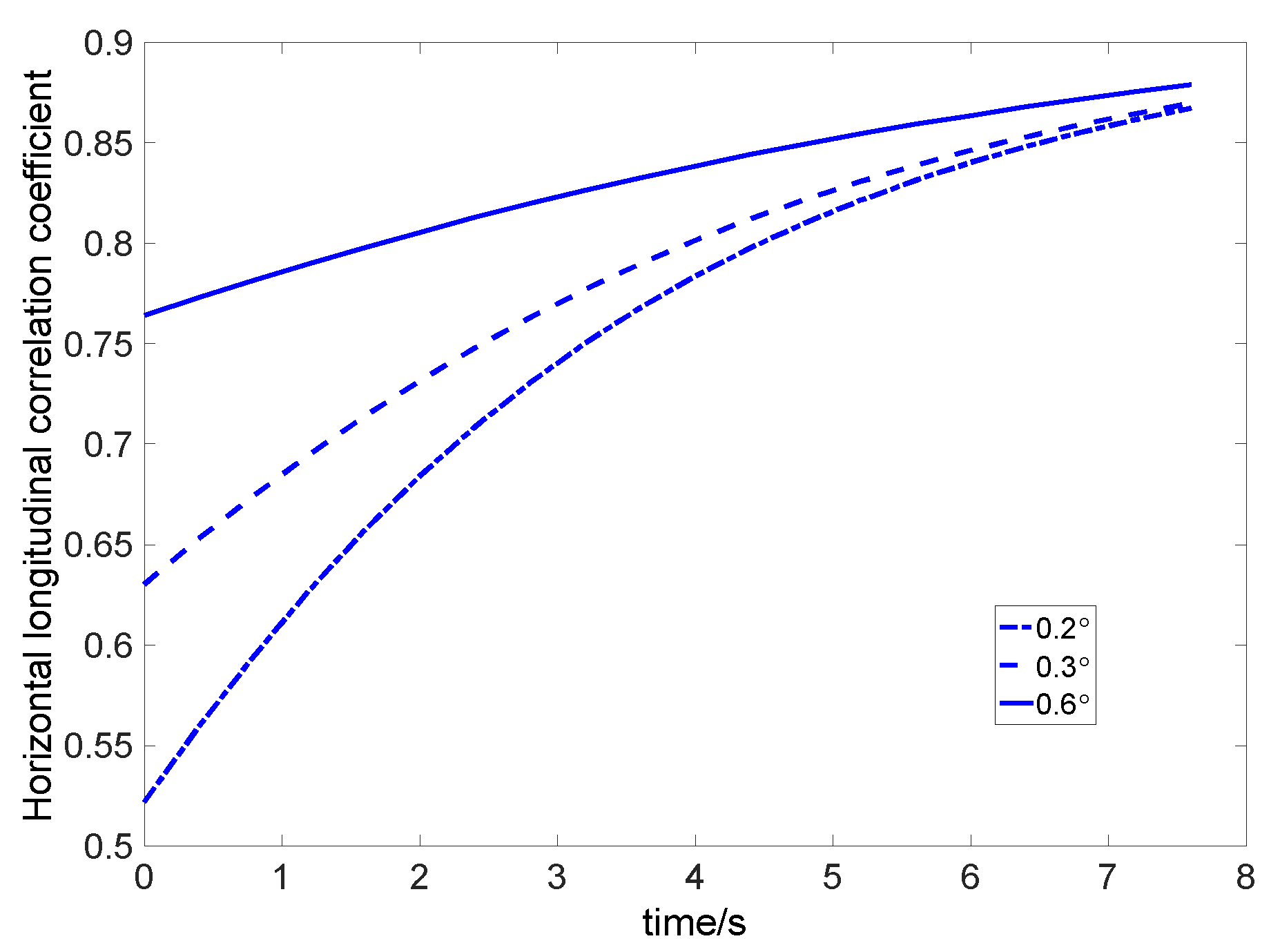
In order to further compare the variation law of horizontal correlation characteristics of remote seabed reverberation under different seabed dip angles, the dip angles of inclined seabed with small dip angles were considered at 0.2° (dotted line), 0.3° (dashed line), and 0.6° (solid line), respectively. The simulated signal frequency was 1500 Hz and the horizontal longitudinal interval was 5 m. The variation of horizontal correlation characteristics is shown in Figure 8. From the comparison results in the figure, it can be found that, under the condition of a gentle slope seabed, the larger the downhill seabed is, the better the spatial correlation characteristics are.

3.2. Experimental Results

In order to verify the correctness of the method proposed, the sea experiments were carried out and the experimental data were obtained. In this paper, the couple mode reverberation model was used, and the backscattering from the rough boundary was considered as one of the main sources for the long-range bottom reverberation. Thus, the scattered field received by hydrophones was considered as the interaction of the incident modes with rough surfaces. The first part of Equation (1) denotes the incoherent parts of the bottom reverberation, which is contributed by diagonal elements of the scattering matrix. The off-diagonal term is presented by the second part of Equation (2). The scattering matrix was thus derived by the coupled mode method, and the detailed derivation can be found in “Journal of Computational Acoustics, Vol. 25, No. 2 (2017) 1750017 (12 pages)” [26]. The simulated curves in the paper were all the averaged incoherent correlation coefficients, and corresponding Equation (13) also considered the process of the nth incident mode and the nth scattering mode. The experiment data were averaged by time widow. The fluctuating part of the data, which was determined by the off-diagonal elements of the coupling matrix, was found to be smoothing well. This is a kind of common proceeding for reverberation data processing [22,27].

The experiment was performed in a seawater waveguide with a half-infinite seabed in an area of the South Sea, China. The depth was about 85 m. The sound speed profile (SSP) was obtained by conductance, temperature, depth (CTD) sensor in water and is shown in Figure 9. There was an obvious thermocline in the range of 20–40 m, which was a typical shallow-water sound velocity distribution gradient. The receiving data were collected using an explosive source with 100-g trinitrotoluene (TNT) charges. The depth of the explosion was 20 m, and the signal was received at a depth of 5 m by a 32-element horizontal array. The element spacing was 1.5 m and the sampling frequency for each hydrophone was 12,000 Hz. According to the nautical chart, the seabed is approximately flat. The seabed sound speed and seabed density had been obtained by inversion method before, at 1775 m/s and 1992 kg/m³, respectively. The experimental results verify the theoretical prediction results of the horizontal longitudinal correlation characteristics of low-frequency ocean reverberation.

Figure 10 and Figure 11 show the data processing and theoretical simulation results of the reverberation experiment. The time series shown in Figure 10 are all narrowband filtered, and such three channel data are chosen is because that we want to display the relationship between the horizontal cross correlation coefficients with the spacing of the hydrophones. As shown in Figure 11, the cross correlation coefficients of 1.5 m spacing are obtained by the data of channel 18 and 19, and the cross correlation coefficients of 3 m spacing are obtained by the data of channel 18 and 20.

During the data processing, 9 valid channels 18–26 were obtained. Figure 10 shows the reverberation time-domain waveforms of channel 18, 19 and 20 after narrowband filtering. Figure 11 is the longitudinal correlation characteristic curve of 700 Hz ocean reverberation when the element spacing is 1.5 m and 3 m. The dotted line with square icon is the result of the measured data processing when the element spacing is 1.5 m, and the dashed line is the theoretical simulation result. The circle graph shows the longitudinal correlation characteristic curve of the measured data when the distance is 3 m, and the solid line is the corresponding theoretical simulation result. The red boxes in the caption are illustrated the chosen time series to evaluate the cross correlation operation. The time windows pointed by the red boxes in channels 18–20 are displayed in Figure 11. The start of the red boxes is the time point of zero in Figure 11

In Figure 11, the following two conclusions can be drawn: (1) when the frequency is constant, the longitudinal correlation of reverberation decreases with the increase of spacing; (2) the longitudinal correlation of ocean reverberation increases with time.

Figure 12 shows the change of the longitudinal correlation characteristics with frequency and time after determining the array spacing. Figure 12 is the measured data of the 600 Hz, 700 Hz, and 800 Hz longitudinal correlation characteristic curve of the real line plus the fork, diamond, and circular icon. The dotted point line and the dotted line are the theoretical simulated longitudinal correlation characteristic curve values of the above three frequencies. It can be seen from Figure 12 that: (1) in the frequency range involved in this paper, the longitudinal correlation characteristics of ocean reverberation decrease with the increase of frequency; (2) in the frequency range involved in this paper, the longitudinal correlation of ocean reverberation increases with the increase of time.

Figure 13 further verifies the frequency characteristics of the marine reverberation longitudinal correlation characteristics. In the figure, the blue solid line with crosses represents the measured data at 200 Hz, and the red solid line is the corresponding longitudinal correlation characteristics of reverberation obtained by the theoretical simulation. The blue dotted line with circles represents the measured longitudinal correlation characteristic curve at 700 Hz, and the red dotted line represents the theoretical simulation results.

In order to further study the horizontal longitudinal spatial distribution characteristics of low-frequency reverberation in the ocean, the cross-correlation processing of reverberation signals from 18 to 26 channels was carried out. Figure 14 shows the spatial distribution of the low-frequency reverberation with the change of array element spacing after the reverberation signal was filtered by a third-octave narrow-band filter with a center frequency of 200 Hz. The horizontal axis is the wavelength ratio of the element spacing, and the longitudinal axis is the longitudinal correlation coefficient. The experimental data processing results are shown as the blue solid line with rhombic markers, and the theoretical simulation results are shown as the red solid line with circular markers. The correlation coefficient between the theoretical simulation characteristic curve and the measured longitudinal correlation characteristic curve was greater than 90%. After calculation, the correlation coefficient was 0.9404.

Figure 15 shows the spatial distribution of low-frequency reverberation with the change of array element spacing after the reverberation signal was filtered by a third-octave narrow-band filter with a center frequency of 500 Hz. Similarly, the horizontal axis is the wavelength ratio of the array element spacing, and the vertical axis is the longitudinal correlation coefficient. The results of experimental data processing are shown as the blue solid line with diamond mark, and the theoretical simulation results are shown as the red solid line with circular mark. The correlation coefficient between the theoretical simulation characteristic curve and the measured longitudinal correlation characteristic curve was greater than 90%. After calculation, the correlation coefficient was 0.9102.

Similarly, Figure 16 and Figure 17 show the variation of the longitudinal correlation characteristic curve of marine reverberation with the element spacing when the central frequencies were 800 Hz and 1 kHz, respectively. The blue solid line with diamond marks is the measured data result, and the red solid line with circular marks is the theoretical simulation prediction result. As shown in the figure, the correlation coefficient between the theoretical prediction results and the measured curve was greater than 90%. After calculation, the correlation coefficients were 0.9851 and 0.9630, respectively.

4. Discussion

The experimental data in Section 3 verify the accuracy of the longitudinal correlation characteristic model of remote seabed reverberation proposed in this paper. In this section, we analyze the influence mechanism of terrain change on the longitudinal correlation characteristics of remote reverberation. It can be seen from the normal wave theory that the sound field is composed of many order normal modes. These normal waves can be decomposed into upward and downward plane waves. The lower the number of modes is, the smaller the grazing angle between the decomposed downward plane wave and the seabed boundary is. In the process of propagation, the energy of large-grazing-angle modes gradually disappears, and the low-order modes with a small grazing angle can propagate far away. In the horizontal shallow-water waveguide, when the sea depth is constant, these up and down waves propagate at a fixed grazing angle. In this process, they interfere with each other to form a stable interference pattern, as shown in Figure 18a. Transmission loss (TL) represents the attenuation of sound in the process of water transmission, and the unit is dB.

In the downhill waveguide environment, the plane wave of each mode originally propagated with a fixed grazing angle further decreases in the propagation process because of the downhill seabed, which causes the change of the temporal and spatial distribution of the sound field, as shown in Figure 18b. Compared with the horizontal seabed, the correlation scale of the sound field interference pattern becomes larger. Therefore, the horizontal correlation coefficient of remote seafloor reverberation in the downhill seafloor waveguide is larger.

In addition to the analysis of the physical mechanism, the following further shows the slow change of the grazing angle of each mode caused by this downhill submarine waveguide from the perspective of data operation. The parameters were as follows: The frequency of the signal was 200 Hz. The sound velocity in water was 1500 m/s, the sound velocity in the liquid semi-infinite seabed was 1800 m/s, and the seabed had an inclination angle of 0.6°.

Table 1. Grazing angles of the first eight modes at the depths of 52.4 m and 63.8 m, respectively.

Modal Number	52.4 m Glancing Angle (°)	63.8 m Glancing Angle (°)
1	3.794	3.205
2	7.624	6.429
3	11.518	9.692
4	15.500	13.005
5	19.589	16.383
6	23.803	19.835
7	28.159	23.376
8	32.642	27.016

shows the changes in the grazing angles of the first eight modes at the seabed at depths of 52.4 m and 63.8 m, respectively. It can be found that, consistent with the previous analysis, the grazing angle of the same order mode decreased with the increase of depth in the downhill seabed.

When the water depths were 52.4 m and 63.8 m, the eigenvalues of the first three-order normal waves were calculated and are shown in Figure 19a. The eigenvalues of the first four-order normal waves at depths of 63.8 m and 136.3 m, respectively, are shown in Figure 19b. It can be found that, in addition to the trend of gradual change to the lower-order modes, the eigenvalue difference between the different modes $\Delta {\xi }_{mn}={\xi }_m-{\xi }_n$ in the downhill seabed became smaller and smaller with the increase of depth. In the sound field, the interference scales $l$ and $\Delta {\xi }_{mn}$ were inversely proportional [28], so the correlation scale of the interference pattern in Figure 18b increased with the increase of depth. In other words, with the increase of the depth of the downhill seabed, there is a more stable, large-scale interference structure. Compared with the horizontal seabed topography, the change of the interference structure with the topography is the main reason for the enhancement of the horizontal longitudinal correlation in the downhill seabed topography. According to the couple mode reverberation model, the scattered field received by hydrophones is considered as the interaction of the incident modes with rough surfaces. By this view, the reverberation field is evaluated as the first-order perturbation of the propagation field. Hence, the long-range reverberation coherent property is affected seriously by the characteristic of the waveguide [24]. For the case of a wedged waveguide, we calculated the eigenvalue, and the results showed that the coherent structure of the propagation field was influenced by the depth of waveguide. Considering the linear acoustics theory, the bottom reverberation and the first-order perturbation of the field would also have similar phenomenon.

It should be pointed out that Figure 14, Figure 15, Figure 16 and Figure 17 show the variation law of horizontal longitudinal correlation characteristics of 200 Hz, 500 Hz, 800 Hz, and 1 kHz, respectively, with array element spacing. In order to unify the dimension, the horizontal axis coordinate was (d/λ). The overall trend of the longitudinal correlation coefficient of the three groups of graphs is consistent with the measured data. The similarity of the two was determined as 0.9404, 0.9102, 0.9851, and 0.9630, respectively. The results show that, with the increase of the array spacing, there is a certain deviation between the simulation results and the measured results, which is due to the uncertainty of the seabed scattering description. For seafloor reverberation, especially in low- and medium-frequency bands, the scattering mechanism is complex, including the scattering from the rough undulating interface and the scattering from the uneven bottom material. The theoretical model in this paper is a calculation and analysis of the average trend of reverberation as the longitudinal correlation characteristics. The characterization of uncertainty and randomness of seafloor scattering is not given in this model.

5. Conclusions

On the basis of the coupled normal mode reverberation model, this paper systematically studies the temporal/spatial/frequency variation of the horizontal longitudinal correlation characteristics of long-range reverberation. The approximate relation of spatial correlation of reverberation with time, space, and frequency is given quantitatively. The influence of the waveguide boundary on the spatial and temporal distribution of long-range seabed reverberation is discussed, and the physical mechanism of the influence is analyzed from the perspective of the mode change caused by the waveguide boundary. The results show that the horizontal longitudinal correlation characteristics of long-range seabed reverberation decrease with the increase of frequency, increase with the increase of reverberation time, and decrease with the increase of array spacing. For the case of a gently varying seabed with a small angle of inclination, the longitudinal correlation characteristics of long-range seabed reverberation are enhanced. However, it is still necessary to point out that the theoretical model of this paper approximates the longitudinal correlation characteristics of the remote reverberation level, and gives a prediction of the overall trend of the longitudinal correlation characteristics of the reverberation level. The diversity and inhomogeneity of seafloor scattering and the influence of water fluctuation on long-range reverberation leads to a deviation between the measured data and the theoretical prediction results. The comparison results in this paper also illustrate this point; that is, the overall trend of horizontal longitudinal correlation characteristics of remote reverberation is consistent with the edicted results of the model and the measured data.