Article

Evaluation of Groundwater in the Coastal Portion of Guasave, Sinaloa for White Shrimp Farming (Penaeus vannamei) through VES, Chemical Composition, and Survival Tests

by
Mauro Espinoza Ortiz
1,
Juan Pablo Apún Molina
2,*,
Héctor José Peinado Guevara
3,*,
Jaime Herrera Barrientos
4,*,
Salvador Isidro Belmonte Jiménez
5,
María de los Ángeles Ladrón de Guevara Torres
5 and
Omar Delgado Rodríguez
6
1
Instituto Politécnico Nacional, CIIDIR Unidad Sinaloa, Programa de Doctorado en Red en Ciencias en Conservación del Patrimonio Paisajístico, Guasave C.P. 81100, Sinaloa, Mexico
2
Instituto Politécnico Nacional, CIIDIR Unidad Sinaloa, Guasave C.P. 81100, Sinaloa, Mexico
3
Escuela de Ciencias Económicas y Administrativas, Universidad Autónoma de Sinaloa, Guasave C.P. 81100, Sinaloa, Mexico
4
Centro de Investigación Científica y de Educación Superior de Ensenada, Baja California (CICESE), Ensenada C.P. 22860, Baja California, Mexico
5
Instituto Politécnico Nacional, CIIDIR Unidad Oaxaca, Santa Cruz Xoxocotlán, Oaxaca C.P. 71230, Oaxaca, Mexico
6
División de Geociencias Aplicadas, Instituto Potosino de Investigación Científica y Tecnológica (IPICyT), San Luis Potosi C.P. 78216, San Luis Potosí, Mexico
*
Authors to whom correspondence should be addressed.
J. Mar. Sci. Eng. 2021, 9(3), 276; https://doi.org/10.3390/jmse9030276
Submission received: 14 January 2021 / Revised: 23 February 2021 / Accepted: 25 February 2021 / Published: 4 March 2021
(This article belongs to the Special Issue Coastal Engineering: Sustainability and New Technologies)

Abstract

:
We studied the potential of white shrimp farming with groundwater from the coastal aquifer of Guasave, Sinaloa. The use of water from the aquifer in aquaculture represents challenges due to variability in the quality of groundwater. We did twenty-three vertical electrical soundings (VES), performed to guide the search for continental groundwater, obtaining the resistivity of the saturated formation (Ro) and a relationship with resistivity of aquifer water (Rw) = 0.4478 Ro + 0.8371. We obtained ionic content and nutrients from shrimp farming water. Also, a positive correlation was found between the electrical conductivity of the aquifer water (inverse of Rw) with chlorine, sodium, magnesium, and calcium ions in 34 water samples. The analysis of ions and ammonia-nitrogen, nitrates, phosphates, potassium, manganese, and calcium were used to select suitable sites to perform in two shorts bioassays: natural aquifer water and adding KCl and Mg2Cl to simulate diluted seawater. In most natural waters, survival of larvae was higher than 60%, and in simulated seawater survival improved only in two sites. Building the Rw-Ro relation allowed us to infer the quality and suitability of water and the positioning of the most suitable place for drilling. Finally, Rw relation with dissolved ions allowed us to estimate aquifer water quality and reduce uncertainty.

1. Introduction

Aquaculture is a primary sector activity with high growth potential. This, in addition to being a food source of great nutritional value, has provided socioeconomic benefits [1]. Mexico is one of the largest aquaculture producing countries in Latin America and the Caribbean [2]. The main species considered as targets are snapper, mollusk, white shrimp, and tilapia [3].
Aquaculture is a source of jobs in Sinaloa. It contributes to food security and poverty alleviation [4]. Shrimp farming in continental waters is a viable alternative for the development of small and medium producers in rural communities [5].
The quality of the water that supplies a crop is one of the predominant factors in aquaculture. In Mexico, the water sources for aquaculture developments come to a greater extent from lagoons, rivers and the sea [6]. Recent research shows the potential for the development of systems for aquaculture organisms using groundwater in tilapia [7] and white shrimp [5,8], obtaining considerable productive returns. So, groundwater is a viable alternative for continental aquaculture [9], and according to Valenzuela et al. [10] and Valenzuela et al. [8] the ionic composition of groundwater is more important in shrimp farming at low salinities.
Extensive aquaculture farms show a gradual tendency to promote configurations for more intensive production [11]. This due to the pathologies observed in shrimp farming.
In the production processes with groundwater it is fundamental to preserve its quality and quantity, so it is a priority to determine the appropriate places for its use in aquaculture [12,13], as well as its availability and quality so that the physicochemical parameters are in optimal ranges for the growth of aquatic organisms prior to the construction of an aquaculture farm [14].
To directly evaluate the water characteristics of an aquifer is a costly process, since it requires drilling that makes large-scale evaluation impossible [15]. Given this, the use of indirect methods (VES) in conjunction with direct information is an alternative to characterize the water quality of an aquifer. This is achieved through the study of the electrical properties of the water of the aquifer formation using vertical electrical sounding (VES) [16,17,18,19,20,21]. This is a method of geophysical prospection by direct current [22] which allows knowing the electrical resistivity of the Ro aquifer formation [23]. On the other hand, Peinado et al. [24] has characterized the water quality of an aquifer by establishing relations between the electrical resistivity of the water (Rw) and electrical resistivity of the aquifer formation (Ro). It is proposed here to find the Rw–Ro relation for the study area, as well as the relation between Rw and the concentration of groundwater ions necessary for the survival of shrimp. So, once the aforementioned relations have been established, in a place in the study area where there is no drilling through the Ro value obtained by VES, the quality of the groundwater for shrimp farming can be inferred.

2. Materials and Methods

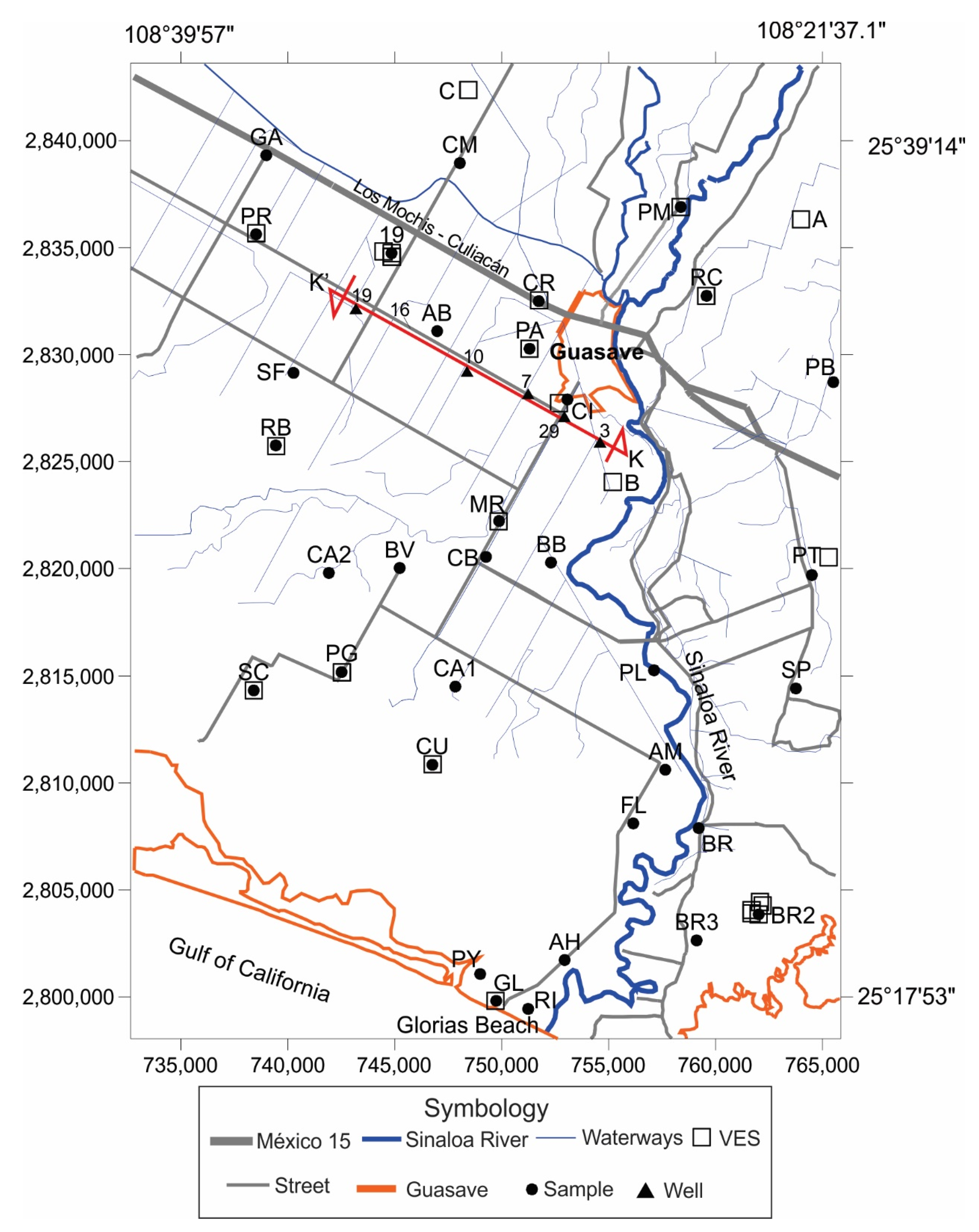
2.1. Description of Study Area

The study area is within the aquifer of the Río Sinaloa. It is located at coordinates 25° 16′ 30.9″ to 25° 41′ 31.5″ north latitude and from 108° 21′ 35.9″ to 108° 40′ 54″ west longitude (Figure 1). Based on studies carried out of geological, geophysical, and hydrogeological evidence, the Río Sinaloa aquifer has been defined as of free type, heterogeneous, and anisotropic, with alluvial and fluvial sediments of varied granulometry. The thickness of the sediments in the central portion of the coastal plain in Guasave, Sinaloa is of several hundred meters [25].
The climate is dry, warm, and very hot. For the period of 1986 to 2016, the average annual temperature is 24 °C [26]. Average annual rainfall is 429.2 mm. There are rains in two periods, one in summer with abundant rainfall from July to October and another in winter with rains from November to January with precipitation less than 5% of the annual average [25].
The aquifer structure in terms of aquifer material availability, boundaries, and geometry is determined by correlating six lithologic columns of wells (3, 29, 7, 10, 16, and 19) with depths ranging from 120 m to 150 m, provided by the National Water Comission(profile K-K’, Figure 2).

2.2. Groundwater Sampling

In the study area, water samples were collected in 34 wells (Figure 1); 28 of them were active and six were drilled for the extraction of water samples. The samples were labeled and stored in 1 L plastic bottles. At the moment of the extraction, the depth of the water table was measured with a tape. Regarding pH, electrical conductivity (EC), Total Dissolved Solids (TDS), and temperature, the measurement was carried out with a Hanna HI98130 equipment. The content of the NH4+ samples was measured with a portable photometer brand YSI 9500. Each sampling point was georeferenced with a GPS Garmin eTrex brand.
Wells are designated with acronyms that refer to the place where they are located: AB, AH, AM, BB, BR, BR2, BR3, BV, CA1, CA2, CB, CI, CM, CR, CU, FL, GA, GL, MR, PA, PB, PG, PL, PM, PR, PT, PY, RB, RC, RI, SC, SF, SP y 19.
The samples were placed on ice and transported to the Interdisciplinary Research Center for Integral Regional Development Sinaloa Unit (CIIDIR Sinaloa) fish aquaculture laboratory, Sinaloa, where the presence of nutrients (NO3, NO2, K+, NH4+, PO43−) was determined through colorimetric techniques using a YSI 9500 photometer (Yellow Springs, OH, USA). Metals Mn and Fe were determined using a HANNA 82,300 photometer (Hanna Instruments, Limena, Italy). Table 1 indicates the method to measure each parameter, as well as the range, wavelength, accuracy, and resolution of these instruments.
To measure the concentration of the parameters, 10 mL volume glass cuvettes were used for each sample following Table 1. Samples that exceeded the measurement concentration range of the spectrophotometer were diluted.
The ionic composition (Na+, Cl, Ca+2) of the samples was determined in a laboratory of the 075 Irrigation District belonging to the National Water Comission (CNA).

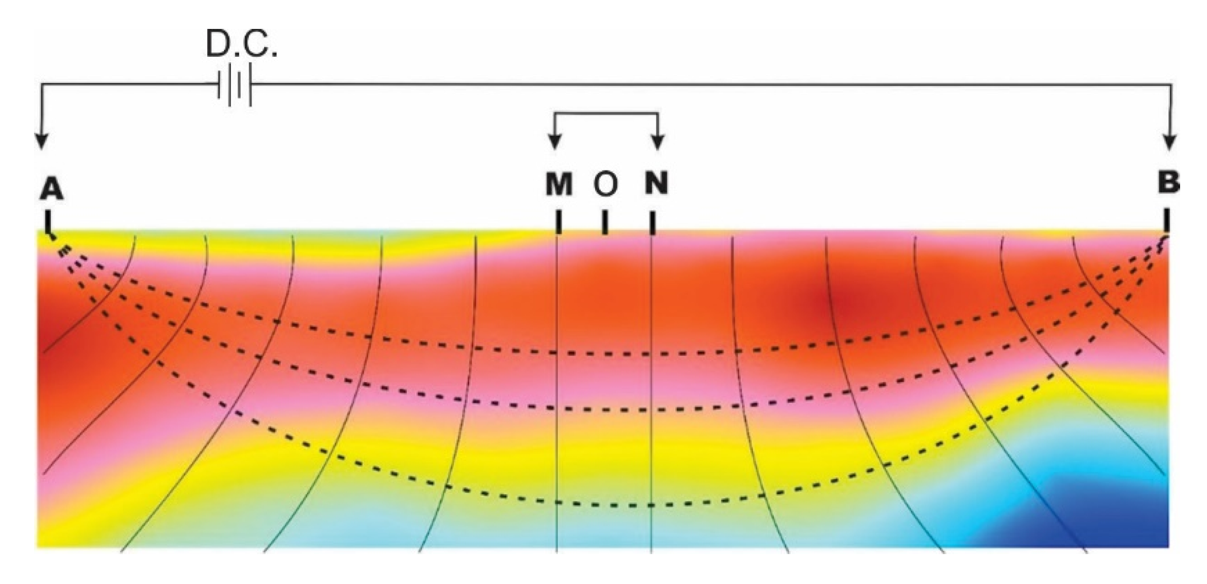
2.3. Vertical Electrical Soundings

To carry out the vertical electrical soundings (VES) a tetraelectrodic device was used in its Schlumberger mode (Figure 3). The center of symmetry of the device is O so that the distances OA = OB = L y OM= ON = a, in addition, it maintains the relation:
MN ≤ (AB/5),
A continuous electric current of intensity I is injected through electrodes A and B, which will create an electric field in the subsoil. This field produces a potential difference ∆V between the electrodes M and N. Then, with these measurements, the apparent resistivity of the ground is obtained:
ρa = K ∆V/I,
where
K = π L^2/a,
Keeping the center of the device at O and with the purpose that the injected electric current penetrate the subsoil deeper, the separation between the electrodes is gradually increased, taking care that the relation given by equation 1 is fulfilled, thus obtaining the value of ρa as a function of each of the AB/2, separations, obtaining the apparent resistivity curve of the subsoil (AB/2 vs ρa). From this, by direct modeling considering that the terrain is formed by horizontal homogeneous and isotropic layers, the electrical resistivity of the aquifer formation, Ro, is obtained.
The number of VES were 23, each one was georeferenced in Universal Transverse Mercator coordinates (UTM). AB/2 separations of: 5, 10, 20, 30, 40, 50, 60, 80, and 100 m were used. Of the VES carried out, 13 were made at sites where there are wells and groundwater EC measurements. VES were modeled with the software RESIXP. The product of the modeling, the saturated thickness and the electrical resistivity of the aquifer formation (Ro) were obtained.
This was related to the electrical resistivity of the water (Rw) in the aquifer. The latter was obtained from the following expression:
Rw = 10/EC,
where EC is the electrical conductivity of the aquifer water in mS/cm.

2.4. Selection of Sites for Aquaculture Farming

Table 2 was prepared from a bibliographic review. It contains the range of variation, maximum values and concentrations of various physical and chemical parameters of groundwater for shrimp farming. Considering the values of these parameters, water samples from wells that met these values were selected.
The parameters are: electrical conductivity (EC), pH, total dissolved solids, ionic composition (Na+, Mg+2, Ca+2, Cl), heavy metals present (Mn, Fe) and nutrients (NO3, NO2, K+, NH4+, PO43−).

2.5. Forty Eight Hours Survival Evaluation Test of P. vannamei Test

With the purpose of evaluating the survival of shrimp culture in groundwater, 70 L of groundwater were collected from each of the following seven sites: GL, CU, RB, SC, PA, PR and La 19. The samples were transported to the Department of Aquaculture of CIIDIR, Sinaloa and there they were kept in aeration with diffuser stones from the beginning of the cultures until the end of the same. The shrimp larvae culture was developed over a 48 h period in two phases: (a) with direct transfer; and (b) with direct transfer adding KCl and Mg2Cl to the water, in a similar way to that proposed by Valencia et al. [5].

2.5.1. Forty Eight Hours Survival with Groundwater

Groups of 10 postlarvae (initial weight 20.48 ± 2.08 mg) gradually acclimatized at a rate of (2 g/L/h) until a salinity of 4 g/L were transferred to containers with 2 L of water from each well for 48 h. At the end of this period, a count was made and a survival rate greater than or equal to 60% was considered as a criterion to select water samples from the wells for possible field cultivation.
As control treatments: C1 sea water was used at 30 g/L and C2 sea water diluted at 4 g/L. The cultures were performed in triplicate and fed twice a day (09:00 a.m. and 17:00 p.m.) ad libitum.

2.5.2. Forty Eight Hours Survival with Addition of Salts to Groundwater

Groups of 10 postlarvae (30.42 ± 2.42 mg) acclimated to 4 g/L were transferred to containers with 2 L of water from each well. The water samples where short-term survival (48 h) was ≥ 60% were selected.
As control treatments: C1 sea water was used at 30 g/L and C2 sea water diluted at 4 g/L. For the addition of salts in each well, the concentration of potassium chloride and magnesium chloride was calculated following the equation proposed by Boyd and Thunjai [31].
It was supplemented with potassium and magnesium salts using potassium chloride (KCl 99.0% Faga Lab®, Mocorito, Sinaloa, Mexico) and magnesium chloride (MgCl2 99.0% Faga Lab®, Mexico) for cultivation at theoretical salinity according to Boyd and Thunjai [31]. The cultures were performed in triplicate and fed twice a day (09:00 a.m. and 17:00 p.m.) ad libitum.

2.6. Statistic Analysis

The survival percentage of the bioassays were transformed with arcsine√p [5,32] due to the lack of normality of the percentages from 0 to 100% with binomial distribution [33]. A one-way analysis of variance (ANOVA) (p < 0.05) and a Tukey test (p < 0.05) was performed to identify differences between groups.

3. Results

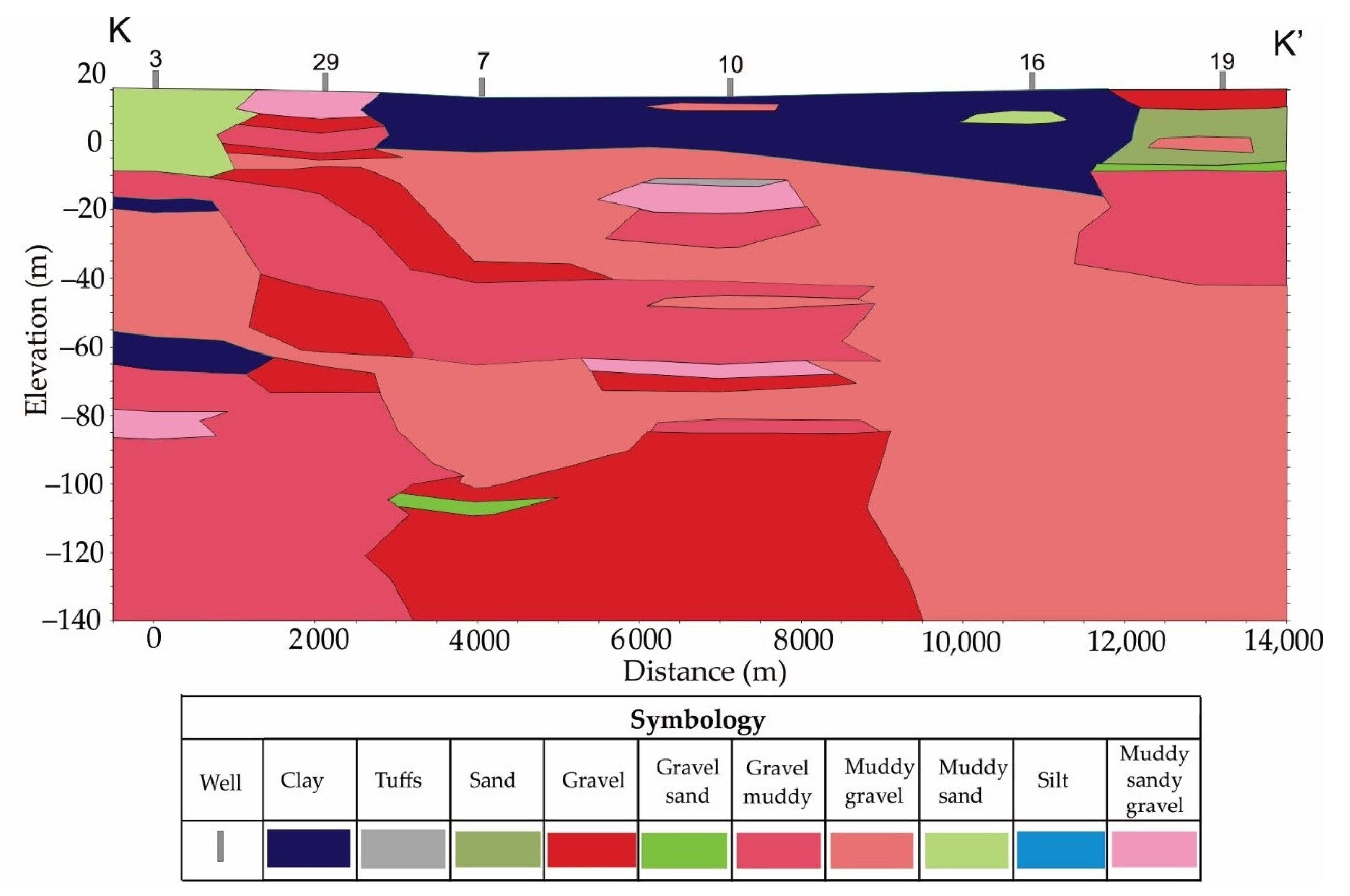
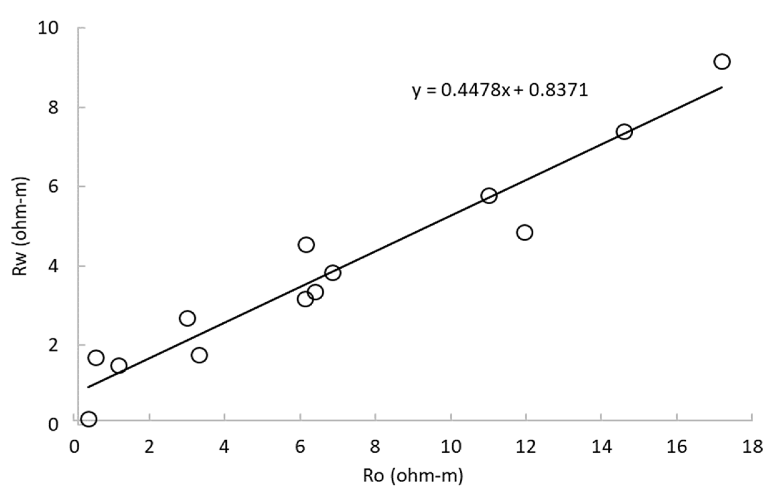
3.1. Aquifer Structure, Rw and Ro Relation

Table 3 shows 13 wells with their coordinates, static level depth (SL), electrical conductivity (EC) of the water in the well, resistivity of the aquifer formation (Ro), and resistivity of the aquifer water (Rw). VES was performed in each well and, from the apparent resistivity curve obtained and interpreted with the program RESIXP, the value of Ro indicated in Table 3 was obtained. With the Ro and Rw values, a linear regression analysis was performed resulting in a correlation coefficient of 0.933 (Figure 4). The equation that describes the relation between Ro and Rw is: Rw = 0.447Ro + 0.8371. That is, the higher the resistivity of the saturated formation, the higher the resistivity of the aquifer water.
The structure of the aquifer was determined by the lithologic sequences of wells 3, 29, 7, 10, 16, and 19 (Figure 2). The lithologic column of these six wells was used to construct the section of the aquifer environment corresponding to the K-K’ profile (Figure 1). The columns were topographically located and correlated, showing that the aquifer environment behaves as free in wells 3, 29, and 19 and as confined in wells 7 and 16. The distribution of the aquifer materials is mainly due to the eolian and fluvial deposits of the Sinaloa River. These detrital sediments were transported and deposited by the migratory dynamics of the Sinaloa River, arranged so that coarse materials such as gravels were deposited in the deeper portions and fine materials in the shallower part. This is due to variations in the historical intensity of the flow velocity.
The coarse materials are characterized by a high hydraulic transmissivity. On the other hand, the lithological columns in this section did not penetrate the geological and hydrogeological basement, which indicates that the wells partially penetrate the aquifer.
Regarding the upper and lower limits of the aquifer, the upper limit (between wells 3, 29, and 19) is the atmospheric pressure and the pressure of an impermeable medium (between wells 7, 10 and 16). As a lower boundary, the aforementioned wells did not cut impermeable medium.

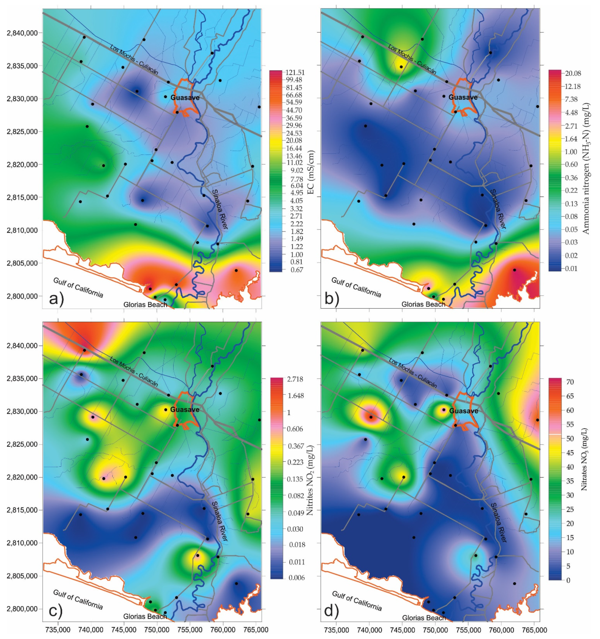
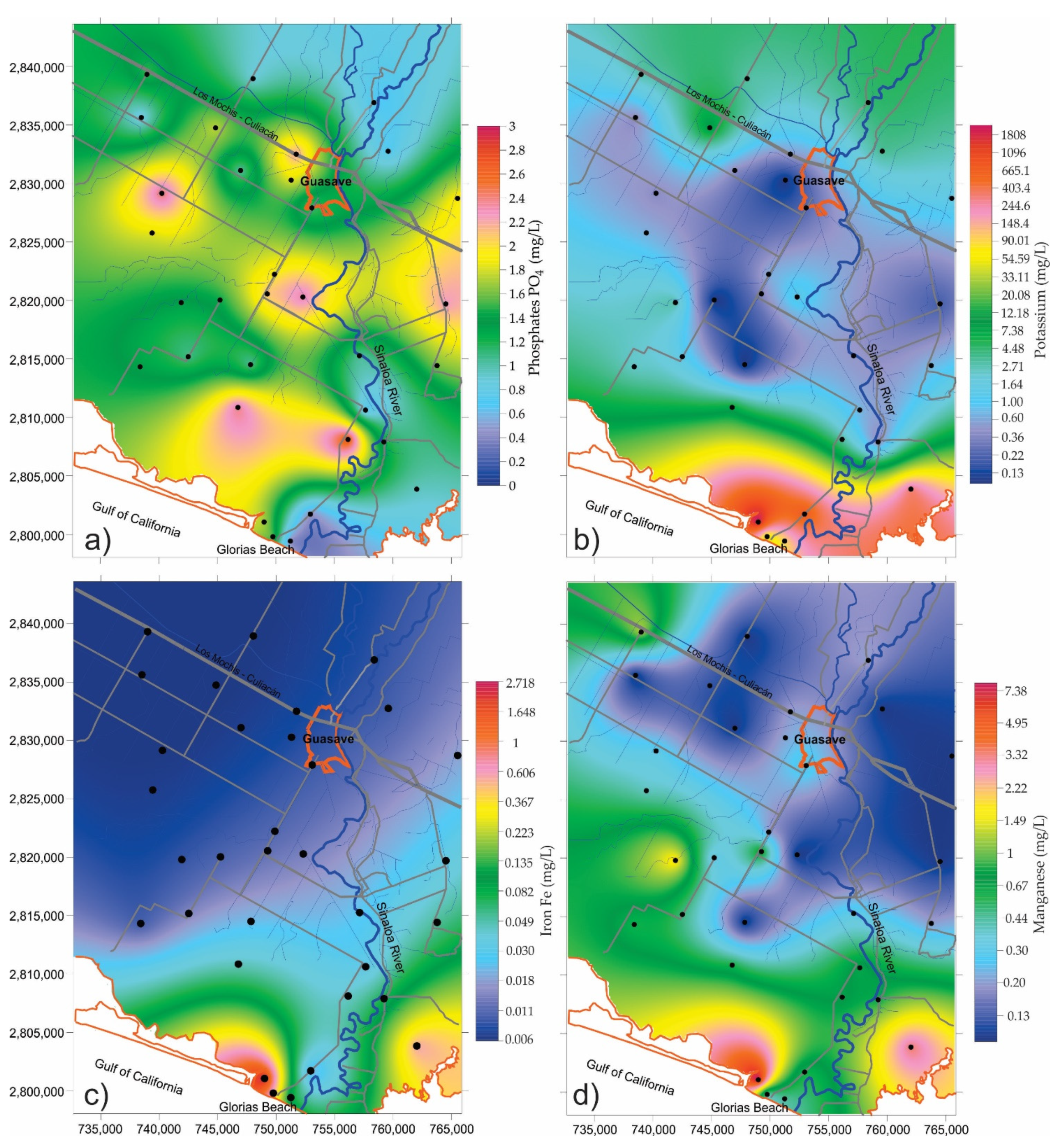
3.2. Analysis of Collected Groundwater Samples

It was indicated the behavior of the physical-chemical parameters whose values are included in the intervals of Table 2. The static level depth average of 34 water samples was about 2.98 ± 1.85 m under natural terrain and the bottom of the well was not greater than 15 m in all wells analyzed in the present study.
The pH of the water extracted from the wells was measured in situ. This showed an average of 8.02 ± 0.32 with a maximum value of 8.83 at the La 19 site and a minimum of 7.48 at the Las Glorias (GL) site. In areas outside the city, there were areas registered with groundwater with a neutral trend.
The behavior of the electrical conductivity of the groundwater predominated as saline in the coastal zone and in the localities near the municipal seat. The average was 11.06 mS/cm and the maximum values were in El Pitahayal (PY), AH, and La Brecha 2 (BR2) with 128.4 mS/cm, 95 mS/cm, and 61 mS/cm, respectively. Figure 5 (upper left) shows the variation in electrical conductivity, higher on the coastline, decreasing as it moves towards the continent.
The ammonia nitrogen concentration (see Figure 5, upper right) at the BV, CA2, PT, BR, CB, BB, MR, and PA sites was zero with the equipment YSI 9500, which has a minimum detection resolution of 0.01 mg/L, these values are mainly found in communities near the municipal seat. In contrast to this value, the La Brecha 2 (BR2) site stands out, which had the maximum concentration of 28 mg/L. The behavior of ammonia nitrogen can be observed in Figure 5, with a predominant central strip of low value, flanked to the north and south by higher levels.
Nitrites increase from south to north with lateral variations (Figure 5, lower left). The 34 samples in this study showed a mean of 0.18 ± 0.46 mg/L with a maximum of 2.68 mg/L at the site El Gallo (GA), near a lined irrigation canal. Only in La Bebelama (BB) site, no concentration was detected with the detection resolution 0.001 mg/L. This variable did not show an increasing trend in the coastal zone.
Nitrates (Figure 5, lower right) increase from south to north. Their average is 16.30 mg/L and they present a variation from 0.31 to 71.86 mg/L. The maximum value was presented in the northeast area at the San Fernando (SF) site, to the northwest in Palos Blancos (PB) with a value of 62.46 mg/L and a minimum value of 0.31 mg/L was presented in El Sacrificio (SC).
The behavior of phosphates in groundwater in the study area is shown in Figure 6, upper left. This presents alternations of maximums without defined behavior. The data showed an average of 1.46 ± 0.62 mg/L with a maximum value of 2.69 mg/L in Las Flores (FL) and 2.44 mg/L in San Fernando (SF). The minimum value was presented in Boca del Rio (RI) with a concentration of 0.41 mg/L.
Potassium (Figure 6, upper right) varies from the coast to the mainland. On the coast it acquires its highest value and in the continent the lowest. Considering the resolution of the measuring equipment, the potassium ion concentration was not detected at four sites (RB, PL, CB, and CI). The other sites presented concentrations in the range of 0.1 to 70 mg/L in the area near the municipal seat. Elevated values of 780 mg/L were found in coastal areas and 2440 mg/L at the HA site.
Figure 6, bottom left and right, shows the variation of iron and manganese, respectively. Both present a variation of high in the south and low in the north. In the case of iron, the low concentration is distributed to the NW and, for Mn, to the NE. The highest and lowest values were found in localities PY and BR2, respectively.

3.3. Correlation Matrix Matrix of Physicochemical Parameters

Table 4 shows the correlation matrix between the parameters measured in groundwater, observing high correlations between the ions of potassium, magnesium, calcium, chlorine, sodium, and some metals such as manganese and iron with electrical conductivity with correlation coefficients of 0.92, 0.99, 0.99, 0.98, 0.99, 0.82, and 0.80 respectively, this indicates that by increasing the electrical conductivity the concentration of these ions or metals increases in this study area. That is, the electrical conductivity of the water is a parameter that is related to parameters that intervene in the survival of shrimp and, in turn, the said conductivity is related to the resistivity of the water in the Ro formation, obtained by means of VES. Hence the importance of VES as a guide in the search for water for shrimp farming.

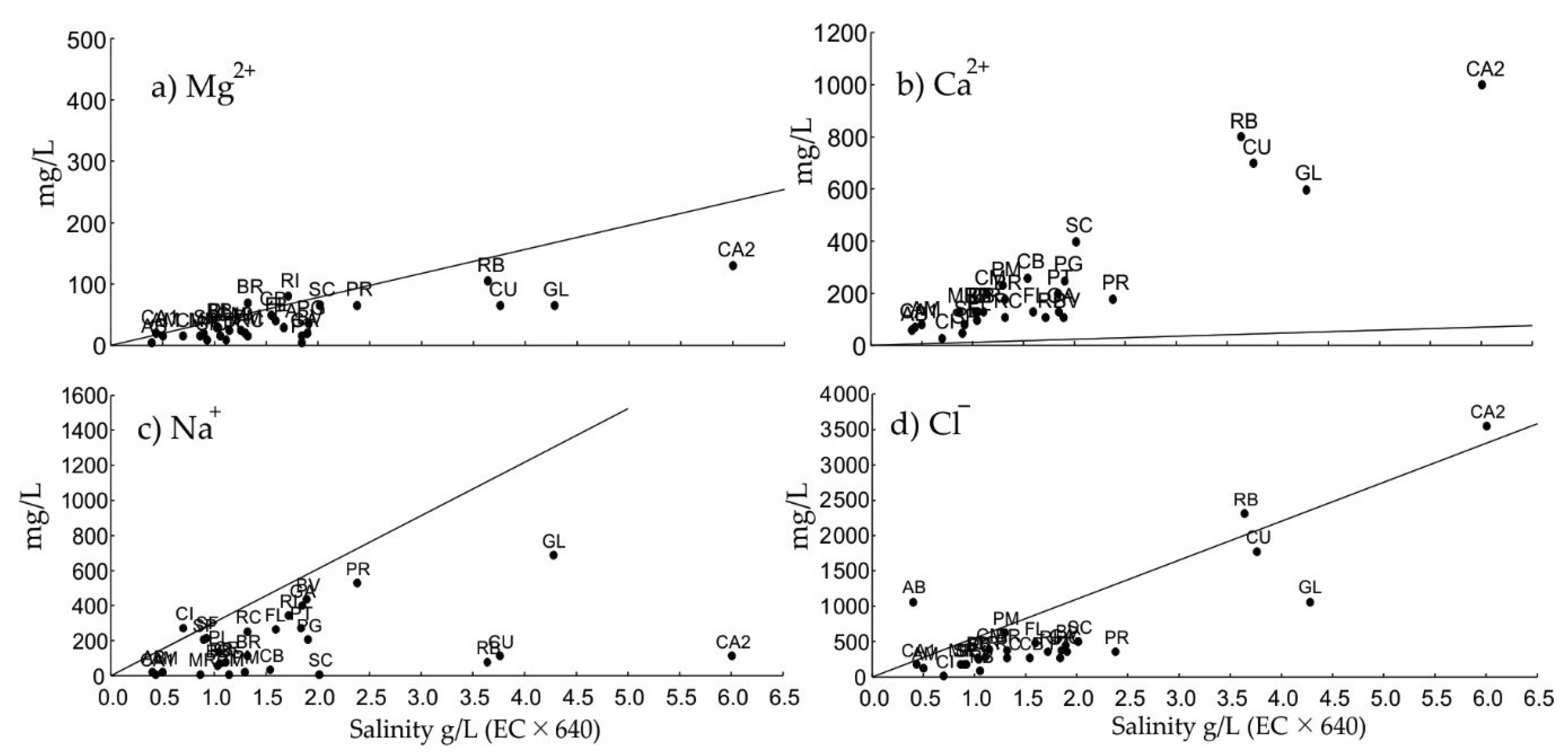
3.4. Ion Concentration Versus Total Salinity of Diluted Seawater
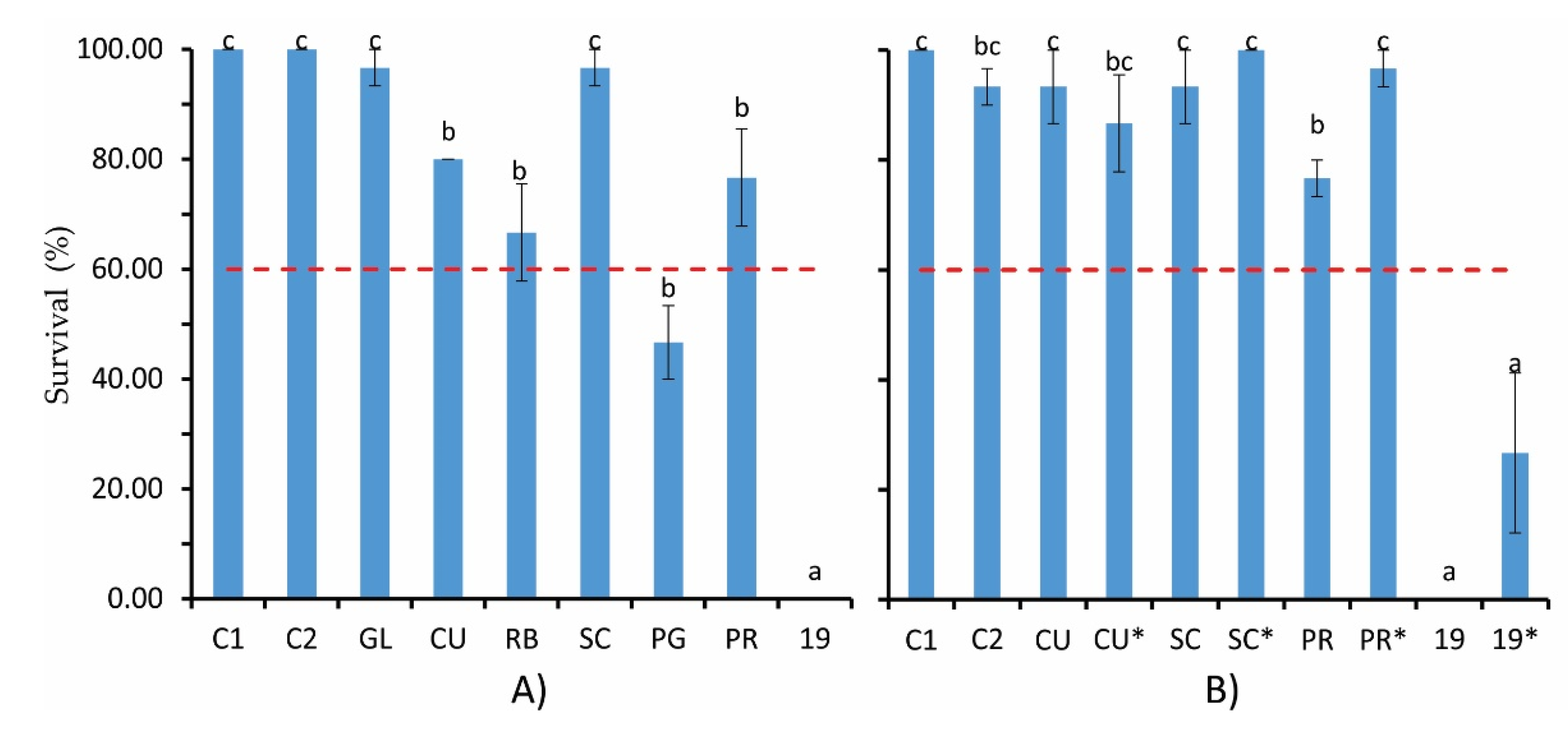
For shrimp farming in low salinity water or, where appropriate, groundwater, Boyd and Thunjai [31] and Roy et al. [34] emphasize that ion concentrations for an adequate shrimp culture should remain in a range equivalent to diluted seawater, however, in this study area, ideal concentrations were not present in some ions such as potassium and magnesium.
Figure 7 shows the behavior of the concentration of magnesium, calcium, sodium, and chlorine ions at sites with salinity between 0 and 6.5 g/L and their respective equivalent concentration of diluted seawater. The calcium ion concentration of the samples was above the theoretical dilute seawater. In the PY locality it reached a maximum of 9000 mg/L with a salinity of 64 g/L and, in CI, a minimum value of 30 mg/L. The sodium concentration generally showed a lower value than the equivalent concentration of diluted seawater, these in a range of 11.5 to 13,800 mg/L. Chlorine presented a minimum concentration of 17.75 mg/L in the CI site and a maximum value of 26,625 mg/L in PY. The magnesium ion maintained values above the equivalent concentration of seawater, with a maximum value in the PY locality of 3600 mg/L and a minimum of 6 mg/L in CI.

3.5. Bioassays

3.5.1. Bioassay 1 (48 h)

Figure 8A shows the result of the survival percentages of the shrimp postlarvae of the bioassay without adding salts. Preliminary 48 h cultures were performed with water from seven locations to observe the survival of the organisms. From the statistical analysis it was observed that there is no significant difference (p < 0.05) between the two controls (C1 and C2) and in the Las Glorias (GL) and El Sacrificio (SC) sites, but a difference was observed with the Las Culebras (CU), Roberto Barrios (RB), Progreso (PG), and Las Parritas (PR) sites. In the 48-h test it was observed that at only in two sites, La 19 (19) and La Progreso (PG), survival was not greater than 60%.
From the results of the first bioassay, four sites (CU, SC, PR, and 19) were taken to perform the second bioassay with the addition of salts of potassium chloride and magnesium chloride at the concentration proposed by Boyd and Thunjai [31] at the respective salinity for a groundwater culture.

3.5.2. Bioassay 2 (Addition of Salts)

Figure 8B shows the results of bioassay 2. Potassium chloride and magnesium chloride were added to the CU, SC, PR, and 19 sites. The first three obtained survival rates greater than 60%, with the exception of site La 19, which had had a survival rate of 0% in bioassay 1. The results did not show significant differences with respect to the controls (C1 and C2) and the study sites, with the exception of the PR site and La 19. Site 19 observed without the addition of salts a survival of 0% and with the addition of salts the survival was 26 ± 14%; that is, the addition of potassium and magnesium ions improved the survival in organisms cultured with La 19 water, however, it was not significant to be selected as a potential site for shrimp culture.
The result observed in the organisms cultured with the Las Parritas water source (significant difference) indicates that it can potentially be used for shrimp cultures, since an increase in survival was observed in the first 48 h. It is important to highlight that it was observed that in the cultures where salts were added as in the control bioassays, that the shrimp showed more activity (less lethargy) and energy, unlike the organisms grown in the bioassays where no salts were added.

4. Discussion

4.1. Variations of EC and Its Relation to Various Ions

In coastal areas, the electrical conductivity (EC) of water varies from moderately saline to saline, according to the Heath [35] classification. This variation is due to the interface of groundwater and seawater. Chidambaram et al. [36] reported similar behavior in a coastal aquifer, commonly influenced by the interaction of groundwater and sea. In this study the groundwater EC ranged from 2.68 mS/cm (RI site) to 95.6 mS/cm (AH site). Similar results have been reported by Peinado et al. [21] who characterized the coastal zone of Guasave in Las Glorias beach with 24 water samples from drillings, finding a variation in the EC that ranges from 1.96 to 88.60 mS/cm.
At the Guasave seat, Sinaloa Peinado et al. [37] found from 66 water samples that the EC varies from 0.18 to 8.08 mS/cm. These values are similar to those obtained in this work, ranging from 0.62 to 9.38 mS/cm.
The correlation of EC with Na+, Mg+2, Ca+2, Cl, Mn, Fe, y K+ (Table 4) is positive and similar to that reported by Shroff et al. [38]. These authors showed good correlation between EC and the variables Cl, Na+, Mg+2 y Ca+2 of the groundwater of an aquifer in India. Other authors have also identified relations between EC and other ions [37,39,40].
Regarding the Ca+2 concentration of groundwater, this turned out to be higher than that of diluted seawater. Boyd and Thunjai [31], as well as Valencia et al. [5], indicate that this is explained by the genesis of the aquifer.
At a couple of sites, the iron concentration is 0.56 mg/L and 2.56 mg/L, not suitable for shrimp farming or human health, since they are higher than the 0.3 mg/L established by NOM-127-SSA1-1994. Saoud et al. [41] and Rodríguez et al. [42] carried out sampling in the municipality of Guasave without reporting iron concentrations higher than 0.3 mg/L.
Near the coastal zone (site BR2) in a well at a depth between 6 and 15 m, ammonia nitrogen was high at 28 mg/L. This is explained by the presence of organic matter. Similarly, Mastrocicco et al. [43] reported elevated concentrations of NH4+ in a coastal aquifer mainly due to the presence of muddy sediments with fine material. Valencia et al. [5] found a maximum concentration of nitrates of 108 mg/L and 2.88 mg/L of nitrites. In this work the maximum values for these two variables were 71.86 mg/L and 2.68 mg/L, respectively.

4.2. Application of Ro–Rw and Rw–Ion Concentration Relationships

The resistivity of the aquifer water Rw and the resistivity of the aquifer medium, Ro (obtained by vertical electrical sounding) are related in a linear way. So that through this relation, Ro–Rw in connection with the strong Person correlations that exists between Rw and the ions Na+, Mg+2, Ca+2, and Cl−1 the aquifer is characterized and the places with groundwater are determined most suitable for growing shrimp P. vannamei.
The relation between Ro–Rw is linear and is given by Rw = 0.449Ro + 0.74 with a correlation coefficient R2 = 0.933. This result is similar to that obtained by Peinado et al. [44] of Rw = 0.427Ro + 1.987.
The Ro–Rw relation under a linear scheme presented a good adjustment like the one found by Archie [45] from data of records in wells, so the Archie relation is applicable in aquifers like the one studied here. The Ro resistivity at the BR2 site presented values from 0.19 to 1.139 ohm-m characterized as saline water, similar to that corresponding to classifications of the Ro-based saline groundwater proposed by Llanes et al. [46].
The following is an example of the application of Ro–Rw and Rw relations and ionic relations. At sites A, B and C (Figure 1) there is no well, only VES. Thus, from the interpretation of VES, values for Ro of 11.12, 4.61, and 7.74 ohm-m were found, respectively. Values for water salinity of 6.0, 3.7, and 4 ohm-m respectively can be obtained by extrapolation from Figure 4. With these values in Figure 7 the expected concentrations of calcium, magnesium, sodium, and chlorine ions are obtained from the aforementioned places. The concentrations of these sites would vary from 100 to 800, from 175 to 200, from 1400 to 1600, and from 2000 to 3500 mg/L, respectively. These values in relation to those found for the GL, CU, RB, SC, and PR sites where the water allowed a survival greater than 60% of the shrimp larvae are similar for the calcium and magnesium ions. The values of sodium and chlorine ions are higher than those of the five places mentioned above, however, given that it is sodium and chlorine ions and the water is slightly brackish, it would be expected to be useful for aquaculture.

4.3. P. vannamei Survival Bioassay

From seven water samples (salinity from 1 to 4.5 g/L) used in the bioassay from 1 to 48 h, in five of them the survival of the shrimp larvae was greater than 60%. The recommended values of the parameters in Table 2 were followed, since at low salinities (0.5 to 10 g/L) the survival of the shrimp culture depends to a large extent on the ionic composition, rather than on the salinity [41].
At the El Progreso (PG) and La (19) sites, survival was less than 60%. At the La 19 site, despite having been adequate in all the analyzed physicochemical variables, it showed null survival; this can be attributed to the fact that this site corresponds to an agricultural property where fertilizers and insecticides have been used for agricultural practice. The species P. vannamei is susceptible to insecticides [27].
In the 2 to 48 h bioassay, potassium and magnesium salts were added, increasing the survival of the PR and La 19 sites. The addition of these salts was made considering that Roy et al. [34] and Valencia et al. [5] found that adding these salts until reaching the theoretical concentration equivalent to diluted seawater increases survival. Mariscal et al. [47] added KCl and MgNO3 to the salinity groundwater of 0.65 mg/L used in the P. vannamei bioassay, obtaining a survival of 56.3 ± 1.1%. The survival obtained after 48 h of acclimatization with water (from 2 to 4.5 g/L) of five sites presented survivals greater than 60%, that is, with a mean of 83.3 ± 4.86% sown. This is comparable to that obtained by Baldi et al. [48], who carried out acclimatization work with groundwater and obtained survival of 80 ± 10% in PL19 larvae, similar to that reported by McGraw et al. [49] with a survival of 87% after 48 h of acclimatization for P. vannamei PL20 at a salinity of 2 g/L.
Bioassays to check the viability of groundwater are necessary to decide whether it is potentially suitable for aquaculture [27].
Short periods of time, such as 48 h, are not enough to indicate productivity, due to the fact that on aquaculture in a commercial-size intervene variables that depend of the aquacultor such as feed rate, density, and type of culture, among others [14]. However, the 48 h survival results suggest the possibility of carrying out a complete fattening cycle with different strategic techniques.
Valencia et al. [5] reported that 11 out of 21 groundwater samples showed greater survival at 60%. The poor survival is attributed to the low quality ionic composition. The number of sites with survival greater than 60% in their work is possibly due to the fact that they did not perform a previous selection for culture, since they performed a bioassay on all the samples from the study sites. On the other hand, in this work the selection of the cultivation sites was made after the analysis of the ionic composition of the groundwater.
Laramore et al. [50] report that P. vannamei can be cultivated in low salinities without causing differences in survival and growth compared to the culture at 30 g/L, therefore in Guasave the results show that the cultivation of shrimp with groundwater is presented as a potential alternative. However, Valencia et al. [5] highlight that, to carry out low-salinity cultivation with groundwater for more than 28 days under laboratory conditions, the water exchange is necessary to avoid quality deterioration and thereby improve survival and growth. In this way, the evaluation of the aquifer in relation to its water quality is important to estimate the possible success of a commercial aquaculture project.

5. Conclusions

Aquaculture of white shrimp through the use of continental water represents a challenge, since it departs from the traditional use of seawater that is homogeneous in relation to the continental water.
Of the 13 parameters (EC, pH, NH4+, PO43−, NO2, NO3, K+, Fe, Mn, Mg+2, Ca+2, Na+, and Cl) of groundwater from a coastal aquifer analyzed, it was found by Pearson correlation that only four (Na+, Mg+2, Ca+2, and Cl−1) of them present a strong correlation (greater than 0.98) with the electrical conductivity of the water. It was also found that these four parameters are important in the survival of white shrimp larvae.
When planning the cultivation of white shrimp, as in the case of other species, it is necessary to know a priori whether the water quality is adequate for this purpose. Thus, given the dependence of the electrical conductivity of groundwater (inverse of Rw) with its concentration of Na+, Mg+2, Ca+2, and Cl−1 ions, as well as the geophysical relationship between the resistivity of the water of the Ro formation and that of the Rw groundwater, it is possible to couple them and use them jointly in places where there are no wells and it is possible to perform VES to obtain Ro.
So, the use of VES has been useful in the characterization of groundwater quality in the obtention of the Ro–Rw relation. This relation, in connection with the Rw-ionic concentrations relations (Na+, Mg+2, Ca+2, Cl), allow for characterization and evaluation of the quality of groundwater for shrimp farming. These relations are helpful in selecting the ideal groundwater extraction sites for white shrimp aquaculture.
Laboratory tests of survival of white shrimp larvae at 48 h with water from the coastal water of the aquifer of Guasave, Sinaloa indicate that, in five places (GL, CU, RB, SC, and PR) a survival of 60% was observed, which can be increased by adding KCl and Mg2Cl so a fattening cycle can be put into practice, to go from the laboratory phase to the field phase.
An analysis such as that carried out for shrimp can be done for other species reared in aquaculture (fish, mollusks, cetaceans, and plants), considering the specific parameters of water quality for each species.

Author Contributions

Conceptualization, M.E.O., H.J.P.G. and J.P.A.M.; methodology, M.E.O., H.J.P.G. and J.P.A.M.; software, M.E.O. and J.H.B.; validation, H.J.P.G., J.H.B. and S.I.B.J.; formal analysis, M.E.O., H.J.P.G. and O.D.R.; investigation, M.E.O. and H.J.P.G.; resources, J.P.A.M., H.J.P.G. and S.I.B.J.; data curation, J.P.A.M., H.J.P.G., S.I.B.J. and M.d.l.Á.L.d.G.T.; writing—original draft preparation, M.E.O., H.J.P.G. and J.P.A.M.; writing—review and editing, J.H.B., S.I.B.J., M.d.l.Á.L.d.G.T. and O.D.R.; visualization, J.H.B., S.I.B.J., M.d.l.Á.L.d.G.T. and O.D.R.; supervision, J.H.B., S.I.B.J., M.d.l.Á.L.d.G.T., O.D.R.; project administration, H.J.P.G. and J.P.A.M.; funding acquisition, H.J.P.G. and J.P.A.M. All authors have read and agreed to the published version of the manuscript.

Funding

This research was funded by Instituto Politécnico Nacional [grant number SIP20196805].

Institutional Review Board Statement

Not applicable.

Informed Consent Statement

Not applicable.

Data Availability Statement

MDPI Research Data Policies.

Acknowledgments

Aquaculture department of the IPN CIIDIR Sinaloa for the infrastructure support in the development of the bioassays with shrimp larvae. To CONACYT for the fellowship (grant number 762021) received by the student Mauro Espinoza Ortiz. Juan Pablo Apún Molina, Salvador Isidro Belmonte Jiménez and María de los Ángeles Ladrón de Guevara Torres received financial support from COFAA and E.D.I. scholarships from the INSTITUTO POLITECNICO NACIONAL.

Conflicts of Interest

The authors declare no conflict of interest. The funders had no role in the design of the study; in the collection, analyses, or interpretation of data; in the writing of the manuscript, or in the decision to publish the results.

References

  1. Alvarez Torres, P.; Soto, F.; Aviles Quevedo, S.; Díaz Luna, C.; Treviño Carrillo, L.M. Panorama de la investigación y su repercusión sobre la produccion acuicola en Mexico. Av. Nutr. Acuicola III 1996, 3, 1–18. [Google Scholar]
  2. Oldepesca, La Acuícultura y Sus Desafíos. LA Acuicultura y sus Desafíos; Organización Latinoamericana de Desarrollo Pesquero: Mexico City, DF, Mexico, 2009; pp. 1–26. [Google Scholar]
  3. SAGARPA, Carta Nacional Acuícola. 2012. Available online: http://www.sagarpa.gob.mx/saladeprensa/2012/Paginas/2013B536.aspx (accessed on 11 December 2017).
  4. Food and Agriculture Organization. El Estado Mundial de la Pesca y Acuicultura Organización de las Naciones Unidad para la Alimnetación y la Agricultura; FAO: Roma, Italy, 2016; p. 224. [Google Scholar]
  5. Valencia Castañeda, G.; Millán Almaraz, M.I.; Fierro Sañudo, J.F.; Fregos López, M.G.; Páez Osuna, F. Monitoring of inland waters for culturing shrimp Litopenaeus vannamei: Application of a method based on survival and chemical composition. Environ. Monit. Assess. 2017, 189, 395. [Google Scholar] [CrossRef]
  6. Sosa Villalobos, C.; Castaneda Chavez, M.; Amaro Espejo, I.; Galaviz Villa, I.; Lango Reynoso, F. Diagnosis of the current state of aquaculture production systems with regard to the environment in Mexico. Lat. Am. J. Aquat. Res. 2016, 44, 193–201. [Google Scholar] [CrossRef]
  7. De Silva, S.S.; Nguyen, T.T.; Abery, N.W.; Amarasinghe, U.S. An evaluation of the role and impacts of alien finfish in Asian inland aquaculture. Aquac. Res. 2006, 37, 1–17. [Google Scholar] [CrossRef]
  8. Valenzuela Quiñonez, W.; Rodrígues Quiroz, G.; Esparza Leal, H.M. Cultivo intensivo de camarón blanco Litopenaeus vannamei (boone) en agua de pozo de baja salinidad como alternativa acuícola para zonas de alta marginación. Ximhai Rev. Soc. Cult. Desarro. Sustentable 2010, 6, 1–8. [Google Scholar]
  9. Summerfelt, R.C. Water Quality Considerations for Aquaculture. Aquac. Netw. Inf. Cent. 1998, 50, 11–21. [Google Scholar]
  10. Valenzuela, M.; Suárez, J.; Sánchez, A.; Rosas, C. Cultivo de camarón blanco del golfo Litopenaeus setiferus en estanques de manto freático. In Proceedings of the II Congreso Nacional de la Asociación Mexicana de Limnología, Mexico City, DF, Mexico, 23–25 October 2002; pp. 1–9. [Google Scholar]
  11. Gleeson, T.; Alley, W.M.; Allen, D.M.; Sophocleous, M.A.; Zhou, Y.; Taniguchi, M.; VanderSteen, J. Towards Sustainable Groundwater Use: Setting Long-Term Goals, Backcasting, and Managing Adaptively. Ground Water 2012, 50, 19–26. [Google Scholar] [CrossRef]
  12. Chávez Sánchez, M.C.; Montoya Rodríguez, L. Buenas Prácticas y Medidas de Bioseguridad en Granjas Camaronícolas; Centro de Investigación en Alimentación y Desarrollo: Mazatlán, Sinaloa, Mexico, 2006; p. 95. [Google Scholar]
  13. Jang, C.S.; Chen, C.F.; Liang, C.P.; Chen, J.S. Combining groundwater quality analysis and a numerical flow simulation for spatially establishing utilization strategies for groundwater and surface water in the Pingtung Plain. J. Hydrol. 2016, 533, 541–556. [Google Scholar] [CrossRef]
  14. Cuéllar, J.; Lara, C.; Morales, V.; De Gracia, A.; García, O. Manual de Buenas Prácticas de Manejo para el Cultivo del Camarón Blanco Penaeus Vannamei; OIRSA-OSPESCA: Merida, Yucatán, Mexico, 2010; p. 132. ISBN 978-9962-661-05-4. [Google Scholar]
  15. Conagua, Manual de Agua Potable, Alcantarillado y Saneamiento. Prospección Geoeléctrica y Registros Geofisicos de Pozos; Secretaría de Medio Ambiente y Recursos Naturales: Mexico City, DF, Mexico, 2007; p. 204. ISBN 978-968-817-880-5.
  16. Muchingami, I.; Hlatywayo, D.J.; Nel, J.M.; Chuma, C. Electrical resistivity survey for groundwater investigations and shallow subsurface evaluation of the basaltic-greenstone formation of the urban Bulawayo aquifer. Phys. Chem. Earth 2012, 50–52, 44–51. [Google Scholar] [CrossRef]
  17. Urish, D.W.; Frohlich, R.K. Surface electrical resistivity in coastal groundwater exploration. Geoexploration 1990, 26, 267–289. [Google Scholar] [CrossRef]
  18. Frohlich, R.K.; Urish, D.W.; Fuller, J.; O’Reilly, M. Use of geoelectrical methods in groundwater pollution surveys in a coastal environment. J. Appl. Geophys. 1994, 32, 139–154. [Google Scholar] [CrossRef]
  19. Worthington, F. Hydrogeophysical equivalence of water salinity, porosity and matrix conduction in arenaceous aquifers. Ground Water 1976, 14, 224–232. [Google Scholar] [CrossRef]
  20. Ladrón de Guevara-Torres, M.L.; Peinado-Guevara, H.J.; Delgado-Rodríguez, O.; Shevnin, V.; Herrera-Barrientos, J.; Belmonte-Jiménez, S.I.; Peinado-Guevara, V.M. Geoelectrical and geochemical characterization of groundwater in a shallow coastal aquifer. Polish J. Environ. Stud. 2017, 26, 1511–1519. [Google Scholar] [CrossRef]
  21. Peinado-Guevara, H.J.; Delgado-Rodríguez, O.; Herrera-Barrientos, J.; Ladrón de Guevara, M.D.L.A.; Peinado-Guevara, V.M.; Herrera-Barrientos, F.; Campista Leon, S. Determining water salinity in a shallow aquifer and its vulnerability to coastline erosion. Polish J. Environ. Stud. 2017, 26, 2001–2011. [Google Scholar] [CrossRef]
  22. Orellana, E. Prospección Geoeléctrica en Corriente Continua; Paraninfo: Madrid, Spain, 1982; p. 578. [Google Scholar]
  23. CNA. Lineamientos para el Otorgamiento de Concesiones o Asignaciones de Agua Subterránea salada Proveniente de Captaciones Ubicadas en la Proximidad del Litoral. D. Of. la Fed. 2017. Available online: https://www.dof.gob.mx/nota_detalle.php?codigo=5482204&fecha=11/05/2017 (accessed on 20 December 2020).
  24. Peinado-guevara, H.J.; Herrera-barrientos, J.; Ladron-de-Guevara, M.A. Determinación de la conductividad hidráulica mediante medidas de resistividad eléctrica. Ing. Hidraul. Mex. 2009, 24, 123–134. [Google Scholar]
  25. Conagua. Actualización de la Disponibilidad Media Anual Agua en el Acuífero río Sinaloa (2502); Secretariat of the Interior: Mexico City, DF, Mexico, 2020; pp. 2–29.
  26. INEGI. Anuario Estadístico y Geográfico de Sinaloa; Instituto Nacional Estadística Geografia: Aguascalientes City, Aguascalientes, Mexico, 2017; p. 475. [Google Scholar]
  27. Van Wyk, P.; Scarpa, J. Water quality requirements and management in farming marine shrimp in recirculating freshwater systems. In Farming Marine Shrimp in Recirculating Freshwater Systems; Harbor Branch Oceanographic Institution, Florida Atlantic University: Boca Raton, FL, USA, 1999; pp. 141–161. [Google Scholar]
  28. Li, E.; Chen, L.; Zeng, C.; Chen, X.; Yu, N.; Lai, Q.; Qin, J.G. Growth, body composition, respiration and ambient ammonia nitrogen tolerance of the juvenile white shrimp, Litopenaeus vannamei, at different salinities. Aquaculture 2007, 265, 385–390. [Google Scholar] [CrossRef]
  29. Gross, A.; Abutbul, S.; Zilberg, D. Acute and Chronic Effects of Nitrite on White Shrimp, Litopenaeus vannamei, Cultured in Low-Salinity Brackish Water. J. World Aquac. Soc. 2004, 35, 7. [Google Scholar] [CrossRef]
  30. Boyd, C.E. Trace Metals Toxic at High Concentrations. Goblal Aquac. Adv. 2009, 24–26. Available online: https://www.aquaculturealliance.org/advocate/trace-metals-toxic-at-high-concentrations/?headlessPrint=AAAAAPIA9c8r7gs82oWZBA (accessed on 17 April 2019).
  31. Boyd, C.E.; Thunjai, T. Concentrations of major ions in waters of inland shrimp farms in China, Ecuador, Thailand, and the United States. J. World Aquac. Soc. 2003, 34, 524–532. [Google Scholar] [CrossRef]
  32. Daniel, W.W. Bioestadística; Limusa Wiley: Mexico City, DF, Mexico, 2002; pp. 335–337. ISBN 968-18-0178-4. [Google Scholar]
  33. Zar, J.H. Biostatistical Analysis, 5th ed.; Pearson: London, UK, 2010; pp. 291–300. ISBN 978-0-13-100846-5. [Google Scholar]
  34. Roy, L.A.; Davis, D.A.; Saoud, I.P.; Boyd, C.A.; Pine, H.J.; Boyd, C.E. Shrimp culture in inland low salinity waters. Rev. Aquac. 2010, 2, 191–208. [Google Scholar] [CrossRef]
  35. Heath, R.C. Basic Ground-Water Hydrology; U.S. Geological Survey: Reston, VA, USA, 1983; p. 86. ISBN 0-607-68973-0.
  36. Chidambaram, S.; Senthil Kumar, G.; Prasanna, M.V.; John Peter, A.; Ramanthan, A.; Srinivasamoorthy, K. A study on the hydrogeology and hydrogeochemistry of groundwater from different depths in a coastal aquifer: Annamalai Nagar, Tamilnadu, India. Environ. Geol. 2009, 57, 59–73. [Google Scholar] [CrossRef] [Green Version]
  37. Peinado Guevara, H.; Green-Ruíz, C.; Herrera-Barrientos, J.; Escolero-Fuentes, O.; Delgado-Rodríguez, O.; Belmonte-Jiménez, S.; Ladrón de Guevara, M. Relationship between chloride concentration and electrical conductivity in groundwater and its estimation from vertical electrical soundings (VESs) in Guasave, Sinaloa, Mexico. Cienc. e Investig. Agrar. 2012, 39, 229–239. [Google Scholar] [CrossRef] [Green Version]
  38. Shroff, P.; Vashi, R.T.; Champaneri, V.A.; Patel, K.K. Correlation study among water quality parameters of groundwater of valsad district of south gujarat (India). J. Fundam. Appl. Sci. 2015, 7, 340–349. [Google Scholar] [CrossRef] [Green Version]
  39. Bhasin, S.K.; Singh, A.; Kaushal, J. Statistical Analysis of Water Falling Into Western Yamuna Canal From Yamunanagar Industrial Belt and Its Effect on Agriculture. J. Environ. Res. Dev. 2008, 2, 393–401. [Google Scholar]
  40. Abyaneh, H.Z.; Nazemi, A.H.; Neyshabori, M.R.; Mohammadi, K.; Majzoobi, G.H. Chloride estimation in Ground water from electrical conductivity measurement. Tarim Bilim. Derg. 2005, 11, 110–114. [Google Scholar]
  41. Saoud, I.P.; Davis, D.A.; Rouse, D.B. Suitability studies of inland well waters for Litopenaeus vannamei culture. Aquaculture 2003, 217, 373–383. [Google Scholar] [CrossRef]
  42. Rodríguez Meza, D.; Sapozhnikov, D.; Vargas-Ramírez, C.; Vallejo Soto, A.; Verdugo-Quiñonez, G.; Michel-Rubio, A. Monitoreo de la Calidad del agua del Acuífero de Guasave, Sinaloa. 2008. Available online: http://sappi.ipn.mx/cgpi/archivos_anexo/20080587_6101.pdf (accessed on 10 January 2021).
  43. Mastrocicco, M.; Giambastiani, B.M.S.; Colombani, N. Ammonium occurrence in a salinized lowland coastal aquifer (Ferrara, Italy). Hydrol. Process. 2013, 27, 3495–3501. [Google Scholar] [CrossRef]
  44. Peinado-Guevara, H.J.; Green-Ruiz, C.R.; Herrera-Barrientos, J.; Escolero-Fuentes, O.A.; Delgado-Rodríguez, O.; Belmonte-Jiménez, S.I.; Ladrón de Guevara, M.Á. Quality and suitability of the agricultural and domestic water use of the Sinaloa river aquifer, coastal zone. Hidrobiologica 2011, 21, 63–76. [Google Scholar]
  45. Archie, G.E. The electrical resistivity logs as an aid in determining some reservoir characteristics. SPE-AIME Trans. 1942, 146, 54–62. [Google Scholar] [CrossRef]
  46. Llanes Cárdenas, O.; Norzagaray Campos, M.; Muñoz Sevilla, P.; Ruiz Guerrero, R. Agua subterránea: Alternativa acuícola en el Noroeste de Mexico. Aquat. Rev. electrónica Acuic. 2013, 38, 10–20. [Google Scholar]
  47. Mariscal Lagarda, M.M.; Páez Osuna, F.; Esquer Méndez, J.L.; Guerrero Monroy, I.; del Vivar, A.R.; FélixGastelum, R. Integrated culture of white shrimp (Litopenaeus vannamei) and tomato (Lycopersicon esculentum Mill) with low salinity groundwater: Management and production. Aquaculture 2012, 366–367, 76–84. [Google Scholar] [CrossRef]
  48. Baldi, F.; Rosas, J.; Velásquez, A.; Cabrea, T.; Maneiro, C. Aclimatación a baja salinidad de postlarvas del camarón marino Litopenaeus vannamei (Bonne, 1931) provenientes de dos criaderos comerciales. Rev. Biol. Mar. Oceanogr. 2005, 40, 105–109. [Google Scholar]
  49. Mcgraw, W.J.; Davis, D.A.; Teichert-Coddington, D.B.; Rouse, D.B. Acclimation of Litopenaeus vannamei Postlarvae to Low Salinity: Influence of Age, Salinity Endpoint, and Rate of Salinity Reduction. J. World Aquac. Soc. 2002, 33, 78–84. [Google Scholar] [CrossRef]
  50. Laramore, S.; Laramore, C.R.; Scarpa, J. Effect of Low Salinity on Growth and Survival of Postlarvae and Juvenile Litopenaeus vannamei. J. World Aquac. Soc. 2001, 32, 385–392. [Google Scholar] [CrossRef]
Figure 1. Study area. Locations of the water collections sites disignated with acronyms.
Jmse 09 00276 g001
Figure 2. Hidrogeologycal cross section (K-K’) in six litological columns on the study area.
Jmse 09 00276 g002
Figure 3. Tetraelectrodic device with Schlumberger setting diagram used.
Jmse 09 00276 g003
Figure 4. Linear regression of resistivity of the saturated formation Ro and electrical resistivity of the aquifer water Rw obtained from 13 wells in the communities of the study area.
Jmse 09 00276 g004
Figure 5. Behavior of (a) electrical conductivity (EC), (b) ammoniacal nitrogen, (c) nitrites and (d) nitrates present in groundwater in the study area.
Jmse 09 00276 g005
Figure 6. Behavior of the concentrations of (a) phosphate, (b) potassium, (c) iron and (d) manganese in the groundwater in the study area.
Jmse 09 00276 g006
Figure 7. Concentrations (mg/L) of (a) Mg+2, (b) Ca+2, (c) Na+, and (d) Cl versus salinity in groundwater obtained by multiply EC by 640. The solid lines represent the concentrations of the respective ion in normal seawater diluted to different salinities.
Jmse 09 00276 g007
Figure 8. Survival of P. vannamei during the first 48 h, the letters indicate a significant difference p < 0.05 (* indicates that salts were added) (A) Survival of P. vannamei PL20 (B) Survival of P. vannamei (30.40 + 2.42 mg).
Jmse 09 00276 g008
Table 1. Parameter description, method, range, wavelength, accuracy, and resolution of the YSI 9500 and HANNA 83,200 photometers.
ParameterMethodRange (mg/L)WavelengthAccuracyResolution (mg/L)
ManganeseStandard methods for the examination of water and wasterwater0.0 to 20.0Tungsten lamp @525 nm±0.2%/L to 25 °C0.1
IronEPA Phenantroline method 315B, for natural and treated waters0.00 to 5.00Tungsten lamp @525 nm±0.04 mg/L to 25 °C0.01
AmmoniumIdophenol method0.00 to 1.00445 ± 5 nm, 495 ± 5 nm, 555 ± 5 nm, 570 ± 5 nm, 605 ± 5 nm, 655 ± 5 nm, automatic wavelength selection±0.1 mg/L to 20 °C0.01
NitritesYSI Nitricol method0.00 to 0.5±0.1 mg/L to 20 °C0.001
NitratesYSI Nitratest method0.00 to 1.00±0.1 mg/L to 20 °C0.001
PhosphatesYSI Phosphate LR method0.00 to 4.00±0.1 mg/L to 20 °C0.01
PotassiumYSI Potassium test based on reagent of sodium tetraphenylboron0.0 to 12.0±0.1 mg/L to 20 °C0.1
Table 2. Recommended concentration for culture of P. vannamei and number of samples that are under limits for culture.
No.ParameterRecommended ConcentrationResultsSamples with Adequate ConcentrationReference
MinimumMaximumCant.%
1EC (mS/cm)>10.62128.43090.91[5]
2ppt>0.50.31642987.88-
3T° (°C)28–32 °C22.632.334100.00[27]
4pH6.00–9.007.488.8334100.00[5]
5NH4+ (mg/L)<0.50282884.85[28]
6PO43– (mg/L)-0.412.69---
7NO2 (mg/L)<1.4502.6853296.97[29]
8NO3 (mg/L)< 600.3171.863193.94[27]
9K+ (mg/L)-02440---
10Fe (mg/L)<0.302.462987.88[27]
11Mn (mg/L)<108.32884.85[30]
12Mg2⁺ (mg/L)-52000---
Table 3. Data obtained from static level depth (SL) and electrical conductivity (EC) of the aquifer water, resistivity of the saturated formation (Ro) and electrical resistivity of the aquifer water (Rw).
WellSiteCoordinateSL (m)EC (mS/cm)Ro (ohm-m)Rw (ohm-m)
XY
17Culebras(CU)746,7642,810,8465.25.870.541.70357751
30La Brecha 2 (BR2)762,0242,803,8571610.390.16393443
1Las Glorias (GL)749,7502,799,8173.56.680.661.49700599
5Roberto Barrios (RB)739,4412,825,7592.455.693.321.75746924
26Las Parritas (PR)738,5192,835,62723.712.992.69541779
9Sacrificio (SC)738,4082,814,3222.73.154.983.17460317
32La 19744,8542,834,7441.11.956.15.12820513
6El Progreso (PR)745,5162,825,1792.22.986.393.37837838
33El Pato (PA)751,3082,830,279-2.616.853.83141762
10Cruces (CR)751,7382,8324993.41.73115.78034682
22Ranchito de Castro (RC)759,5842,832,7492.72.0611.954.85436893
20Marcol (MR)749,8832,822,2265.21.3514.597.40740741
31CIIDIR (CI)753,0782,827,9034.11.0917.29.17431193
Table 4. Pearson correlations between the water parameters: EC, pH, NH4+, PO43−, NO2, NO3, K+, Fe, Mn, Mg+2, Ca+2, Na+, and Cl. Data in red correspond to p < 0.05.
ECpHNH4+PO43−NO2NO3K+FeMnMg⁺2Ca⁺2Na⁺Cl
EC1.00
pH–0.321.00
NH4+0.47–0.231.00
PO43––0.160.22–0.171.00
NO2–0.100.00–0.080.161.00
NO3–0.190.05–0.100.230.471.00
K+0.92–0.250.29–0.06–0.08–0.181.00
Fe0.80–0.250.380.01–0.07–0.150.951.00
Mn0.82–0.350.500.020.04–0.140.900.961.00
Mg⁺20.99–0.300.37–0.16–0.10–0.200.940.800.801.00
Ca⁺20.99–0.370.51–0.13–0.10–0.200.930.850.870.981.00
Na⁺0.99–0.320.52–0.15–0.08–0.170.940.860.860.980.991.00
Cl0.98–0.370.60–0.16–0.10–0.190.890.810.850.960.990.981.00
Publisher’s Note: MDPI stays neutral with regard to jurisdictional claims in published maps and institutional affiliations.

