
Annual Dynamics of Phytoplankton in the Black Sea in Relation to Wind Exposure

Abstract
:1. Introduction
2. Methods
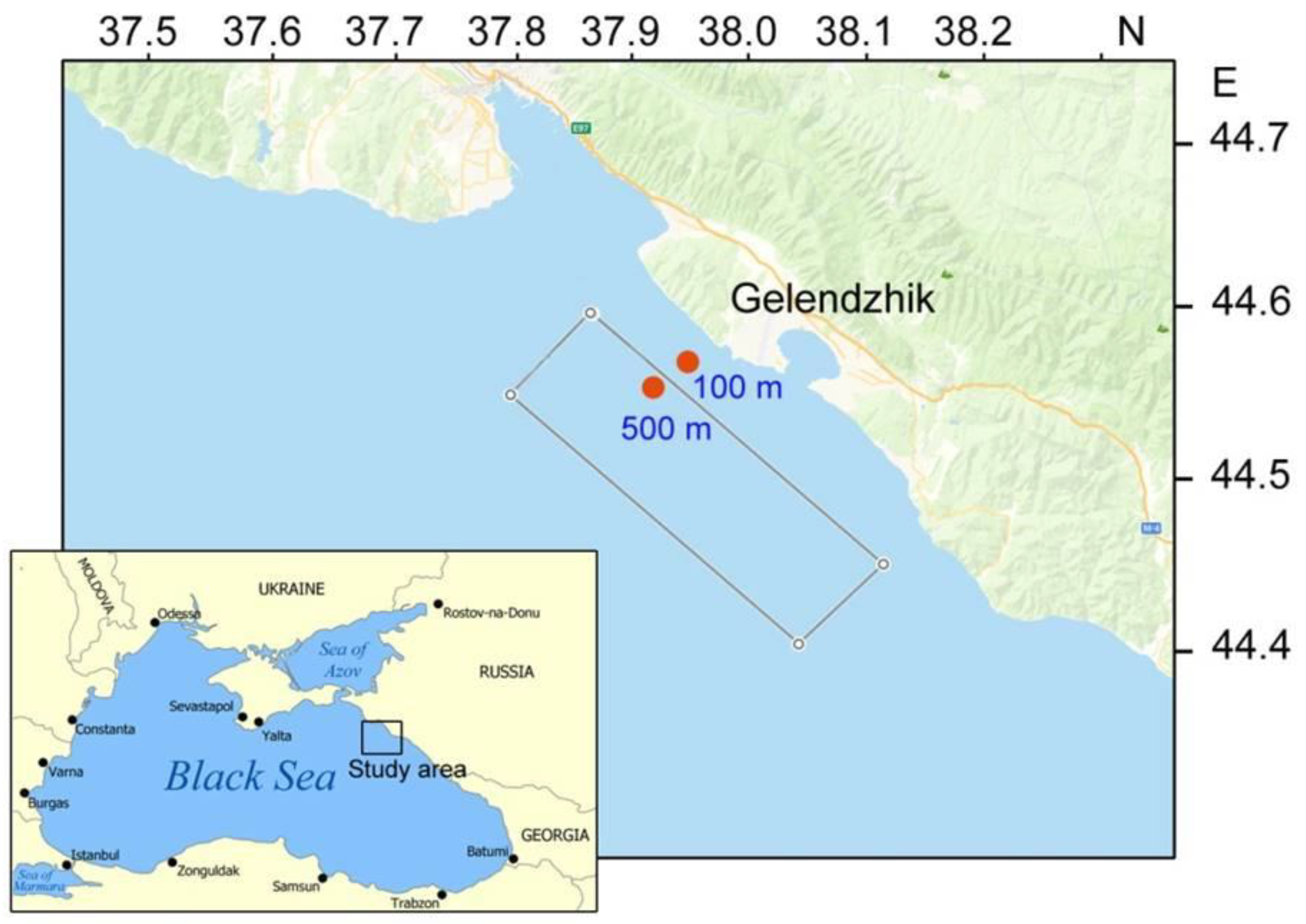
2.1. Field Sampling
2.2. Remote Sensing Data
2.3. Meteorological Data
3. Results
3.1. Wind on the Shelf and Adjacent Area
3.2. Hydrological Structure
3.3. Chl Dynamics in the Open Waters
3.4. Species Composition of Phytoplankton in the Shelf and Slope Areas
3.5. Cells Abundance
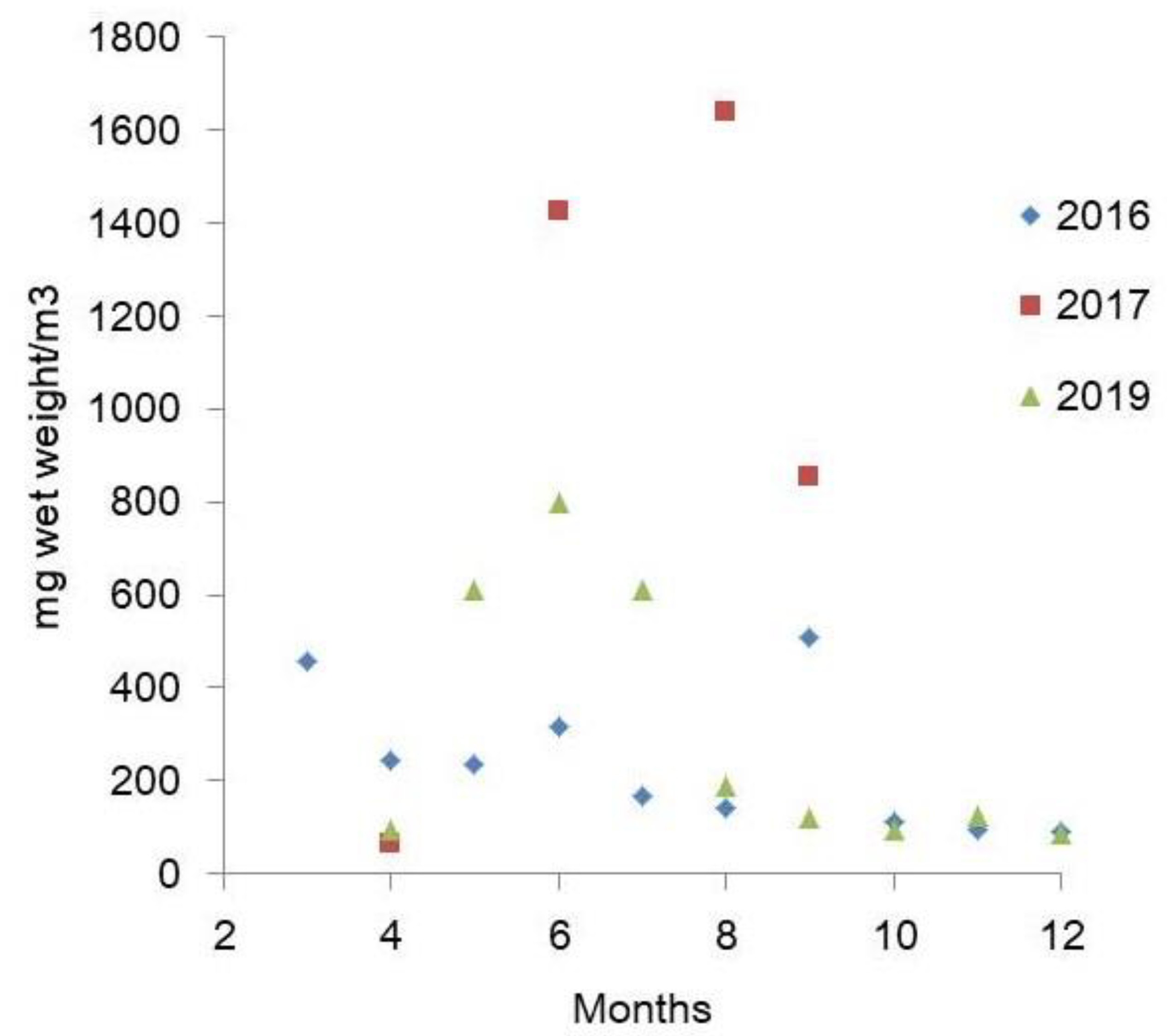
3.6. Biomass
3.7. Effect of Wind on Phytoplankton in the Slope Area
4. Discussion
4.1. Wind Effect on Annual Chl Dynamics
4.2. The Structure of Phytoplankton
4.3. Wind Regime
4.4. Annual Dynamics of Phytoplankton
4.5. Wind Effect on Annual Dynamics of Phytoplankton
5. Conclusions
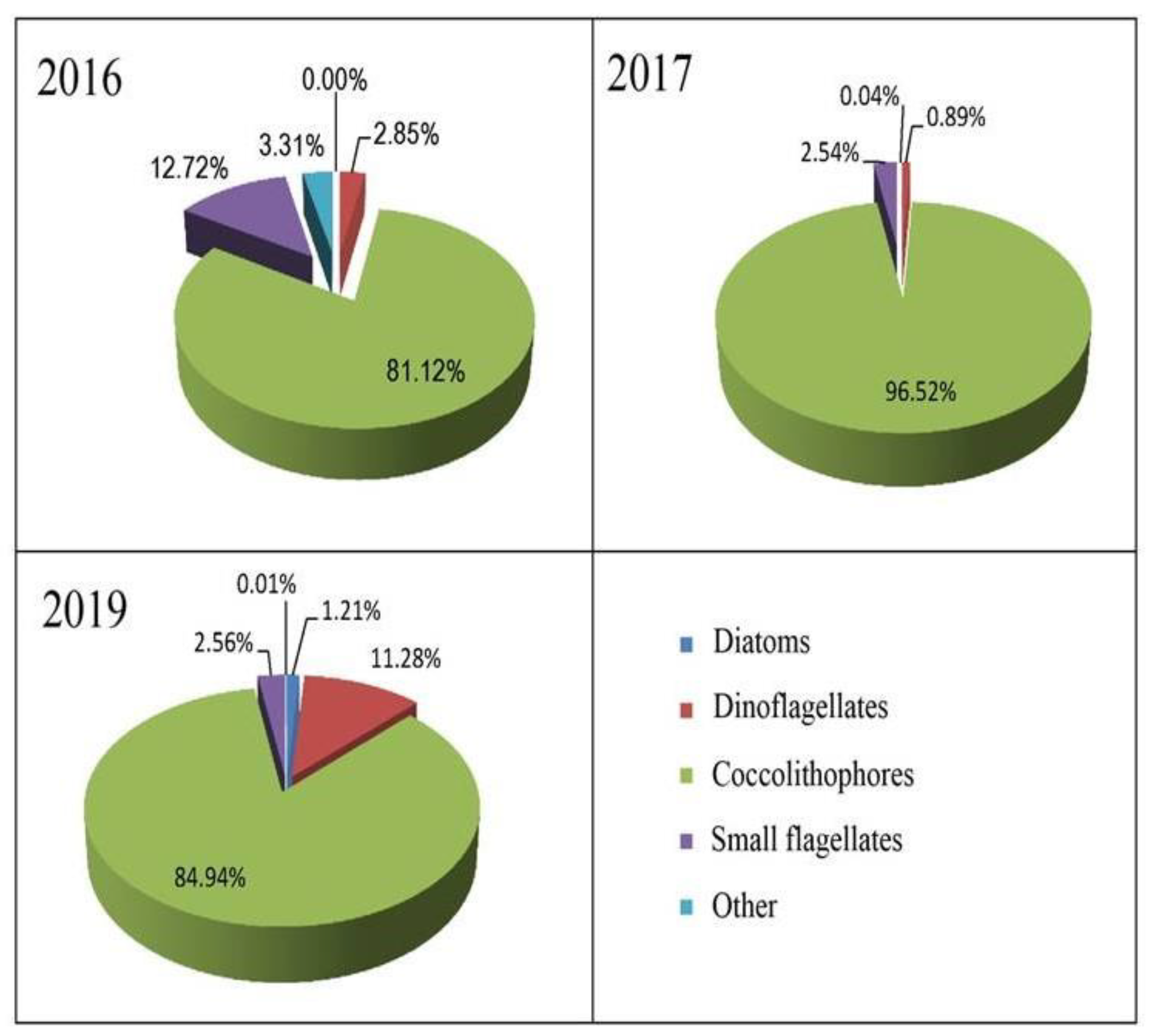
- The species composition of phytoplankton has not undergone significant changes compared to previous years. The phytoplankton numerical abundance was determined by coccolithophore Emiliania huxleyi, small flagellates, and diatoms. Diatoms, coccolithophores, and dinoflagellates formed the biomass.
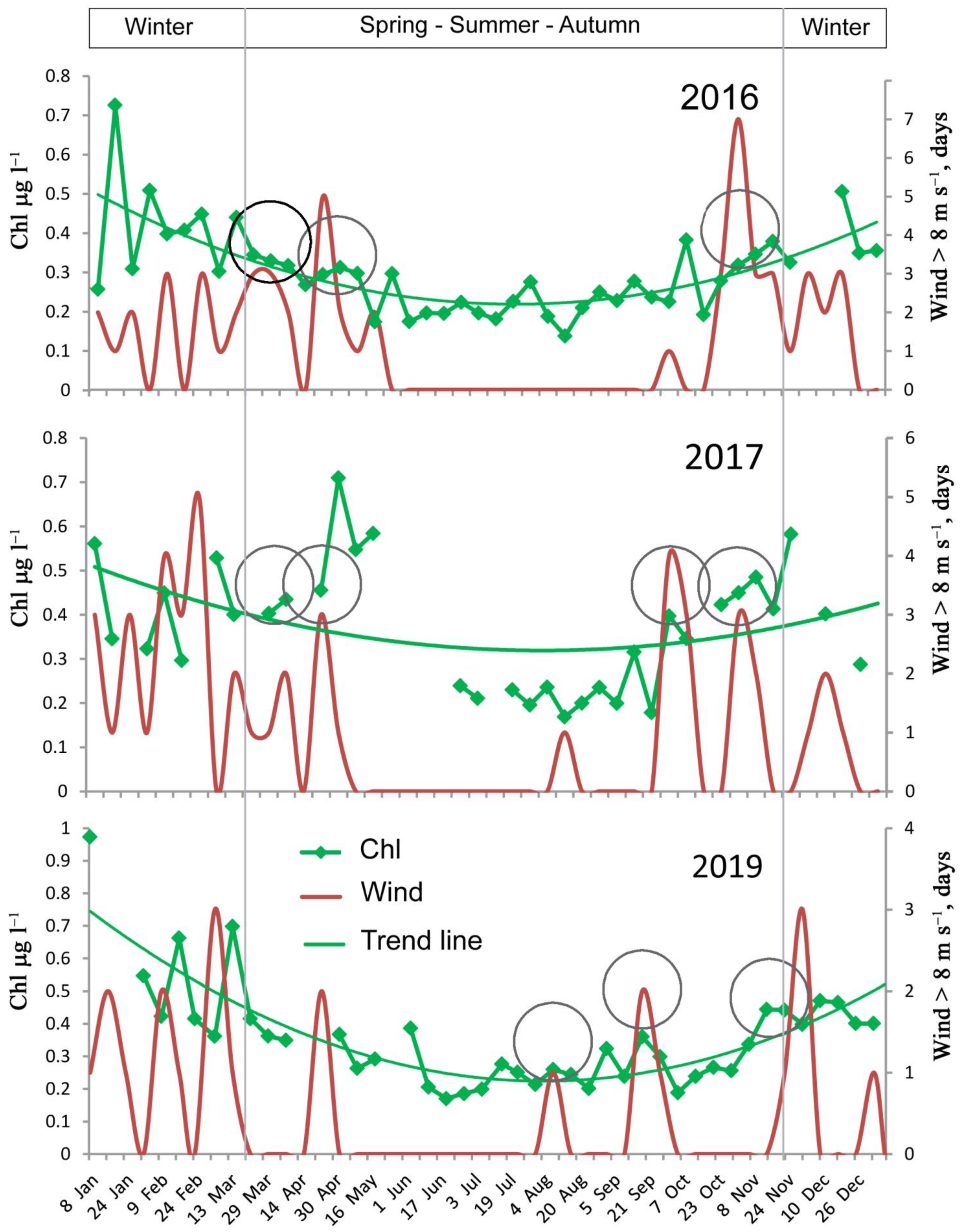
- The annual dynamics of satellite-derived Chl followed a U-shaped curve with a minimum in summer. Chl peaks are recorded in spring and autumn, and sometimes in summer. During the stratified water column period, strong winds regularly lead to a detectible increase in Chl. In the unstratified water period, a relationship between wind mixing and the amount of phytoplankton was not found.
- The annual dynamics of phytoplankton had the following pattern: small diatoms (spring) → coccolithophores (late spring, early summer) → large diatoms (summer, autumn). Such a pattern was typical for the previous decades.
- The combined effect of sustained offshore wind and strong current may cause bloom of diatoms during the stratified water period, even if the wind velocity is moderate.
Supplementary Materials
Author Contributions
Funding
Institutional Review Board Statement
Informed Consent Statement
Conflicts of Interest
References
- Volk, T.; Hoffert, M.I. Ocean carbon pumps: Analysis of relative strengths and efficiencies in ocean-driven atmospheric CO2 changes. In The Carbon Cycle and Atmospheric CO2 Natural Variations Archean to Present; Geophysical Monograph Series; Sundquist, E.T., Broecker, W.S., Eds.; American Geophysical Union: Washington, DC, USA, 1985; Volume 32, pp. 99–110. [Google Scholar]
- Sarmiento, J.L.; Gruber, N. Ocean Biogeochemical Dynamics; Princeton University Press: Princeton, NJ, USA, 2006; p. 526. [Google Scholar]
- Le Quéré, C.; Andrew, R.M.; Friedlingstein, P.; Sitch, S.; Hauck, J.; Pongratz, J.; Pickers, P.A.; Korsbakken, J.I.; Peters, G.P.; Canadell, J.G.; et al. Global Carbon Budget 2018. Earth Syst. Sci. Data 2018, 10, 2141–2194. [Google Scholar] [CrossRef] [Green Version]
- Field, C.B.; Behrenfeld, M.J.; Randerson, J.T.; Falkowski, P. Primary production of the biosphere: Integrating terrestrial and oceanic components. Science 1998, 281, 237–240. [Google Scholar] [CrossRef] [PubMed] [Green Version]
- Falkowski, P.; Scholes, R.J.; Boyle, E.; Canadell, J.; Canfield, D.; Elser, J.; Gruber, N.; Hibbard, K.; Högberg, P.; Linder, S.; et al. The Global Carbon Cycle: A Test of Our Knowledge of Earth as a System. Science 2000, 290, 291–296. [Google Scholar] [CrossRef] [PubMed] [Green Version]
- Smetacek, V. Diatoms and the ocean carbon cycle. Protist 1999, 150, 25–32. [Google Scholar] [CrossRef]
- Buesseler, K.O.; Michael, P.; Livingston, H.D.; Cochrant, K. Carbon and nitrogen export during the JGOFS North Atlantic Bloom Experiment estimated from 234Th:238U disequilibria. Deep Sea Res. 1992, 39, 1115–1137. [Google Scholar] [CrossRef]
- Milliman, J.D. Production and accumulation of calcium carbonate in the ocean: Budget of a non-steady state. Glob. Biogeochem. Cycles 1993, 7, 927–957. [Google Scholar] [CrossRef]
- Ryther, J.N.; Dunstan, W.M. Nitrogen, phosphorus, and eutrophication in the coastal marine environment. Science 1971, 171, 1008–1013. [Google Scholar] [CrossRef] [Green Version]
- Hecky, R.E.; Kilham, P. Nutrient limitation of phytoplankton in freshwater and marine environments: A review of recent evidence on the effects of enrichment. Limnol. Oceanogr. 1988, 33, 796–822. [Google Scholar] [CrossRef] [Green Version]
- Barton, A.D.; Lozier, M.S.; Williams, R.G. Physical controls of variability in North Atlantic phytoplankton communities. Limnol. Oceanogr. 2014, 60, 181–197. [Google Scholar] [CrossRef] [Green Version]
- Silkin, V.A.; Fedorov, A.V.; Flynn, K.J.; Paramonov, L.E.; Pautova, L.A. Protoplasmic streaming of chloroplasts enables rapid photoacclimation in large diatoms. J. Plankton Res. 2021, 43, 831–845. [Google Scholar] [CrossRef]
- Kiørboe, T. A Mechanistic Approach to Plankton Ecology; Princeton University Press: Princeton, NJ, USA, 2008; p. 224. [Google Scholar]
- Kiørboe, T. How zooplankton feed: Mechanisms, traits and trade-offs. Biol. Rev. Cam. Phil. Soc. 2011, 86, 311–339. [Google Scholar] [CrossRef]
- Ward, B.A.; Dutkiewicz, S.; Jahn, O.; Follows, M.J. A size-structured food-web model for the global ocean. Limnol. Oceanogr. 2012, 57, 1877–1891. [Google Scholar] [CrossRef]
- Flynn, K.J.; Kimmance, S.A.; Clark, D.R.; Mitra, A.; Polimene, L.; Wilson, W.H. Modelling the effects of traits and abiotic factors on viral lysis in phytoplankton. Front. Mar. Sci. 2021, 8, 667184. [Google Scholar] [CrossRef]
- Behrenfeld, M.J.; Halsey, K.H.; Boss, E.; Karp-Boss, L.; Milligan, A.J.; Peers, G. Thoughts on the evolution and ecological niche of diatoms. Ecol. Monogr. 2021, 91, e01457. [Google Scholar] [CrossRef]
- Behrenfeld, M.J.; Boss, E.; Halsey, K.H. Phytoplankton community structuring and succession in a competition-neutral resource landscape. ISME Commun. 2021, 1, 12. [Google Scholar] [CrossRef]
- Falkowski, P.G.; Oliver, M.J. Mix and match: How climate selects phytoplankton. Nat. Rev. Microbiol. 2007, 5, 813–819. [Google Scholar] [CrossRef] [PubMed]
- Young, R.; Zieger, S.; Babani, A.V. Global Trends in Wind Speed and Wave Height. Sci. Vol. 2011, 332, 451–455. [Google Scholar] [CrossRef]
- Mikaelyan, A.S.; Zatsepin, A.G.; Kubryakov, A.A. Effect of Mesoscale Eddy Dynamics on Bioproductivity of the Marine Ecosystems (Review). Phys. Oceanogr. 2020, 27, 590–618. [Google Scholar] [CrossRef]
- Silkin, V.A.; Pautova, L.A.; Giordano, M.; Chasovnikov, V.K.; Vostokov, S.V.; Podymov, O.I.; Pakhomova, S.V.; Moskalenko, L.V. Drivers of phytoplankton blooms in the northeastern Black Sea. Mar. Poll. Bull. 2019, 138, 274–284. [Google Scholar] [CrossRef]
- Sorokin, Y.I. The Black Sea Ecology and Oceanography; Backhuys Publishers: Leiden, The Netherlands, 2002; p. 875. [Google Scholar]
- Bodeanu, N.; Andrei, C.; Boicenco, L.; Popa, L.; Sburlea, A. A new trend of the phytoplankton structure and dynamics in the Romanian marine waters. Cercet. Mar. 2004, 35, 77–86. [Google Scholar]
- Moncheva, S.; Petrova-Karadjova, V.; Palasov, A. Harmful algal blooms along the Bulgarian Black Sea coast and possible patterns of fish and zoobenthic mortalities. In Harmful Marine Algal Blooms; Lavoisier Publ. Incorp: Paris, France, 1995; pp. 193–198. [Google Scholar]
- Moncheva, S.; Gotsis-Skretas, O.; Pagou, K.; Krastev, A. Phytoplankton Blooms in Black Sea and Mediterranean Coastal Ecosystems Subjected to Anthropogenic Eutrophication: Similarities and Differences. Estuar. Coast. Shelf 2001, 53, 281–295. [Google Scholar] [CrossRef] [Green Version]
- Velikova, V.; Moncheva, S.; Petrova, D. Phytoplankton dynamics and Red Tides (1987–1997) in the Bulgarian Black Sea. Water Sci. Technol. 1999, 39, 27–36. [Google Scholar] [CrossRef]
- Mikaelyan, A.S. Winter bloom of diatom Nitzschia delicatula in the open waters of the Black Sea. Mar. Ecol. Prog. Ser. 1995, 129, 241–251. [Google Scholar] [CrossRef]
- Oğuz, T.; Deshpande, A.G.; Malanotte-Rizzoli, P. The role of mesoscale processes controlling biological variability in the Black Sea coastal waters: Inferences from SeaWIFS-derived surface chlorophyll field. Cont. Shelf Res. 2002, 22, 1477–1492. [Google Scholar] [CrossRef]
- Zatsepin, A.G.; Baranov, V.I.; Kondrashov, A.A.; Korzh, A.O.; Kremenetskiy, V.V.; Ostrovskii, A.G.; Soloviev, D.M. Submesoscale Eddies at the Caucasus Black Sea Shelf and the Mechanisms of Their Generation. Oceanology 2011, 51, 554–567. [Google Scholar] [CrossRef]
- Kubryakov, A.A.; Stanichny, S.V.; Zatsepin, A.G.; Kremenetskiy, V.V. Long-Term Variations of the Black Sea Dynamics and Their Impact on the Marine Ecosystem. J. Mar. Syst. 2016, 163, 80–94. [Google Scholar] [CrossRef]
- Krivosheya, V.G.; Moskalenko, L.V.; Melnikov, V.A.; Skirta, A.Y. Effects of the Wind and Thermal Conditions Variability on the Structure and Dynamics of the Seawater in the Northeastern Black Sea. Oceanology 2012, 52, 453–466. [Google Scholar] [CrossRef]
- Belogorskaya, E.V.; Kondratieva, T.M. The Distribution of the Phytoplankton in the Black Sea. Studies of the Plankton of the Black Sea and the Asov Sea; Naukova Dumka: Kiev, Ukraine, 1965; pp. 36–58. (In Russian) [Google Scholar]
- Georgieva, L.V. Phytoplankton. Species composition and dynamics. In Plankton of the Black Sea; Kovalev, A.V., Finenko, Z.Z., Eds.; Naukova Dymka: Kiev, Ukraine, 1993; pp. 31–55. (In Russian) [Google Scholar]
- Mashtakova, G.P.; Roukhiyainen, M.I. Seasonal dynamics of phytoplankton. In Basis of Productivity in the Black Sea; Greeze, V.N., Ed.; Naukova Dumka: Kiev, Ukraine, 1979; pp. 85–87. (In Russian) [Google Scholar]
- Zernova, V.V.; Nezlin, N.P. Seasonal changes in phytoplankton in the north-eastern part of the Black Sea during 1978. In Seasonal Changes in Plankton of the Black Sea; Vinogradov, M.E., Ed.; Nauka: Moscow, Russia, 1983; pp. 12–25. (In Russian) [Google Scholar]
- Vershinin, A.; Moruchkov, A.; Sukhanova, I.; Kamnev, A.N.; Pankov, S.; Morton, S.; Ramsdell, J. Seasonal changes in coastal phytoplankton at Bolšoj Utriš (northeast Black Sea) in 2001–2002. Oceanology 2004, 44, 399–405. [Google Scholar]
- Mikaelyan, A.S.; Pautova, L.A.; Pogosyan, S.I.; Suchanova, I.N. Summer bloom of coccolithophorids in the northeastern Black Sea. Oceanology 2005, 45, 127–138. [Google Scholar]
- Pautova, L.A.; Mikaelyan, A.S.; Silkin, V.A. The structure of plankton community in shelf waters of north-eastern part of the Black Sea in the period of mass bloom of Emiliania huxleyi in 2002–2005. Oceanology 2007, 47, 408–417. [Google Scholar] [CrossRef]
- Silkin, V.A.; Pautova, L.A.; Pakhomova, S.V.; Lifanchuk, A.V.; Yakushev, E.V.; Chasovnikov, V.K. Environmental control on phytoplankton community structure in the NE Black Sea. J. Exp. Mar. Biol. Ecol. 2014, 461, 267–274. [Google Scholar] [CrossRef]
- Mikaelyan, A.S.; Pautova, L.A.; Chasovnikov, V.K.; Mosharov, S.A.; Silkin, V.A. Alternation of diatoms and coccolithophores in the northeastern Black Sea: A response to nutrient changes. Hydrobiologia 2015, 755, 89–105. [Google Scholar] [CrossRef]
- Sukhanova, I.N. The phenomenon of mass bloom of coccolitophorids in late autumn period in the Black Sea. RAS Rep. 1995, 340, 256–259. (In Russian) [Google Scholar]
- Kubryakov, A.A.; Zatsepin, A.G.; Stanichny, S.V. Anomalous summer-autumn phytoplankton bloom in 2015 in the Black Sea caused by several strong wind events. J. Mar. Syst. 2019, 194, 11–24. [Google Scholar] [CrossRef]
- Kubryakova, E.A.; Kubryakov, A.A.; Mikaelyan, A.S. Winter coccolithophore blooms in the Black Sea: Interannual variability and driving factors. J. Mar. Syst. 2021, 213, 103461. [Google Scholar] [CrossRef]
- Yunev, O.A.; Vedernikov, V.I.; Basturk, O.; Yilmaz, A.; Kideys, A.E.; Moncheva, S.; Konovalov, S.K. Long-term variations of surface chlorophyll a and primary production in the open Black Sea. Mar. Ecol. Prog. Ser. 2002, 230, 11–28. [Google Scholar] [CrossRef]
- Mikaelyan, A.S.; Chasovnikov, V.K.; Kubryakov, A.A.; Stanichny, S.V. Phenology and drivers of the winter-spring phytoplankton bloom in the open Black Sea: The application of Sverdrup’s hypothesis and its refinements. Prog. Oceanogr. 2017, 151, 163–176. [Google Scholar] [CrossRef]
- Kubryakov, A.A.; Bagaev, A.V.; Stanichny, S.V.; Belokopytov, V.N. Thermohaline structure, transport and evolution of the Black Sea eddies from hydrological and satellite data. Prog. Oceanogr. 2018, 167, 44–63. [Google Scholar] [CrossRef]
- Kubryakov, A.A.; Mikaelyan, A.S.; Stanichny, S.V. Extremely strong coccolithophore blooms in the Black Sea: The decisive role of winter vertical entrainment of deep water. Deep. Sea Res. Part I Oceanogr. Res. Pap. 2021, 125, 103554. [Google Scholar] [CrossRef]
- Kopelevich, O.; Burenkov, V.; Sheberstov, S.; Vazyulya, S.; Kravchishina, M.; Pautova, L.; Silkin, V.; Artemiev, V.; Grigoriev, A. Satellite monitoring of coccolithophore blooms in the Black Sea from ocean color data. Remote Sens. Environ. 2014, 146, 113–123. [Google Scholar] [CrossRef]
- Kiselev, I.A. Plankton of Seas and Continental Basins; Nauka: St. Petersburg, Russia, 1969; p. 657. (In Russian) [Google Scholar]
- Moncheva, S.; Parr, B. Manual for Phytoplankton Sampling and Analysis in the Black Sea. 2010. Available online: http://www.blacksea-commission.org (accessed on 15 October 2021).
- Tomas, C.R. (Ed.) Identifying Marine Phytoplankton; Academic Press: San Diego, CA, USA, 1997; p. 858. [Google Scholar]
- Throndsen, J.; Hasle, G.R.; Tangen, K. Norsk Kystplanktonflora; Almater Forlag AS: Oslo, Norway, 2003; p. 341. [Google Scholar]
- Hillebrand, H.; Durselen, C.; Kirschtel, D.; Pollingher, U.; Zohary, T. Biovolume calculation for pelagic and benthic microalgae. J. Phycol. 1999, 35, 403–424. [Google Scholar] [CrossRef]
- Tyrrell, T.; Merico, M. Emiliania huxleyi: Bloom observations and the conditions that induce them. In Coccolithophores from Molecular Processes to Global Impact; Thierstein, H.R., Young, J.R., Eds.; Springer: Berlin/Heidelberg, Germany, 2004; pp. 75–97. [Google Scholar]
- Kopelevich, O.V.; Burenkov, V.I.; Sheberstov, S.V.; Vazyulya, S.V.; Zavialov, S.P. Bio-optical characteristics of the Russian Seas from satellite ocean color data of 1998–2010. In Proceedings of the YI International Conference “Current Problems in Optics of Natural Waters (ONW 20011)”, St. Petersburg, Russia, 6–9 September 2011; pp. 181–182. [Google Scholar]
- Stanichnaya, R.G.; Stanichny, S.V.; Arashkevich, E.G. Regionally adapted algorithm for the recovery of chlorophyll aconcentration for the Black Sea, analysis of the reasonsfor the difference between satellite and contact data. Curr. Probl. Remote Sens. Earth Space 2020, 17, 29–37. [Google Scholar]
- Carlson, D.F.; Muscarella, P.A.; Gildor, H.; Lipphardt, B.L., Jr.; Fredj, E. How useful are progressive vector diagrams for studying coastal ocean transport? Limnol. Oceanogr. 2010, 8, 98–106. [Google Scholar] [CrossRef] [Green Version]
- Zatsepin, A.G.; Kremenetskiy, V.V.; Piotoukh, V.B.; Poyarkov, S.G.; Ratner, Y.B.; Soloviev, D.M.; Stanichnaya, R.G.; Stanichny, S.V.; Yakubenko, V.G. Formation of nearshore current in the Black Sea due to spatial non-uniformity of wind impact on the upper mixed layer. Oceanology 2008, 48, 1–17. [Google Scholar]
- Ivanov, V.A.; Belokopytov, V.N. Oceanography of the Black Sea; NAS of Ukraine Marine Hydrophysical Institute: Sevastopol, Crimea, 2011; p. 209. (In Russian)
- Finenko, Z.; Suslin, V.; Kovaleva, I. Seasonal and long-term dynamics of the chlorophyll concentration in the Black Sea according to satellite observations. Oceanology 2014, 54, 596–605. [Google Scholar] [CrossRef]
- Dennman, K.L.; Gargett, A.E. Time and space scales of vertical mixing and advection of phytoplankton in the upper ocean. Limnol. Oceanogr. 1983, 28, 801–815. [Google Scholar] [CrossRef]
- Pan, G.; Chai, F.; Tang, D.; Wang, D. Marine phytoplankton biomass responses to typhoon events in the South China Sea based on physical-biogeochemical model. Ecol. Model. 2017, 356, 38–47. [Google Scholar] [CrossRef]
- Liu, Y.; Tang, D.; Evgeny, M. Chlorophyll Concentration Response to the Typhoon Wind-Pump Induced Upper Ocean Processes Considering Air–Sea Heat Exchange. Remote Sens. 2019, 11, 1825. [Google Scholar] [CrossRef] [Green Version]
- Sverdrup, H.U. On conditions for the vernal blooming of phytoplankton. J. Cons. Int. Explor. Mer. 1953, 18, 287–295. [Google Scholar] [CrossRef]
- Chiswell, S.M. Annual cycles and spring blooms in phytoplankton: Don’t abandon Sverdrup completely. Mar. Ecol. Prog. Ser. 2011, 443, 39–50. [Google Scholar] [CrossRef] [Green Version]
- Lindemann, C.; John, M.A.S. A seasonal diary of phytoplankton in the North Atlantic. Front. Mar. Sci. 2014, 1, A37. [Google Scholar] [CrossRef] [Green Version]
- Gohin, F.; Bryère, P.; Griffiths, J.W. The exceptional surface turbidity of the North-West European shelf seas during the stormy 2013–2014 winter: Consequences for the initiation of the phytoplankton blooms? J. Mar. Syst. 2015, 148, 70–85. [Google Scholar] [CrossRef] [Green Version]
- Ueyama, R.; Monger, B.C. Wind-induced modulation of seasonal phytoplankton blooms in the North Atlantic derived from satellite observations. Limnol. Oceanogr. 2005, 50, 1820–1829. [Google Scholar] [CrossRef]
- Titov, V.B. The Effect of the Long-Term Variations in Climate Conditions on the Hydrological Structure and Ecology of the Black Sea. Water Resour. 2004, 31, 369–375. [Google Scholar] [CrossRef]
- Sukhanova, I.N.; Mikaelyan, A.S.; Georgieva, L.V. Spatial distribution and temporal variations of phytoplankton in the Black Sea (March–April 1988) during the spring bloom period. In Studies of Phytoplankton Using Monitoring System in the Baltic Sea and Other Seas of the USSR; Tsyban, A.V., Ed.; Gidromet: Moscow, Russia, 1991; pp. 135–152. (In Russian) [Google Scholar]
- Eker-Develi, E.; Kideys, A.E. Distribution of phytoplankton in the southern Black Sea in summer 1996, spring and autumn 1998. J. Mar. Syst. 2003, 39, 203–211. [Google Scholar] [CrossRef]
- Sommer, U.; Gliwicz, Z.M.; Lampert, W.; Duncan, A. The PEG-model of seasonal succession of planktonic events in fresh waters. Arch. Hydrobiol. 1986, 106, 433–471. [Google Scholar]
- Siegel, D.A.; Doney, S.C.; Yoder, J.A. The North Atlantic spring phytoplankton bloom and Sverdrup’s critical depth hypothesis. Science 2002, 296, 730–733. [Google Scholar] [CrossRef] [PubMed]
- Sommer, U.; Adrian, R.; De Senerpont, D.L.; Elser, J.J.; Gaedke, U.; Ibelings, B.; Jeppesen, E.; Lürling, M.; Molinero, C.J.; Mooij, W.M.; et al. The Plankton Ecology Group (PEG) Model: Mechanisms driving plankton succession. Annu. Rev. Ecol. Evol. Syst. 2012, 43, 429–448. [Google Scholar] [CrossRef]
- Behrenfeld, M.J. Abandoning Sverdrup’s critical depth hypothesis on phytoplankton blooms. Ecology 2010, 91, 977–989. [Google Scholar] [CrossRef]
- Taylor, J.R.; Ferrari, R. Shutdown of turbulent convection as a new criterion for the onset of spring phytoplankton blooms. Limnol. Oceanogr. 2011, 56, 2293–2307. [Google Scholar] [CrossRef] [Green Version]
- Behrenfeld, M.J.; Boss, E.S. Resurrecting the Ecological Underpinnings of Ocean Plankton Blooms. Annu. Rev. Marine. Sci. 2014, 6, 167–194. [Google Scholar] [CrossRef] [Green Version]
- Arkhipkin, V.S.; Gippius, F.N.; Koltermann, K.P.; Surkova, G.V. Wind waves in the Black Sea: Results of a hind cast study. Nat. Hazards Earth Syst. Sci. 2014, 14, 2883–2897. [Google Scholar] [CrossRef] [Green Version]
- Wirtz, K.W. Who is eating whom? Morphology and feeding type determine the size relation between planktonic predators and their ideal prey. Mar. Ecol. Prog. Ser. 2012, 445, 1–12. [Google Scholar] [CrossRef] [Green Version]
- Stolte, W.; Riegman, R. A model approach for size-selective competition of marine phytoplankton for fluctuating nitrate and ammonium. J. Phycol. 1996, 32, 732–740. [Google Scholar] [CrossRef]
- Klausmeier, C.A.; Litchman, E.; Daufresne, T.; Levin, S.A. Optimal nitrogen-to-phosphorus stoichiometry of phytoplankton. Nature 2004, 429, 171–174. [Google Scholar] [CrossRef] [PubMed]
- Litchman, E.; Klausmeier, C.A.; Yoshiyama, K. Contrasting size evolution in marine and freshwater diatoms. Proc. Nat. Acad. Sci. USA 2009, 106, 2665–2670. [Google Scholar] [CrossRef] [Green Version]
- Abakumov, A.I.; Silkin, V.A.; Pautova, L.A. Biomass dynamics of the phytoplankton under impact of the nutrient. Procedia Environ. Sci. 2011, 8, 105–110. [Google Scholar] [CrossRef] [Green Version]
- Mikaelyan, A.S.; Kubryakov, A.A.; Silkin, V.A.; Pautova, L.A.; Chasovnikov, V.K. Regional climate and patterns of phytoplankton annual succession in the open waters of the Black Sea. Deep-Sea Res. Part I 2018, 142, 44–57. [Google Scholar] [CrossRef]
- Morel, A.; Bricaud, A. Theoretical results concerning light absorption in a discrete medium, and application to specific absorption of phytoplankton. Deep Sea Res. 1981, 28, 1375–1393. [Google Scholar] [CrossRef]
- Finkel, Z.V.; Irwin, A.J. Modeling size-dependent photo synthesis: Light absorption and the allometric rule. J. Theor. Biol. 2000, 204, 361–369. [Google Scholar] [CrossRef] [PubMed] [Green Version]
- Finkel, Z.V. Light absorption and size scaling of light-limited metabolism in marine diatoms. Limnol. Oceanogr. 2001, 46, 86–94. [Google Scholar] [CrossRef] [Green Version]
- Finkel, Z.V.; Irwin, A.J.; Schofield, O. Resource limitation alters the ¾ size scaling of metabolic rates in phytoplankton. Mar. Ecol. Prog. Ser. 2004, 273, 269–279. [Google Scholar] [CrossRef]
- Yunev, O.A.; Carstensen, J.; Stelmakh, L.V.; Belokopytov, V.N.; Suslin, V.V. Reconsideration of the phytoplankton seasonality in the open Black Sea. Limnol. Oceanogr. Lett. 2021, 6, 51–59. [Google Scholar] [CrossRef]
- Duysens, L.N.M. The flattening of the absorption spectra of suspensions as compared to that of solutions. Biochim. Biophys. Acta 1956, 19, 1–12. [Google Scholar] [CrossRef]
- Key, T.; McCarthy, A.; Campbell, D.A.; Six, C.; Roy, S.; Finkel, Z.V. Cell size trade-offs govern light exploitation strategies in marine phytoplankton. Env. Microbiol. 2010, 12, 95–104. [Google Scholar] [CrossRef] [PubMed]
- Agusti, S. Allometric scaling of light absorption and scattering by phytoplankton cells. Can. J. Fish. Aquat. Sci. 1991, 48, 763–767. [Google Scholar] [CrossRef]


| Taxon | 2016 | 2017 | 2019 | |||
|---|---|---|---|---|---|---|
| N | % | N | % | N | % | |
| Bacillariophyceae | 14 | 18.9 | 27 | 23.7 | 25 | 27.5 |
| Dinophyceae | 51 | 68.9 | 74 | 64.9 | 55 | 60.4 |
| Prymnesiophyceae | 4 | 5.4 | 6 | 5.2 | 5 | 5.5 |
| Cryptophyceae | 1 | 1.4 | 1 | 0.9 | 1 | 1.1 |
| Dictyochophyceae | 3 | 4.0 | 4 | 3.5 | 3 | 3.3 |
| Chlorophyceae | - | - | 1 | 0.9 | 1 | 1.1 |
| Euglenophyceae | 1 | 1.4 | 1 | 0.9 | 1 | 1.1 |
| Total | 74 | 100 | 114 | 100 | 91 | 100 |
| Species | 2016 | 2017 | 2019 |
|---|---|---|---|
| Dominants | |||
| Small flagellates (size 6–10 µm) | 2.1 × 10⁶ June | 8.4 × 10⁵ June | 1.0 × 10⁶ June, August, September |
| Emiliania huxleyi | 1.1–1.2 × 10⁶ April–May | 7.7 × 10⁶ June | 3.3–3.7 × 10⁶ May–June |
| Pseudosolenia calcar-avis | 2.1 × 10⁴ June | 1.1 × 10⁵ August | 9.6 × 10³ July |
| Pseudo-nitzschia delicatissima | - | - | 1.1 × 10⁶ May |
| Proboscia alata | - | - | 1.8 × 10³ September |
| Sub-dominants | |||
| Thalassionema nitzschioides | 6.4–6.1 × 10³ June, September | 1.2 × 10⁴ August | 3.4 × 10³ May |
| Cryptomonas sp. | - | 2.3 × 10⁴ September | 3.6 × 10⁴ June |
| Gyrodinium fusiforme | 1.1 × 10⁴ June | 1.0 × 10³ August | 2.3 × 10⁴ May |
| Scrippsiella acuminata | 7.8 × 10³ June | 2.2 × 10³ August | 8.2 × 10³ June |
| Prorocentrum micans | 1.4 × 10³ November | 1.2 × 10³ July | 1.4 × 10³ November |
| Prorocentrum cordatum | 2.4 × 10² June, July, September | - | 1.0 × 10³ November |
| Prorocentrum balticum | - | - | 4.4 × 10³ May |
| Pseudo-nitzschia delicatissima | 1.8 × 10⁴ August | 3.6 × 10⁴ August | - |
| Year | March | April | May | June | July | August | September | October | November | December |
|---|---|---|---|---|---|---|---|---|---|---|
| 2016 | 456.3 | 245.9 | 236.6 | 317.4 | 166.3 | 143.4 | 506.8 | 110.8 | 95.3 | 92.0 |
| 2017 | 60.6 | 1428.5 | 1638.5 | 854.1 | ||||||
| 2019 | 94.0 | 610.1 | 801.2 | 610.1 | 190.1 | 120.6 | 93.1 | 122.7 | 86.4 |
| Taxon | March | April | May | June | July | August | September | October | November | December |
|---|---|---|---|---|---|---|---|---|---|---|
| 2016 | ||||||||||
| Diatoms | 1.0 | 0 | 0 | 5.8 | 0.6 | 4.6 | 0.7 | 3.1 | 6.5 | 0.1 |
| Dinoflagellates | 81.5 | 6.7 | 2.8 | 42.6 | 9.7 | 41.1 | 15.2 | 61.2 | 24.8 | 29.6 |
| E. huxleyi | 9.0 | 89.7 | 81.1 | 36.6 | 72.9 | 10.9 | 0 | 7.9 | 44.1 | 50.8 |
| Dinobryon balticum | - | - | - | - | - | - | 80.0 | - | - | - |
| Small flagellates | 5.8 | 2.8 | 12.7 | 13.0 | 14.1 | 32.6 | 16.7 | 14.8 | 20.2 | 8.0 |
| 2017 | ||||||||||
| Diatoms | 0 | 0 | 98.5 | 97.2 | ||||||
| Dinoflagellates | 4.8 | 0.9 | 0.9 | 1.2 | ||||||
| E. huxleyi | 82.5 | 96.5 | 0.3 | 13.0 | ||||||
| Small flagellates | 11.8 | 2.5 | 0.5 | 1.3 | ||||||
| 2019 | ||||||||||
| Diatoms | 4.8 | 0.35 | 1.2 | 52.0 | 14.0 | 5.0 | 0.7 | 18.3 | ||
| Dinoflagellates | 20.3 | 9.2 | 11.3 | 23.0 | 37.3 | 17.3 | 7.0 | 54.3 | ||
| E. huxleyi | 36.8 | 87.8 | 84.9 | 17.7 | 24.4 | 29.0 | 74.5 | 4.6 | ||
| Small flagellates | 38.0 | 2.6 | 2.6 | 7.2 | 27.0 | 48.6 | 17.7 | 29.2 | ||
Publisher’s Note: MDPI stays neutral with regard to jurisdictional claims in published maps and institutional affiliations. |
© 2021 by the authors. Licensee MDPI, Basel, Switzerland. This article is an open access article distributed under the terms and conditions of the Creative Commons Attribution (CC BY) license (https://creativecommons.org/licenses/by/4.0/).
Share and Cite
Silkin, V.; Mikaelyan, A.S.; Pautova, L.; Fedorov, A. Annual Dynamics of Phytoplankton in the Black Sea in Relation to Wind Exposure. J. Mar. Sci. Eng. 2021, 9, 1435. https://doi.org/10.3390/jmse9121435
Silkin V, Mikaelyan AS, Pautova L, Fedorov A. Annual Dynamics of Phytoplankton in the Black Sea in Relation to Wind Exposure. Journal of Marine Science and Engineering. 2021; 9(12):1435. https://doi.org/10.3390/jmse9121435
Chicago/Turabian StyleSilkin, Vladimir, Alexander S. Mikaelyan, Larisa Pautova, and Alexey Fedorov. 2021. "Annual Dynamics of Phytoplankton in the Black Sea in Relation to Wind Exposure" Journal of Marine Science and Engineering 9, no. 12: 1435. https://doi.org/10.3390/jmse9121435