A Comprehensive Approach to Account for Weather Uncertainties in Ship Route Optimization

Abstract

This work aims at defining in a probabilistic manner objectives and constraints typically considered in route optimization systems. Information about weather-related uncertainties is introduced by adopting ensemble forecast results. Classical reliability methods commonly used in structural analysis are adopted, allowing to achieve a simple yet effective evaluation of the probability of failure and the variability associated with the predicted fuel consumption and time of arrival. A quantitative example of application is provided, taking into consideration one of the main North Atlantic routes.

1. Introduction

The selection of the most appropriate path for a ship to sail towards the destination has been a concern since the ancient times of maritime history. The degrading effect of environmental loads on vessel performance and their potential risk to its operability has been known since the early stages of navigation. Systematic collection of weather information has helped seafarers since the 18th century to reduce voyage time, but it is only in the second half of the 20th century that formal numerical techniques, initially based on the isochrone method [1], have been proposed to automatically identify the most favourable path.

Several approaches have been developed along the decades, with a sharp increase since the beginning of the new century as thoroughly depicted in [2,3]. The main concern has been on keeping the multi-objective nature of the optimization problem [4,5,6]. The objectives to be optimized typically encompass fuel consumption, voyage duration, and an index representing navigation safety. A common aspect of almost all of the proposed methods is to consider the prediction of environmental loads along the route as deterministic, even if the voyage may take several days. Nevertheless, the weather forecast is affected by uncertainties [7], which are nowadays to be mostly attributed to the inaccurate and partial knowledge about the initial conditions as third-generation numerical weather prediction models have achieved a high level of model accuracy. Only uncertainties related to the significant wave height and the wave period are accounted in this work for the sake of clarity, however, effortless extensions are possible, such as considering the effect of wind [8].

Ensemble forecasts [9,10,11] represent an effective technique to both improve the long term (more than 4–6 days) weather prediction and to assess its uncertainties, also providing their integral quantification in terms of standard deviations of the weather parameters. In its standard form, ensemble forecast consists of multiple runs of the numerical prediction models applying small perturbations to the initial conditions in order to evaluate their impact on the forecast. If not properly accounted for, the difference between the predicted and the actual weather conditions may counteract the effort made in the optimization of the route.

Pioneering work in this direction has been presented in [12], making use of ensemble forecasts to select the final route; however, ensemble forecasts were only used to evaluate the robustness of the selected route, ensuring that the constraints were not violated in a pre-defined number of cases. Applications to specific shipping sectors can be found in [13] for long term scheduling of LNG ships and in [14] which accounts for weather uncertainties for the development of speed optimization strategies in planning the operations of offshore supply vessels. In [15], uncertainties related to weather were considered on a two stage-optimization process: firstly, considering a classical multi-objective optimization of fuel and expected time of arrival (ETA), and secondly, selecting the route that minimizes the fuel consumption with a given probability of arriving on time. In [16], the effect of the uncertainty of weather forecasts in ship fuel consumption has been quantified along the ship routes.

A comprehensive and flexible way to incorporate uncertainties in the optimisation process is still missing, and the present work aims at filling this gap by proposing a method, potentially applicable to any voyage optimization algorithm, to evaluate uncertainties in the objectives and constraints typically accounted in ship routing. Section 2 presents the probabilistic approach considered, Section 3 describes the method to obtain the risk associated with a specific route, the required fuel consumption, and the expected voyage duration, each represented by a single value (similarly to the ones used in deterministic approaches) but accounting for weather uncertainties. An example of application on a north Atlantic crossing route is provided in Section 4, while conclusions and final remarks are discussed in Section 5.

2. Probabilistic Approach

The method assumes the knowledge of the mean values and the variances (or standard deviations) of the uncertain weather parameters along the route, e.g., significant wave height $H_S$, mean period $T_m$ (or peak period $T_P$), and mean relative wave direction ${\chi }_m$, as well as the availability of a tool to estimate the required seakeeping responses, the fuel consumption, and the ship speed in the given weather conditions and for the imposed engine settings (typically RPM). The uncertain variables are considered normally distributed. Other sources of uncertainties not due to weather conditions are, for instance, model uncertainties in the estimation of ship responses [17,18,19], but also related to the attitude of the shipmaster and the engine control strategy adopted [20,21,22].

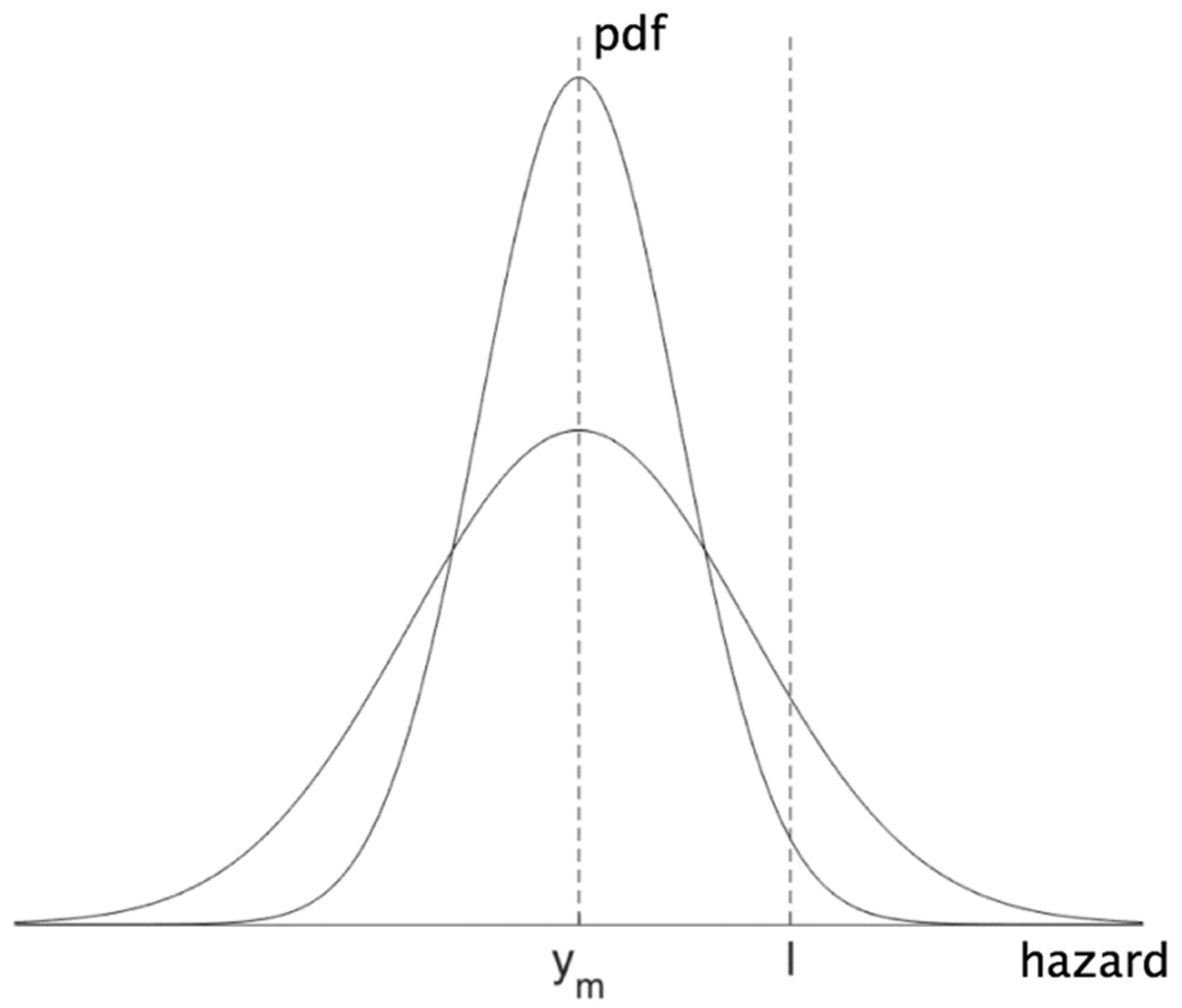
2.1. Navigational Risk

A probabilistic approach to navigational risk requires a robust methodology to estimate, at any given location along the route, the probability that any of the possible occurring risks will exceed a determined acceptable level $l$.

Consider a generic hazard (e.g., a seakeeping response) quantitatively definable by a value $y$. The value $y$ may represent, for instance, a significant vertical acceleration at the bridge, the root mean square of roll angle [23], or the probability of green water [24]. The response $y$ can be expressed as a function of a set of deterministic variables $\mathit{X}=\left(x_1,\dots ,x_i,\dots ,x_{n_d}\right)$ (e.g., ship main dimensions) and a set of uncertain variables $\tilde{\mathit{X}}=\left({\tilde{x}}_1,\dots ,{\tilde{x}}_i,\dots ,{\tilde{x}}_{n_u}\right)$ (e.g., weather parameters), and a black-box model for the estimation of $y$ is available:

$$y=y\left(\mathit{X},\tilde{\mathit{X}}\right)$$

(1)

By expanding in Taylor series around the mean values of the uncertain variables ${\tilde{\mathit{X}}}_m=\left({\tilde{x}}_m{}_1,\dots ,{\tilde{x}}_m{}_i,\dots ,{\tilde{x}}_{m_{n_u}}\right)$, the response can be approximated in the first order as:

$$y\left(\mathit{X},\tilde{\mathit{X}}\right)=y\left(\mathit{X},{\tilde{\mathit{X}}}_m\right)+{\displaystyle \sum }\frac{\partial y}{\partial {\tilde{x}}_i}\left({\tilde{x}}_i-{\tilde{x}}_{m_i}\right)$$

(2)

The ship operations are considered safe if the response $y$ does not exceed a limit value $l$. A limit state function can thus be defined as:

$$g=\frac{l-y}{l}$$

(3)

The navigation is to be considered unsafe if the limit state function is negative $g<0$. Assuming $l$ to be constant for a given response, from the Taylor approximation it is straightforward to obtain an estimation of the expected value and the variance for the limit state function:

$$\begin{array}{c}{\mu }_g=E\left[g\right]\approx g\left({\tilde{\mathit{X}}}_m,\mathit{X}\right)\\ {\sigma }_g^2=Var\left[g\right]={\displaystyle \sum }{\left(\frac{\partial g}{\partial {\tilde{x}}_i}\right)}^2{\sigma }_{{\tilde{x}}_i}^2+{\displaystyle {\displaystyle \sum }_{i\ne j}}\frac{\partial g}{\partial {\tilde{x}}_i}\frac{\partial g}{\partial {\tilde{x}}_j}{\rho }_{ij}{\sigma }_{{\tilde{x}}_i}{\sigma }_{{\tilde{x}}_j}\end{array}$$

(4)

where $\frac{\partial g}{\partial {\tilde{x}}_i}$ is the partial derivative of the limit state function with respect to the uncertain variables, and ${\sigma }_{{\tilde{x}}_i}$ is the standard deviation of the variables.

If only uncertainties in the significant wave height $H_S$ and a reference wave period (e.g., $T_P$) are considered, while all other variables are deterministic and included in $\widehat{\mathit{X}}$, the previous equations reduce to:

$$\begin{array}{c}{\mu }_g=E\left[g\right]\approx g\left(H_S{}_m,T_P{}_m,\widehat{\mathit{X}}\right)\\ {\sigma }_g^2=Var\left[g\right]={\left(\frac{\partial g}{\partial H_S}\right)}^2{\sigma }_{H_S}^2+{\left(\frac{\partial g}{\partial T_P}\right)}^2{\sigma }_{T_P}^2+2\frac{\partial g}{\partial H_S}\frac{\partial g}{\partial T_P}\rho {\sigma }_{H_S}{\sigma }_{T_P} \end{array}$$

(5)

where the correlation coefficient $\rho$ between $H_S$ and $T_P$ can be estimated, for instance, from the scatter diagram of the North Atlantic, resulting in $\rho =0.575$.

Assuming Gaussian distribution of the uncertainties in the input variables, as a consequence of the first-order approximation approach adopted, the limit state function can also be described by a Gaussian distribution. Thus, the probability of unsafe operations $p\left(g<0\right)$ can then be estimated as:

$$p\left(g\le 0\right)=\mathsf{\Phi }\left(-\frac{{\mu }_g}{{\sigma }_g}\right)$$

(6)

where $\mathsf{\Phi }\left(x\right)$ is the normal cumulative density function [25].

It is worth noting that, since the method lacks formulation invariance, another definition of the limit state function with respect to Equation (3) may lead to different results when analytical solutions are not available.

In this work, considerations on navigation safety are limited to seakeeping responses, such as vertical acceleration at the bridge, lateral acceleration at a critical cargo location, roll, green water, and slamming, as is typical [26]. However, the concepts can be easily extended to other types of risk unrelated or limitedly related with weather, e.g., risk of collision or grounding, as far as an estimation model is available. Moreover, methods developed in the field of structural reliability also allow us to consider the limit value $l$ as an uncertain variable, though this is not considered in the present work.

2.2. Navigation Performance

In order to evaluate the voyage performance, two parameters are relevant to ensure efficient operations of the ship are typically accounted for: duration and fuel consumption. The essential preliminary step to assess the voyage performance and the associated uncertainties is to evaluate the time and fuel required to sail an elementary portion of the route (navigation performance) and their variabilities related to the uncertain input variables.

A tool to obtain the ship speed $V_S$ and the fuel consumption per nautical mile $F{C}_{nmi}$, given a set of deterministic variables $\mathit{X}$ and a set of uncertain variables $\tilde{\mathit{X}}$, is here assumed to be available and considered as a black-box (e.g., [27]). Thus, for each track $k$ in which the route is divided, one can always obtain the time $d_k$ and the fuel $F{C}_k$ required to sail the track:

$$\begin{array}{c}{d}_k\left(\mathit{X},\tilde{\mathit{X}}\right)=l_k/V_S\left(\mathit{X},\tilde{\mathit{X}}\right)\\ F{C}_k\left(\mathit{X},\tilde{\mathit{X}}\right)=F{C}_{nmi}\left(\mathit{X},\tilde{\mathit{X}}\right)l_k\end{array}$$

(7)

where $l_k$ is the length of the track in nautical miles. As for the case of navigational risk described in Section 2.1 that have in general complex, nonlinear, and not readily available analytical form, duration and consumptions can be linearized in a neighbour of the estimated value of the uncertain input variables, as:

$$\begin{array}{c}{d}_k\left(\mathit{X},\tilde{\mathit{X}}\right)=d_k\left(\mathit{X},{\tilde{\mathit{X}}}_m\right)+{\displaystyle \sum }\frac{\partial d_k}{\partial {\tilde{x}}_i}\left({\tilde{x}}_i-{\tilde{x}}_m\right)\\ F{C}_k\left(\mathit{X},\tilde{\mathit{X}}\right)=F{C}_k\left(\mathit{X},{\tilde{\mathit{X}}}_m\right)+{\displaystyle \sum }\frac{\partial F{C}_k}{\partial {\tilde{x}}_i}\left({\tilde{x}}_i-{\tilde{x}}_m\right)\end{array}$$

(8)

Assuming that the uncertain variables are normally distributed, with known variances ${\sigma }_{{\tilde{x}}_i}^2$ and correlation coefficients ${\rho }_{ij}$, the linearization allows the adoption of simple equations to compute the estimates ${\mu }_k$ and the variances ${\sigma }_k^2$ of the parameters, as:

$$\begin{array}{c}{\mu }_{d_k}=E\left[d_k\right]\approx d_k\left({\tilde{\mathit{X}}}_m,\mathit{X}\right)\\ {\mu }_{F{C}_k}=E\left[F{C}_k\right]\approx F{C}_k\left({\tilde{\mathit{X}}}_m,\mathit{X}\right)\\ {\sigma }_{d_k}^2=Var\left[d_k\right]={\displaystyle \sum }{\left(\frac{\partial d_k}{\partial {\tilde{x}}_i}\right)}^2{\sigma }_{{\tilde{x}}_i}^2+{\displaystyle {\displaystyle \sum }_{i\ne j}}\frac{\partial d_k}{\partial {\tilde{x}}_i}\frac{\partial d_k}{\partial {\tilde{x}}_j}{\rho }_{ij}{\sigma }_{{\tilde{x}}_i}{\sigma }_{{\tilde{x}}_j}\\ {\sigma }_{F{C}_k}^2=Var\left[F{C}_k\right]={\displaystyle \sum }{\left(\frac{\partial F{C}_k}{\partial {\tilde{x}}_i}\right)}^2{\sigma }_{{\tilde{x}}_i}^2+{\displaystyle {\displaystyle \sum }_{i\ne j}}\frac{\partial F{C}_k}{\partial {\tilde{x}}_i}\frac{\partial F{C}_k}{\partial {\tilde{x}}_j}{\rho }_{ij}{\sigma }_{{\tilde{x}}_i}{\sigma }_{{\tilde{x}}_j}\end{array}$$

(9)

3. Definition of Optimization Objectives and Constraints

The previous section has discussed how to obtain a probabilistic estimation of the most significant quantities related to navigation performance and safety. A route optimisation software requires, however, integral quantities to define global objectives, enabling us to rank different route alternatives [28].

3.1. Safety Constraint

Risk constraints typically are defined in the form:

$$\{\begin{array}{c}if y\ge l \to c=false\\ else \to c=true \end{array}$$

(10)

where $y$ and $l$ are the value assumed by the generic hazard and is the maximum acceptable limit as previously defined, and $c$ is a Boolean that indicates whether the condition is acceptable (“true”) or not (“false”). This approach assumes a deterministic quantification of the hazard $y$. However, if uncertainties are affecting the quantification of the hazard, such an approach may be misleading. A hazard may assume the same mean value $y_m$, corresponding to the deterministic estimation but being affected by a different level of uncertainty.

In the graphical example in Figure 1, two probabilistic distributions of a hazard with the same mean value, but different standard deviation, are shown, as well as the limiting value $l$. Distributions are, in a first approximation, assumed as symmetric with respect to the mean value. For the narrower bell, corresponding to a lower level of uncertainty, the probability of $y\ge l$ is about $1.6\%$, while for the other case, the probability exceeds $10\%$. The latter may be unacceptable, but the deterministic approach is not able to identify such a dangerous situation. An extreme case happens when $y_m$ approaches $l$ and, consequently, the probability of $y\ge l$ approaches $50\%$.

The probabilistic approach offers much more flexibility in the definition of the constraints, which can be expressed in the form:

$$\{\begin{array}{c}if p\left(y\ge l\right)>p_R \to c=false\\ else \to c=true \end{array}$$

(11)

where $p_R$ is the risk-acceptable probability that the hazard will occur. For symmetric probabilistic distributions of the hazard, as in the previous example, $p_R=0.5$ the results are analogous to those of the deterministic approach. Typically, the acceptable risk differs depending, for instance, on the ship type. For instance, the acceptable risk $p_R$ of a passenger ship is lower than for a cargo ship, and this is lower than for a navy ship. The parameter $c$ can readily be used as a Boolean constraint to discard unsafe alternatives.

3.2. Risk Objective Function

The probability of the occurrence of an unsafe condition obtained in Equation (6) only refers to one of the possible $r$ hazards and to a specific location $k$ along the route, so it can be hereafter referred as $p_{k,r}$.

By assuming that the hazards are perfectly correlated, the probability of being caught in unsafe situations in a specific location can be estimated as the highest probability among the hazards considered. On the other hand, if the events are considered statistically independent, such probability could be obtained by the expression $1-\prod _{i=1}^{n_r}\left(1-p_{k,i}\right)$, where $n_r$ is the number of hazards. In the general case, it can be said that the probability of failure of the system falls between the range expressed in Equation (12). With a conservative approach, the upper bound can be taken [25]:

$${\max \left(p_{k,i}\right)|}_{i=1:n_r}\le p_k\le 1-{\displaystyle \prod }_{i=1}^{n_r}\left(1-p_{k,i}\right)$$

(12)

It is then clear that $p_k$ represents the probability of occurrence of any of the considered hazards in a given location along the route. Once $p_k$ is computed for all the control points along the route, these risk probabilities must be gathered in a single risk index as to be effectively used as an objective function to be minimized.

Depending on the requirements, different considerations may be done:

1. If the strategic objective is to prevent the ship to operate in conditions close to the maximum acceptable limit even for short periods, minimizing the highest $p_k$ is desired, thus a suitable risk index can be:

$$ris{k}_1=\max \left(p_j\right), j=1:n_k$$

(13)

where $n_k$ is the number of control points.

When comparing $ris{k}_1$ of two different routes, one alternative with smooth navigation for the greatest part of the voyage, but a short, particularly demanding event would have a higher risk index than a route where conditions are worse for most of the voyage.

This approach may be considered when the focus is on safety and the ultimate stresses of the system. However, if the constraints are appropriately set (e.g., a higher $p_R$ on Equation (11)), these can be sufficient to prevent dangerous conditions.

2. If, instead, comfort [29] is of primary importance, the average conditions along the route appear to be a more relevant indicator. In this case, a weighted average can be applied:

$$ris{k}_2=\frac{\sum d_k{p}_k}{d}$$

(14)

where $d_k$ refers to the time the ship takes to sail the track identified by the $k$ control point and $d$ is the duration of the voyage, being $d=\sum d_k$. When comparing $ris{k}_2$ of the two routes described at the previous point, the opposite would occur and the second route would have a higher risk index. The short passage through a storm is, in this case, hidden by the averaging, which may result in unexpected and undesired situations onboard

3. As to account for both the average conditions along the route and the most demanding ones, a generalized expression can be expressed in the following form:

$$ris{k}_3=w_{1}ris{k}_1+w_{2}ris{k}_2$$

(15)

where $w_1$ and $w_2$ are weights to be defined depending on the ship type and strategy. As a default setting, $w_1=w_2=0.5$ can be considered.

4. None of the previous methods appears adequate to reflect the level of severity felt onboard. A more appropriate solution could be obtained by assuming that the voyage results are less comfortable and more demanding if more challenging ship responses are faced for a relevant period, with respect to the duration of the route. Consequently, the navigation safety can be judged by analysing a restricted set of tracks that encompass a certain duration characterized by the higher probabilities of failure (higher values of $p_k$). The duration of the “relevant period” of time is arbitrarily set as equal to one-third of the voyage duration, though investigations have been carried out to adjust such a proportion by obtaining the feedback of experienced seafarers.

Similarly to case 2, a weighted average is performed, but in this case over the most severe cases, which account for $1/3$ of the voyage duration. Being $\widehat{k}$ the most severe control point for which $\sum d_{\widehat{k}}=d/3$:

$$ris{k}_4=\frac{\sum d_{\widehat{k}}{p}_{\widehat{k}}}{d/3}$$

(16)

3.3. Performance Objective Functions

Differently from the risk objective function that has been consistently defined as a probability of failure $R$, to express voyage performance, physical quantities must be maintained. Thus, a different approach is required. Using Equation (9), the estimates and variances of the fuel consumption and sailing time can be calculated for all the tracks. The corresponding integral values for the whole voyage $\mu$ and ${\sigma }^2$ can be obtained by summation of the previous, such as:

$$\begin{array}{c}\mu ={\displaystyle \sum _{k=1}^{n\_tracks}}{\mu }_k\\ {\sigma }^2={\displaystyle \sum _{i=1}^{n\_tracks}}{\sigma }_k^2+{\displaystyle \sum _{k=1}^{n\_tracks}}{\displaystyle \sum _{\begin{array}{c}j=1\\ j\ne k\end{array}}^{n\_tracks}}{\rho }_{kj}{\sigma }_k{\sigma }_j\end{array}$$

(17)

where ${\rho }_{kj}$ is, in this case, the correlation coefficient between the performance parameter (e.g., fuel consumption) on two different tracks.

Since all the other variables have been discussed in Section 2.2, the problem shifts to the assignment of realistic values to the correlation coefficient ${\rho }_{kj}$. The problem is not trivial; in fact, the interrelationship between, for instance, the fuel consumption on two different locations along the route depends on a large number of factors, such as the intensity of the atmospheric conditions affecting the area, the topography, and the manner in which the Shipmaster conducts the navigation. Intuitively, it can be reasonably postulated that the conditions of navigation are generally similar at a distance of a few miles, and therefore the performance is also similar. After several miles, the presence of land, passage through channels, and changes in weather conditions and engine settings can result in variations in the performance, and possible similarities have no systematic nature. Consequently, ${\rho }_{kj}$ is qualitatively higher for neighbour tracks and progressively reduces if the locations considered are far from one to the other.

Some preliminary analyses on routes in the North Atlantic suggested that the correlation can be neglected if the distance $d_{kj}$ between the considered locations is larger than $150 \mathrm{nmi}$. Thus, a simple form for the correlation coefficient linearly dependent on the distance is proposed as:

$${\rho }_{kj}=\{\begin{array}{c} 1-\frac{d_{kj}}{150} \mathrm{if} d_{kj}<150\\ 0 \mathrm{otherwise} \end{array}$$

(18)

By applying similar evaluations at different routes, it has been found that the correlation vanishes at a higher distance in milder weather conditions, due to the fact that weather-unrelated considerations prevail in those cases. The correlation coefficient did not appear significantly influenced by the ship type. The influence of other factors, such as weather severity and variability, must be studied in more detail to build a more generic and robust model for the correlation.

The proposed method allows an estimation of ${\mu }_d$, ${\mu }_{FC}$, ${\sigma }_d^2$ and ${\sigma }_{FC}^2$, where, within the Gaussian assumption of the distribution of the uncertain variables, the means correspond to the values obtained by a deterministic approach.

In practical terms, however, two values (mean and standard deviation) to define a single objective function are not convenient. It is then possible to make use of the additional information provided by the standard deviations to compute a predefined percentile, namely the values of the voyage duration and consumption, which have a given probability to be exceeded. The normal distribution assumption allows to readily obtain an estimation of these values as:

$$\begin{array}{c}{d}_p={\mathsf{\Phi }}^{-1}\left({\mu }_d,{\sigma }_d,p_d\right)\\ F{C}_p={\mathsf{\Phi }}^{-1}\left({\mu }_{FC},{\sigma }_{FC},p_{FC}\right)\end{array}$$

(19)

where ${\mathsf{\Phi }}^{-1}$ indicates the inverse Gaussian distribution, and $p_d$ and $p_{FC}$ the probability of the parameters to be below the values $d_p$ and $F{C}_p$. For instance, for $p_{FC}=0.75$, the selected route will have $75\%$ probability to consume less than $F{C}_p$.

The percentiles $d_p$ and $F{C}_p$ can be used to rank the different alternatives and perform optimizations, similarly to how it would be done by adopting a deterministic approach, though carrying a higher degree of information.

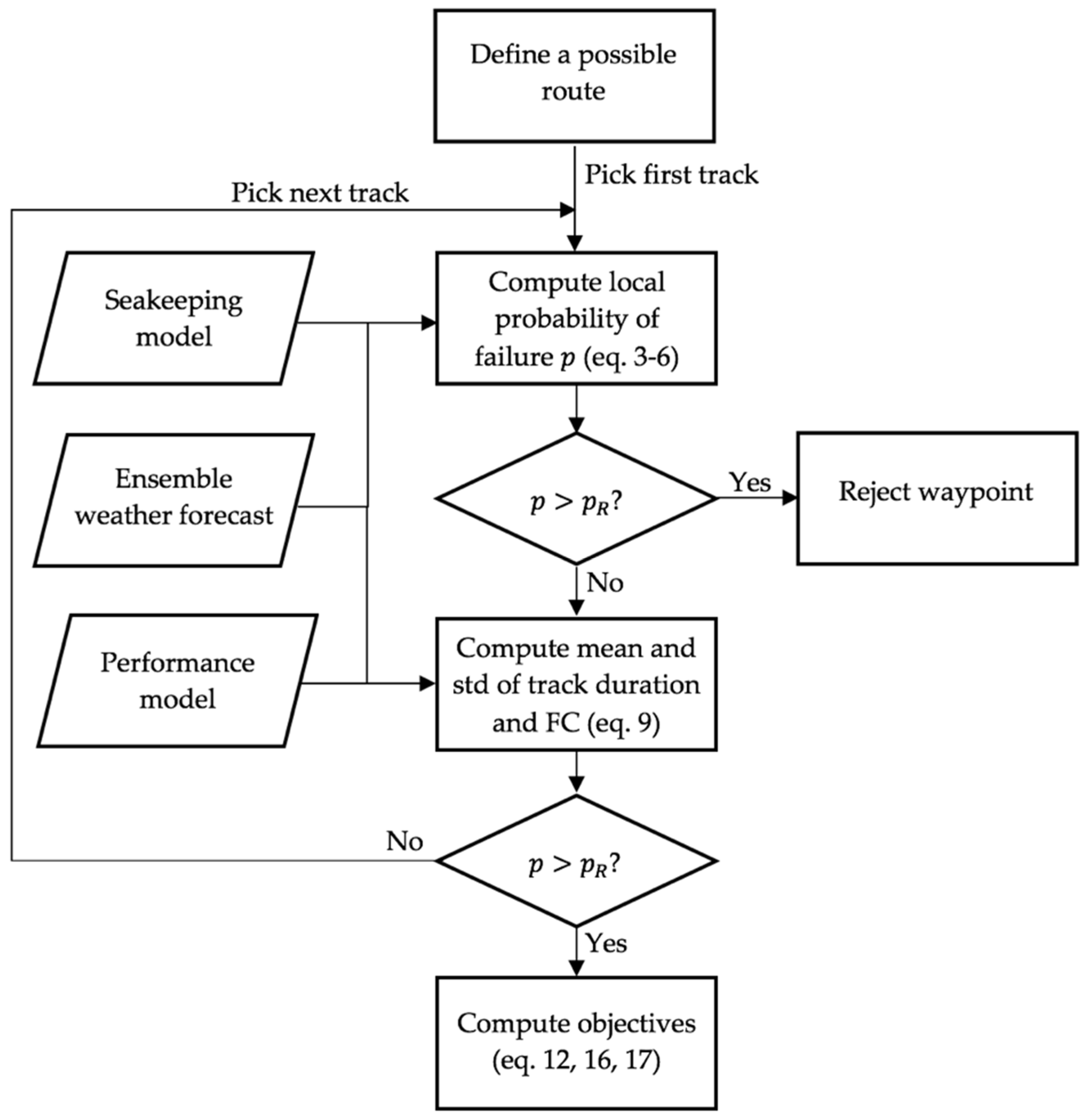
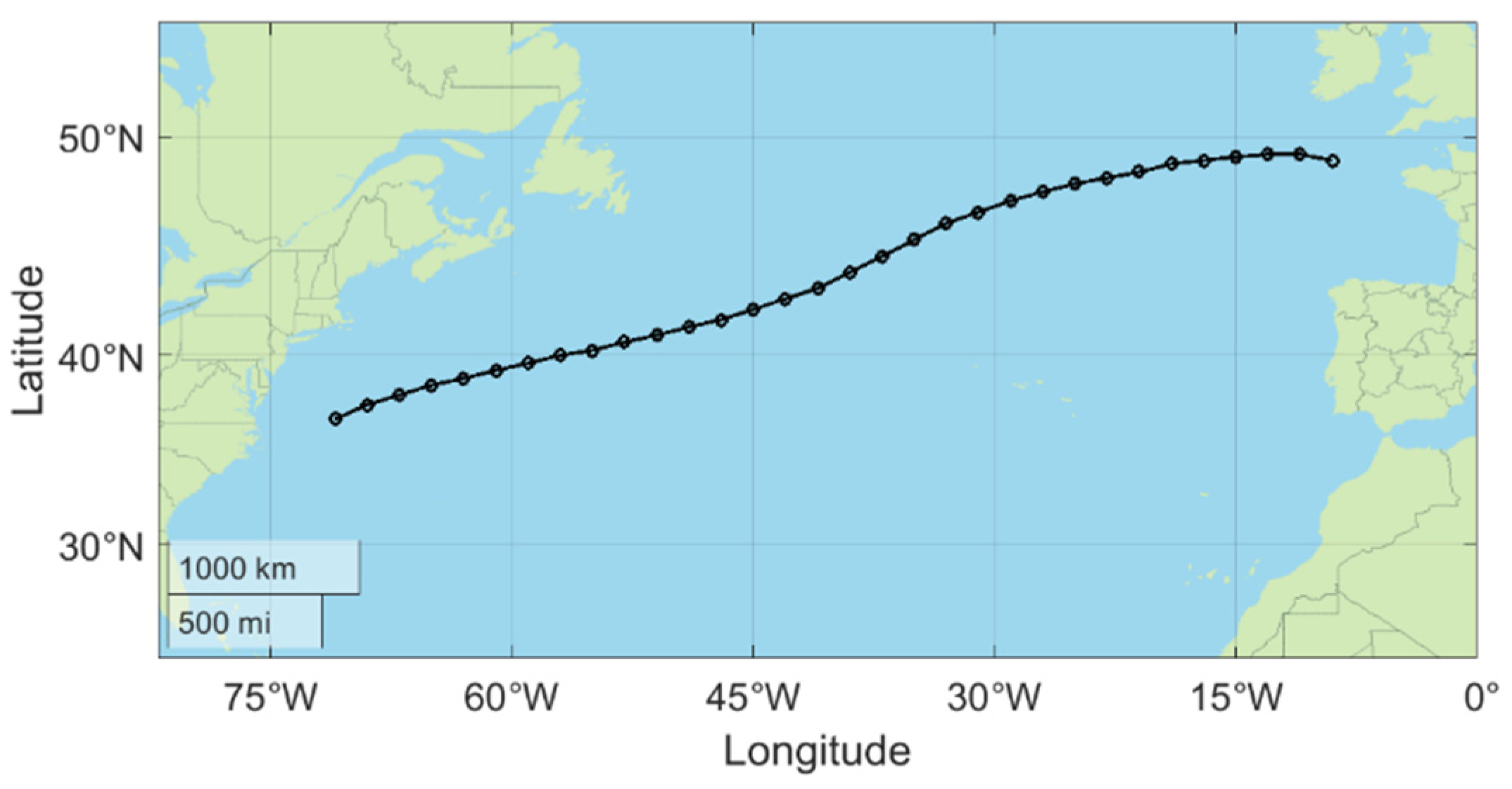
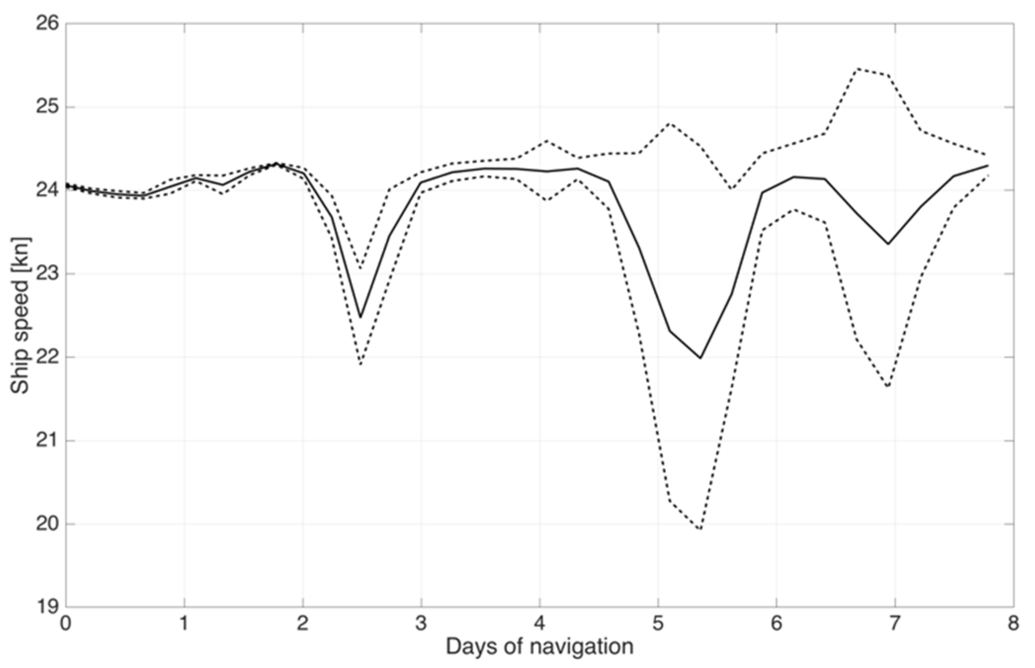
4. Example of Application

The process applied to implement the probabilistic approach discussed in the previous sections for the evaluation of route optimization constraints and objective functions is summarised in the flowchart in Figure 2.

The method has been applied to a transatlantic route starting from the British Channel with its destination on the east coast of the United States, as shown in Figure 3, being one of the most travelled commercial routes in this area [30].

The route simulation is made considering a containership with main characteristics listed in

Table 1. Main characteristics of the ship considered in the simulation.

$L_{pp}$	175.0	m
$B$	25.4	m
$T$	9.0	m
$\Delta$	22,775	t
Engine MCR	28,864	kW
Prop. diameter	6.33	m

.

The departure time is at midnight on 25 April 2020 and the engine is set to operate at $90\%$ of the maximum speed, corresponding to 129.6 RPM and a cruise speed of $24.35 \mathrm{kn}$ in still water. During the navigation, a constant RPM engine strategy is adopted [20] until the engine overload curve is reached; when the resistance increases, the RPMs are progressively reduced to prevent overloading and make the engine operate within acceptable working conditions according to the load diagram provided by the manufacturer.

The mean weather conditions expected along the route and the relative uncertainties are obtained from the NOAA GWES ensemble forecast [9], assuming the ship will travel at the speed corresponding to the mean weather conditions [31]. Figure 4 describes the significant wave height and the mean period forecasted during the navigation, including all the ensemble members, and highlighting the mean values and 5th and 95th percentiles; the encountered conditions are also depicted with dots.

It can be noticed that the initial part of the route is subjected to milder weather conditions, characterized by relatively low swells, and agreement among the ensembles due to the short prediction range. After two days, an area of moderate waves is expected with maximum $H_S$ reaching 4 m, though maintaining small variability among the members. In the second half of the voyage, the situation becomes more uncertain due to the long prediction range (>4 days) with some ensemble members showing values of $H_S$ close to 6 m. Indeed, these pessimistic predictions are those which more closely represent the actual sea-states encountered by the ship. Moreover, the significant wave height is always within the 90% confidence level, while the wave period exceeds the upper limit in some cases.

By applying the equations described in the previous sections based on the first-order second-moment method, the uncertainties in the weather prediction have been propagated in the model to estimate the uncertainties in the ship’s operational characteristics.

As shown in Figure 5, the variability of the speed is limited, with an average value always higher than 22 kn. This is due to a sufficient sea margin of the engine and the fact that the limits of the seakeeping responses are not exceeded, thus not requiring voluntary speed reduction [32].

On the other hand, Figure 6 indicates a large variability in the estimation of the fuel consumption, in this case represented in the form of fuel consumption per nautical mile. This is mostly explained by an increase in the power required to face the increased resistance due to more severe weather conditions, and the consequent decrease in speed [33].

The estimated value of the voyage fuel consumption, roughly corresponding to the only result that could be obtained with a deterministic approach, is equal to $408.7 \mathrm{t}$, while the $95{\mathrm{th}}^{}$ percentile is $418.4 \mathrm{t}$.

For what concerns safety, several seakeeping responses are taken into account, namely vertical acceleration at the bridge, lateral acceleration at a critical cargo location, roll, green water, and slamming, and the overall probability of failure is taken as the upper bound of Equation (12). The probabilities of failure computed with the four methods described in Section 3.2 are compared in

Table 2. Comparison of risk objective function computed with different methods.

$ris{k}_1$	$2.66\times {10}^{-5}$
$ris{k}_2$	$1.45\times {10}^{-6}$
$ris{k}_3$	$1.40\times {10}^{-5}$
$ris{k}_4$	$4.23\times {10}^{-6}$

.

The probabilities of failure are small in all cases, since no extreme conditions that could put the ship at risk are encountered in this voyage. However, the strength of the approach can be better estimated when used to rank different routes, as it provides a meaningful way to aggregate navigation hazards and to evaluate the probability of the severity of the entire voyage, accounting for uncertainties in the weather forecast.

5. Conclusions

A method has been proposed to exploit the additional information provided by ensemble weather forecasts in the identification of the most favourable ship route. Several assumptions are adopted with respect to the distribution of such uncertainties and their propagation in the model. Nevertheless, the method proposed has the advantage of being simple to adopt also on existing routing software, as it maintains the typical structures of objectives and constraints, extending the amount of information provided to the ranking method (and to the decision-maker) for a more aware selection. Prediction of route performance, identified with fuel consumption and duration of the voyage, are accompanied by the variance of such objectives, enabling the evaluation of the related percentiles, e.g., instead of a deterministic estimated time of arrival (ETA), the time within which the ship will arrive with 90% of probability can be considered. Navigation safety, which typically generates difficulties in the aggregation of different hazards, is consistently represented by the probability of system failure, which is the probability of exceeding predetermined thresholds of all the considered hazards. The test case provides a numerical example of the application of the method, highlighting the differences with a classical deterministic approach.

Further investigation will allow better appreciation of the strength of the proposed approach in the ranking of different routes and compare the accuracy of the predictions. Moreover, research is being conducted within the scope of the ROUTING project (http://routing-project.eu/ (accessed on 1 December 2021)) [34], aimed at obtaining the feedback of experienced seafarers that will support the tuning of specific parameters, such as the duration of severe conditions to compromise comfort and/or safety onboard and the percentiles of the expected ship performance, to achieve trustworthy predictions without assuming a too-conservative approach.

References

1. James, R. Application of Wave Forecasts to Marine Navigation; U.S. Naval Oceanographic Office: Washington, DC, USA, 1957.
2. Zis, T.P.V.; Psaraftis, H.N.; Ding, L. Ship weather routing: A taxonomy and survey. Ocean Eng. 2020, 213, 107697. [Google Scholar] [CrossRef]
3. Perera, L.P.; Guedes Soares, C. Weather routing and safe ship handling in the future of shipping. Ocean Eng. 2017, 130, 684–695. [Google Scholar] [CrossRef]
4. Vettor, R.; Guedes Soares, C. Multi-objective Route Optimization for Onboard Decision Support System. In Information, Communication and Environment: Marine Navigation and Safety of Sea Transportation; Weintrit, A., Neumann, T., Eds.; Taylor & Francis Group: Leiden, The Netherlands, 2015; pp. 99–106. [Google Scholar]
5. Szlapczynska, J. Multiobjective Approach to Weather Routing. Trans. Nav. Int. J. Mar. Navig. Safe Sea Transp. 2007, 1, 273–278. [Google Scholar]
6. Zaccone, R.; Ottaviani, E.; Figari, M.; Altosole, M. Ship voyage optimization for safe and energy-efficient navigation: A dynamic programming approach. Ocean Eng. 2018, 153, 215–224. [Google Scholar] [CrossRef]
7. Slingo, J.; Palmer, T. Uncertainty in weather and climate prediction. Philos. Trans. R. Soc. A 2011, 369, 4751–4767. [Google Scholar] [CrossRef] [PubMed]
8. Vettor, R.; Prpić-Oršić, J.; Guedes Soares, C. Impact of Wind Loads on Long-term Fuel Consumption and Emissions. Brodogradnja 2018, 69, 15–28. [Google Scholar] [CrossRef]
9. Chen, H.S. Ensemble prediction of ocean waves at NCEP. In Proceedings of the 28th Ocean Engineering Conference, Taiwan, China, 8–11 June 2006; National Sun Yat-Sen University: Taiwan, China, 2006; pp. 25–37. [Google Scholar]
10. Haiden, T.; Janousek, M.; Vitart, F.; Ferranti, L.; Prates, F. Evaluation of ECMWF Forecasts, Including the 2019 Upgrade; European Centre for Medium Range Weather Forecasts: Reading, UK, 2019. [Google Scholar]
11. Campos, R.M.; Guedes Soares, C. Global assessments of surface winds and waves from an ensemble forecast system using satellite data. In Proceedings of the ASME 2019 38th International Conference on Ocean, Offshore and Arctic Engineering (OMAE 2019), ASME Paper OMAE2019-96627—V07BT06A015, Glasgow, UK, 9–14 June 2019. [Google Scholar]
12. Hinnenthal, J.; Saetra, O. Robust Pareto—Optimal routing of ships utilizing ensemble weather forecasts. In Maritime Transportation and Exploitation of Ocean and Coastal Resources; Guedes Soares, C., Garbatov, Y., Fonseca, N., Eds.; Taylor & Francis Group: London, UK, 2005; pp. 1045–1050. [Google Scholar]
13. Halvorsen-Weare, E.E.; Fagerholt, K.; Rönnqvist, M. Vessel routing and scheduling under uncertainty in the liquefied natural gas business. Comput. Ind. Eng. 2013, 64, 290–301. [Google Scholar] [CrossRef] [Green Version]
14. Norlund, E.K.; Gribkovskaia, I. Environmental performance of speed optimization strategies in offshore supply vessel planning under weather uncertainty. Transp. Res. Part D 2017, 57, 10–22. [Google Scholar] [CrossRef]
15. Yoo, B.; Kim, J. Ship route optimization considering on-time arrival probability under environmental uncertainty. In Proceedings of the 2018 Ocean—MTS/IEEE Kobe Techno-Oceans, Kobe, Japan, 28–31 May 2018; pp. 1–5. [Google Scholar]
16. Vettor, R.; Guedes Soares, C. Reflecting the uncertainties of ensemble weather forecasts on the predictions of ship fuel consumption. Ocean Eng. 2021. Submitted for publication. [Google Scholar]
17. Manderbacka, T. On the uncertainties of the weather routing and support system against dangerous conditions. In Proceedings of the 17th International Ship Stability Workshop, Helsinki, Finland, 10–12 June 2019; pp. 10–12. [Google Scholar]
18. Guedes Soares, C. Effect of transfer function uncertainty on short-term ship responses. Ocean Eng. 1991, 18, 329–362. [Google Scholar] [CrossRef]
19. Guedes Soares, C.; Trovão, M.F.S. Sensitivity of Ship Motion Predictions to Wave Climate Descriptions. Int. Shipbuild. Prog. 1992, 39, 135–155. [Google Scholar]
20. Vettor, R.; Tadros, M.; Ventura, M.; Guedes Soares, C. Influence of main engine control strategies on fuel consumption and emissions. In Progress in Maritime Engineering and Technology; Guedes Soares, C., Santos, T.A., Eds.; Taylor & Francis Group: London, UK, 2018; pp. 157–163. ISBN 9780429505294. [Google Scholar]
21. Guedes Soares, C. Effect of Heavy Weather Maneuvering on the Wave-Induced Vertical Bending Moments in Ship Structures. J. Ship Res. 1990, 34, 60–68. [Google Scholar] [CrossRef]
22. Guedes Soares, C.; Fonseca, N.; Ramos, J. Prediction of Voyage Duration with Weather Constraints. In Proceedings of the International Conference on Ship Motions and Manoeuvrability, Royal Institute of Naval Architects, London, UK, 20 February 1998; pp. 1–13. [Google Scholar]
23. Fonseca, N.; Guedes Soares, C. Sensitivity of the Expected Ships Availability to Different Seakeeping Criteria. In Proceedings of the 21st International Conference on Offshore Mechanics and Arctic Engineering (Volume 4), Oslo, Norway, 23–28 June 2002; ASME Paper OMAE2002-28542. pp. 23–28. [Google Scholar]
24. Fonseca, N.; Guedes Soares, C. Experimental Investigation of the Shipping of Water on the Bow of a Containership. J. Offshore Mech. Arct. Eng. 2005, 127, 322–330. [Google Scholar] [CrossRef]
25. Melchers, R.E.; Beck, A.T. Structural Reliability Analysis and Prediction, 3rd ed.; John Wiley & Sons: Hoboken, NJ, USA, 2018. [Google Scholar]
26. Comstock, E.M.; Bales, S.L.; Keane, R.G. Seakeeping in ship operations. In Proceedings of the SNAME Ship Technology and Research Symposium, SanDiego, CA, USA, 3–7 June 1980. [Google Scholar]
27. Moreira, L.; Vettor, R.; Guedes Soares, C. Neural Network Approach for Predicting Ship Speed and Fuel Consumption. J. Mar. Sci. Eng. 2021, 9, 119. [Google Scholar] [CrossRef]
28. Vettor, R.; Guedes Soares, C. Analysis of the sensitivity of a multi-objective genetic algorithm for route optimization to different settings. In Maritime Technology and Engineering 3; Guedes Soares, C., Santos, T.A., Eds.; Taylor & Francis Group: London, UK, 2016; pp. 175–181. ISBN 9781138030008. [Google Scholar]
29. Rosa, G.J.; Wang, S.; Guedes Soares, C. Improvement of ship hulls for comfort in passenger vessels. In Developments in Maritime Technology and Engineering; Guedes Soares, C., Santos, T., Eds.; Taylor & Francis Group: London, UK, 2021; Volume 2, pp. 283–296. [Google Scholar]
30. Vettor, R.; Guedes Soares, C. Detection and analysis of the main routes of voluntary observing ships in the North Atlantic. J. Navig. 2015, 68, 397–410. [Google Scholar] [CrossRef] [Green Version]
31. Krata, P.; Vettor, R.; Guedes Soares, C. Bayesian approach to ship speed prediction based on operational data. In Developments in the Collision and Grounding of Ships and Offshore Structures; Guedes Soares, C., Ed.; Taylor & Francis Group: London, UK, 2020; pp. 384–390. [Google Scholar]
32. Vettor, R.; Guedes Soares, C. Rough weather avoidance effect on the wave climate experienced by oceangoing vessels. Appl. Ocean Res. 2016, 59, 606–615. [Google Scholar] [CrossRef]
33. Prpić-Oršić, J.; Vettor, R.; Faltinsen, O.M.; Guedes Soares, C. The influence of route choice and operating conditions on fuel consumption and CO2 emission of ships. J. Mar. Sci. Technol. 2016, 21, 434–445. [Google Scholar] [CrossRef] [Green Version]
34. Vettor, R.; Szlapczynska, J.; Szlapczynski, R.; Tycholiz, W.; Guedes Soares, C. Towards improving optimised ship weather routing. Polish Marit. Res. 2020, 27, 60–69. [Google Scholar] [CrossRef]
Figure 1. Representation of two constraints with the same average value and different uncertainties.
Jmse 09 01434 g001
Figure 2. Flowchart of the calculation process.
Jmse 09 01434 g002
Figure 3. Path of the considered route.
Jmse 09 01434 g003
Figure 4. Ensemble forecasts of H S (a) and T m (b) along the route: ensemble members, thin grey lines; mean of the ensembles, thick black line; 5th and 95th percentiles, dashed lines; actual weather occurred, dots.
Jmse 09 01434 g004
Figure 5. Evolution of mean value of V S and 90 % confidence interval along the route applying the first-order second-moment method.
Jmse 09 01434 g005
Figure 6. Evolution of mean value of F C n m i and 90 % confidence interval along the route applying the first-order second-moment method.
Jmse 09 01434 g006