Figure 1.
CALM buoy in Lazy-S configuration depicting offloading and loading operation.
Figure 1.
CALM buoy in Lazy-S configuration depicting offloading and loading operation.
Figure 2.
CALM Buoy with an FSO offloading tanker off the shore of Sudan (Courtesy of Bluewater).
Figure 2.
CALM Buoy with an FSO offloading tanker off the shore of Sudan (Courtesy of Bluewater).
Figure 3.
An illustration showing (a) displaced hose-beam element showing moments and forces, and (b) Submarine hose segment showing spline line and nodes.
Figure 3.
An illustration showing (a) displaced hose-beam element showing moments and forces, and (b) Submarine hose segment showing spline line and nodes.
Figure 4.
Buoy Design in ANSYS AQWA 2020 R2 showing (a) Hydrodynamic Panel, and (b) Wave Direction on buoy.
Figure 4.
Buoy Design in ANSYS AQWA 2020 R2 showing (a) Hydrodynamic Panel, and (b) Wave Direction on buoy.
Figure 5.
CALM Buoy Model showing (a) shaded view, and (b) wireframe view, modelled in Orcaflex 11.
Figure 5.
CALM Buoy Model showing (a) shaded view, and (b) wireframe view, modelled in Orcaflex 11.
Figure 6.
Schematic of marine hoses attached to a floating buoy in Lazy-S config. (Author, but Hose Courtesy: EMSTEC).
Figure 6.
Schematic of marine hoses attached to a floating buoy in Lazy-S config. (Author, but Hose Courtesy: EMSTEC).
Figure 7.
Numerical hose model in Orcaflex 11.0 f showing (a) CALM Buoy Lazy-S configuration showing mooring lines and submarine hoses, and (b) Submarine Hose Profile showing the radii for inner and outer surfaces.
Figure 7.
Numerical hose model in Orcaflex 11.0 f showing (a) CALM Buoy Lazy-S configuration showing mooring lines and submarine hoses, and (b) Submarine Hose Profile showing the radii for inner and outer surfaces.
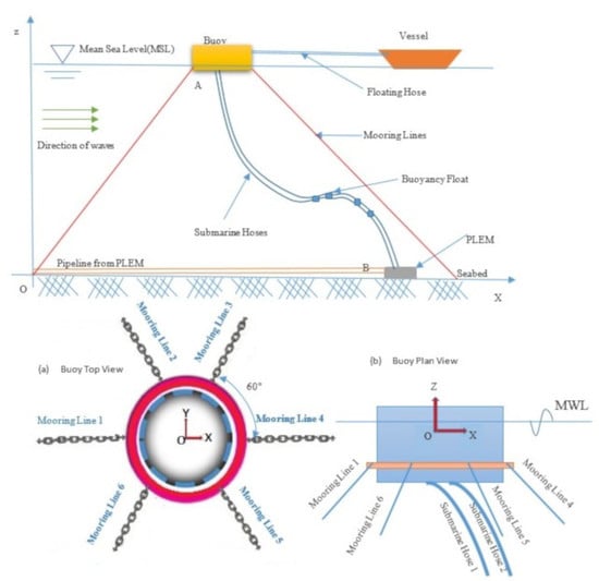
Figure 8.
The Cartesian Coordinate System showing the Buoy and Mooring Lines in (a) top view (b) side view.
Figure 8.
The Cartesian Coordinate System showing the Buoy and Mooring Lines in (a) top view (b) side view.
Figure 9.
Typical floats attached to offshore submarine hoses.
Figure 9.
Typical floats attached to offshore submarine hoses.
Figure 10.
Orcaflex Line Model showing (
a) the main line, (
b) the discretized model, (
c) Detailed model representation with 3 spring-damper types (Adapted, courtesy of Orcina [
73]).
Figure 10.
Orcaflex Line Model showing (
a) the main line, (
b) the discretized model, (
c) Detailed model representation with 3 spring-damper types (Adapted, courtesy of Orcina [
73]).
Figure 11.
CALM Buoy system finite element model showing Orcaflex details of (a) FEM wireframe view (b) nodal axes (c) buoy and mooring line nodes (d) submarine hoses with floats.
Figure 11.
CALM Buoy system finite element model showing Orcaflex details of (a) FEM wireframe view (b) nodal axes (c) buoy and mooring line nodes (d) submarine hoses with floats.
Figure 12.
Soil model characteristics showing different modes (Adapted, courtesy of Orcina [
73]).
Figure 12.
Soil model characteristics showing different modes (Adapted, courtesy of Orcina [
73]).
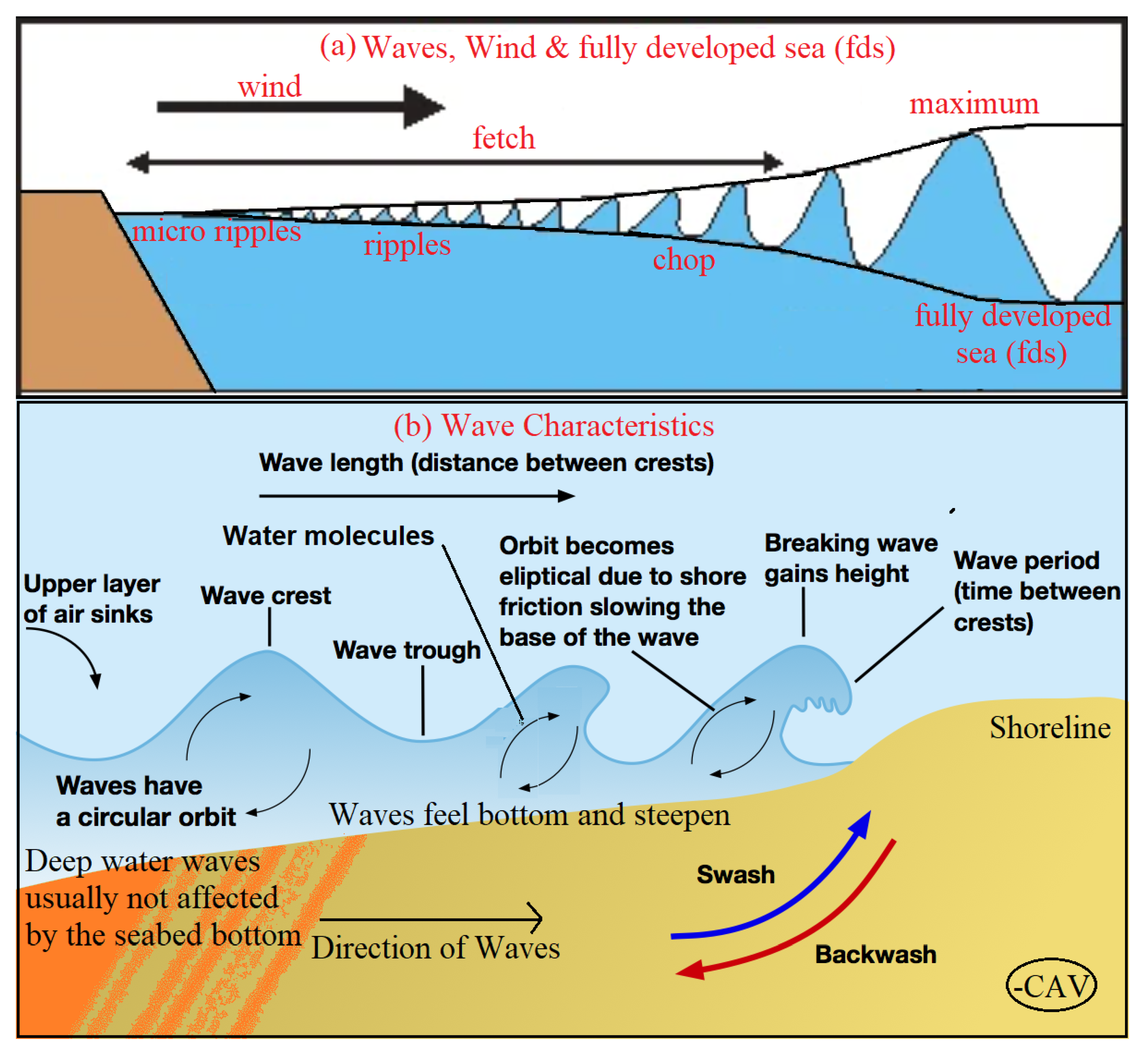
Figure 13.
Illustration of: (a) wind, waves and Fully Developed Sea (fds) profiles, and (b) wave characteristics.
Figure 13.
Illustration of: (a) wind, waves and Fully Developed Sea (fds) profiles, and (b) wave characteristics.
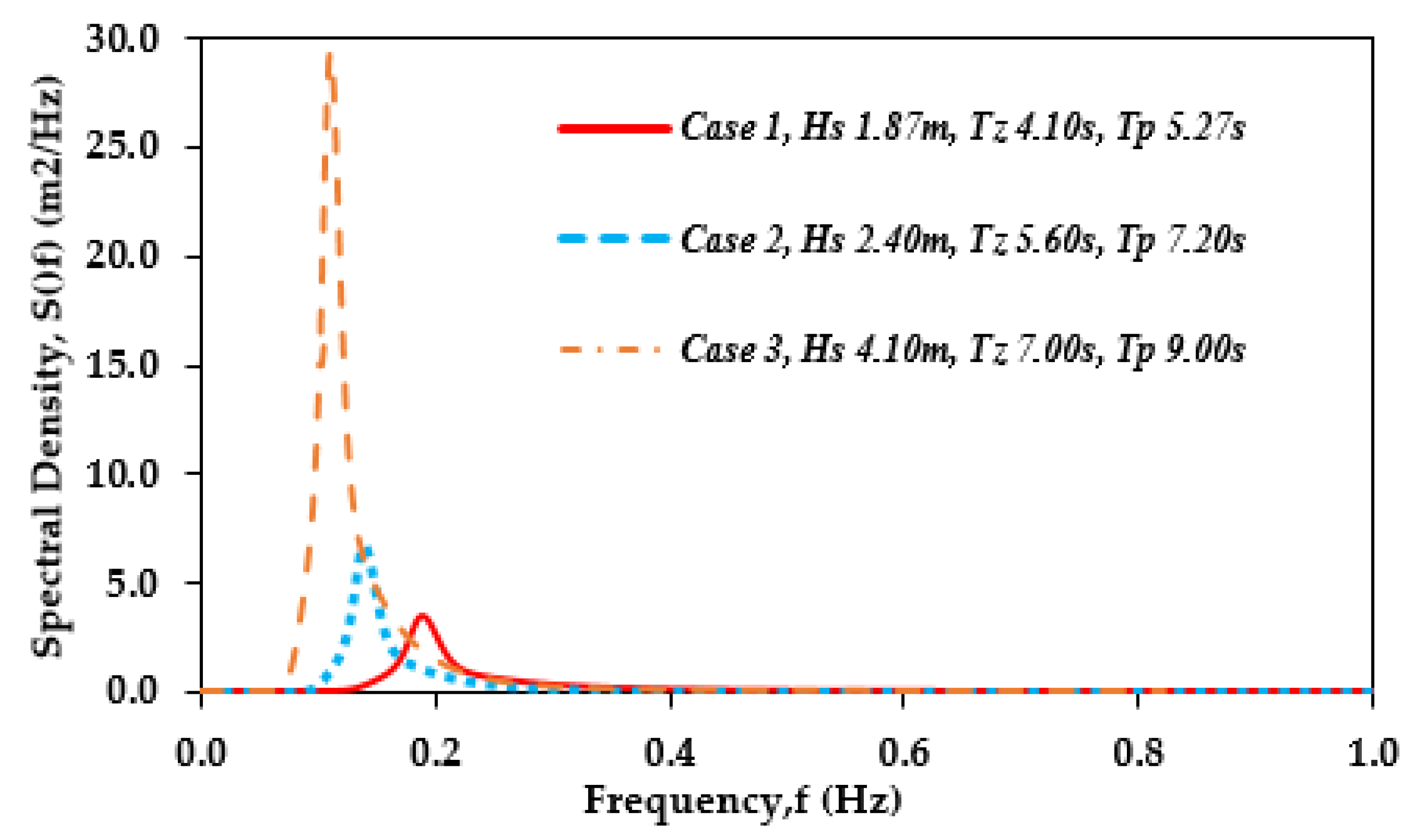
Figure 14.
JONSWAP Spectrum for the 3 Sea States or Environmental Cases.
Figure 14.
JONSWAP Spectrum for the 3 Sea States or Environmental Cases.
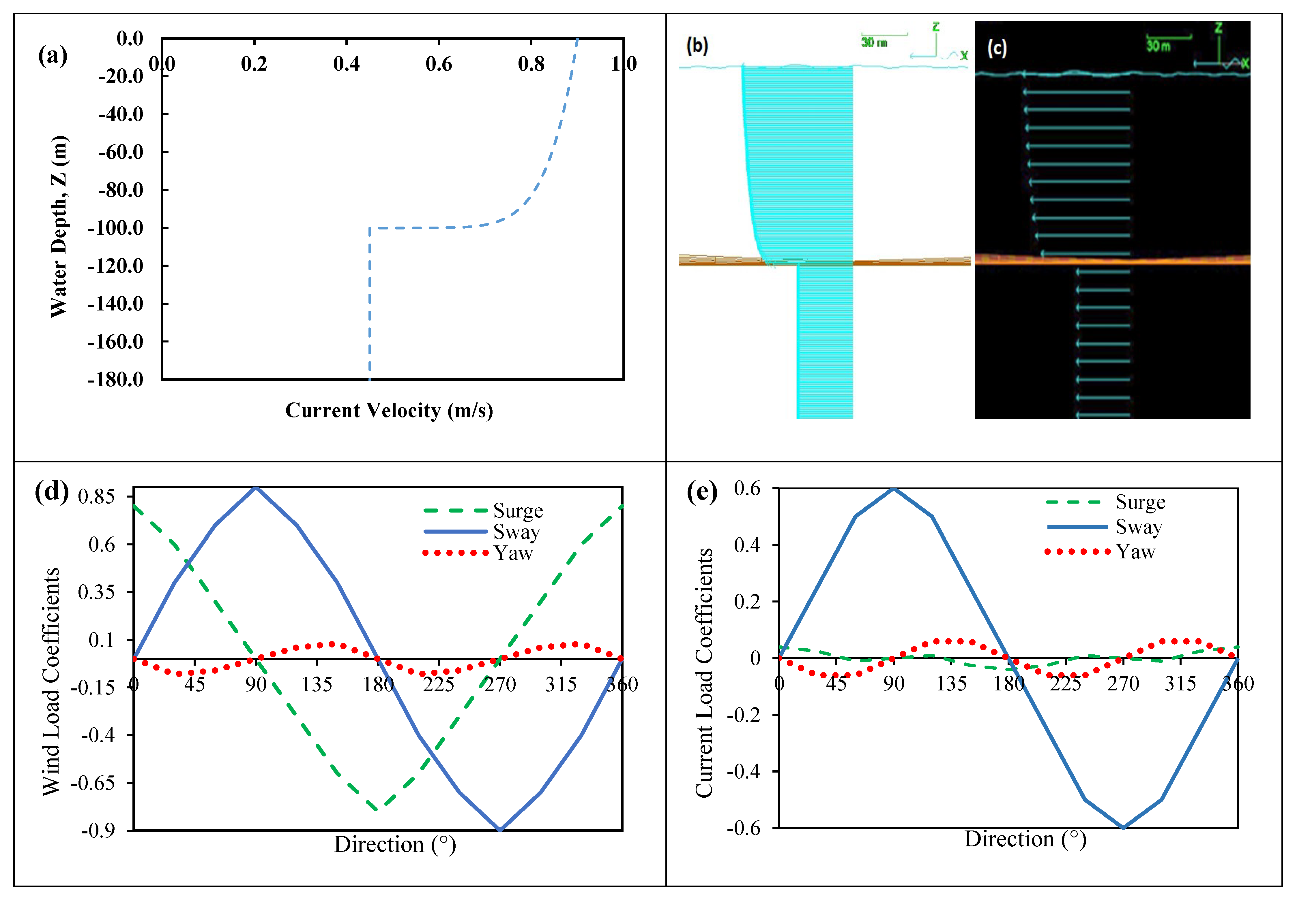
Figure 15.
Profiles showing details of (a) the vertical profile for Surface Current and Seabed Current at seabed origin, and (b) the Orcaflex 3D current profile for both currents, (c) the Orcaflex 2D current profile for both currents, (d) Load Coefficient for Wind on the CALM buoy, and (e) Load Coefficient for Current on the CALM buoy.
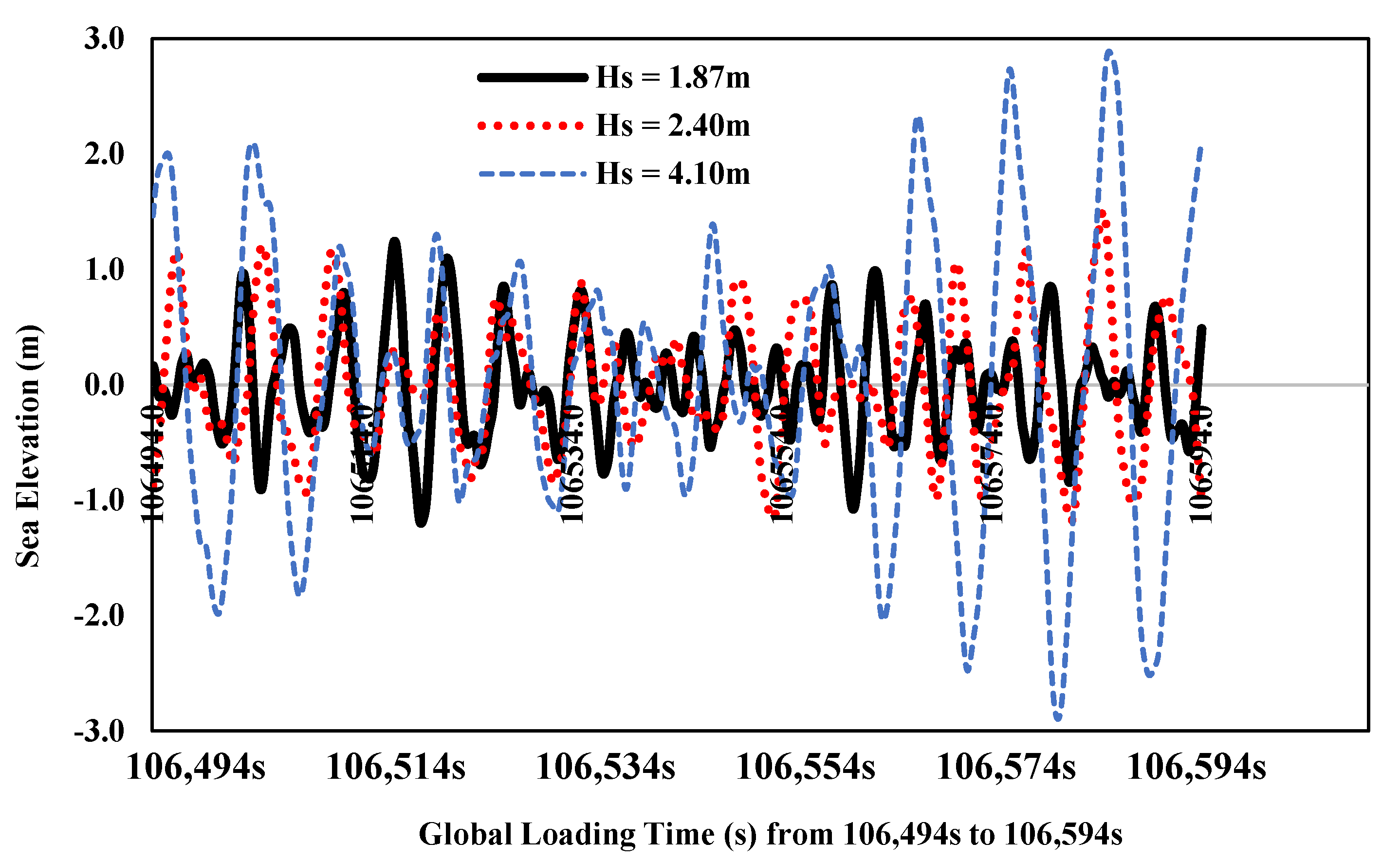
Figure 16.
Wave Loading Time History for the 3 Environmental Cases.
Figure 16.
Wave Loading Time History for the 3 Environmental Cases.
Figure 17.
Schematic of Catenary Mooring system of CALM Buoy.
Figure 17.
Schematic of Catenary Mooring system of CALM Buoy.
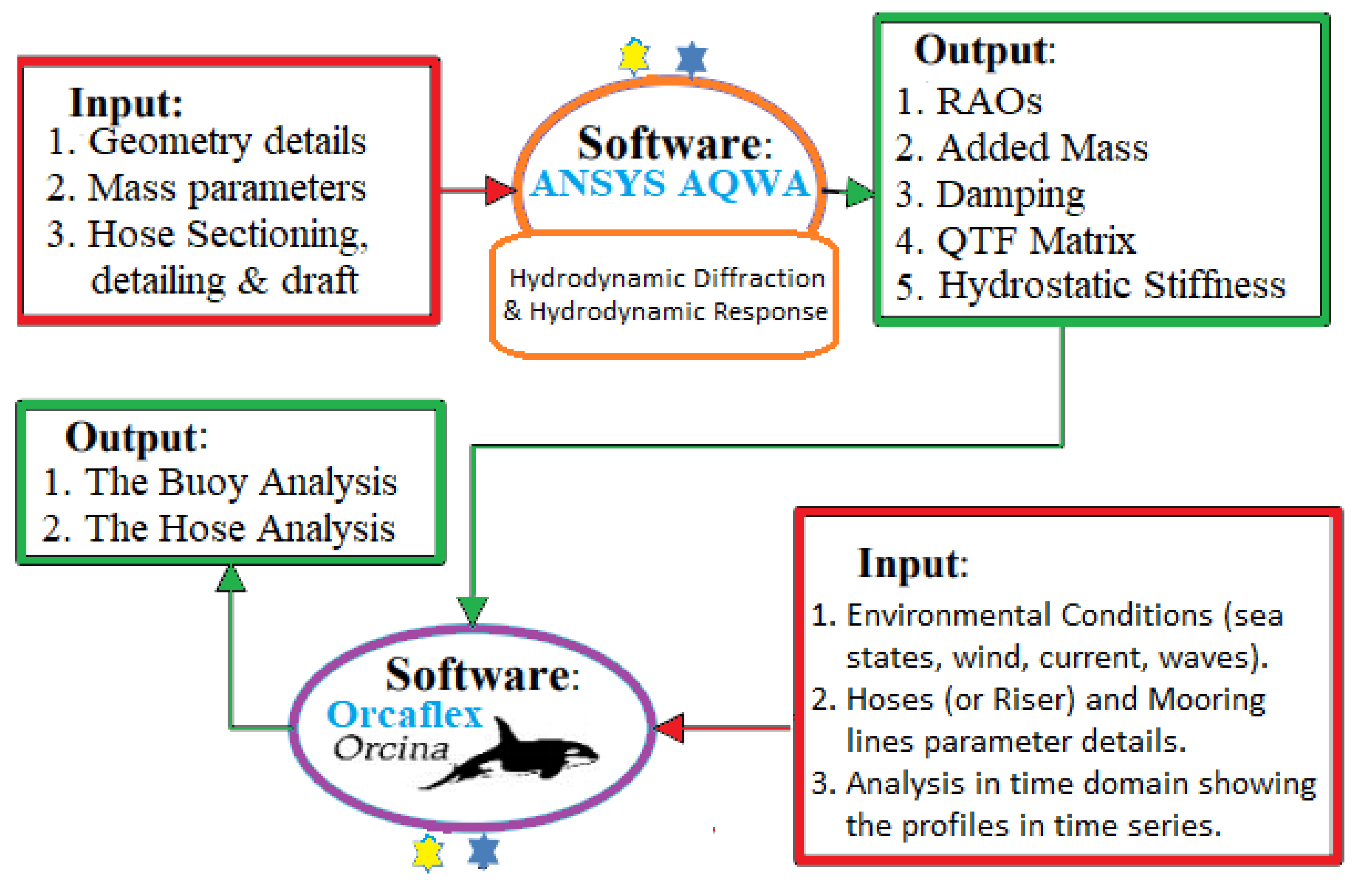
Figure 18.
Flow diagram of the methodology for the design analysis.
Figure 18.
Flow diagram of the methodology for the design analysis.
Figure 19.
Definition of sea flow angles in approach direction relative to FPSO, showing (a) waves on FPSO and (b) the wave heading with other different types of seas defined.
Figure 19.
Definition of sea flow angles in approach direction relative to FPSO, showing (a) waves on FPSO and (b) the wave heading with other different types of seas defined.
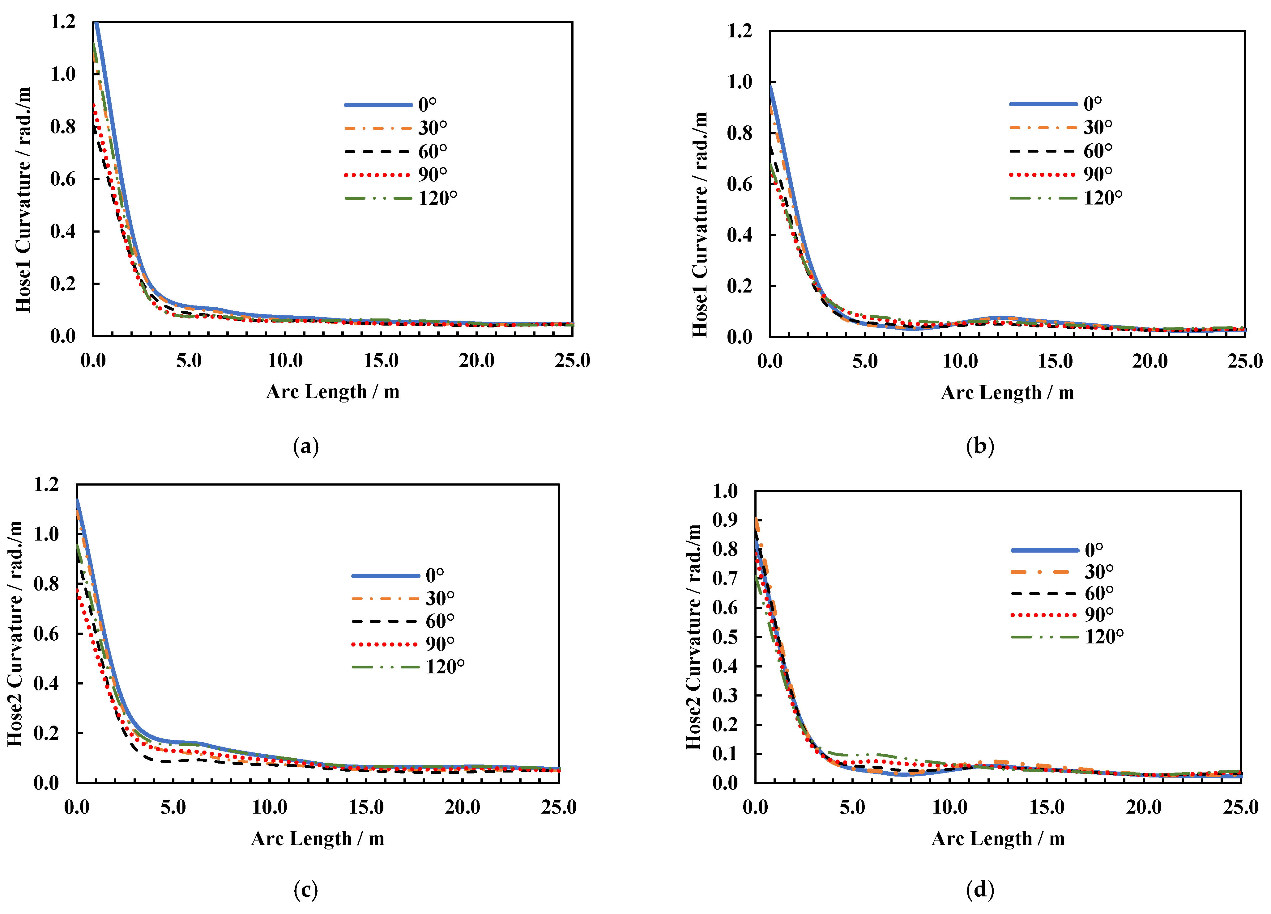
Figure 20.
Influence of RAOs for different environmental cases on hose curvature. Figure (a,c) are when the hoses have RAO loads, while Figure (b,d) are when the hoses are without RAO loads for the submarine hoses in Lazy-S config. (a) Hose1 Curvature including hose hydrodynamic load. (b) Hose1 Curvature excluding hose hydrodynamic load.(c) Hose2 Curvature including hose hydrodynamic load. (d) Hose2 Curvature excluding hose hydrodynamic load.
Figure 21.
Influence of RAOs on curvature for different wave directions. Figure (a,c) are when the hoses have RAO loads, while Figure (b,d) are when the hoses are without RAO loads for the submarine hoses in Lazy-S config. (a) Hose1 Curvature including hose hydrodynamic load. (b) Hose1 Curvature excluding hose hydrodynamic load. (c) Hose2 Curvature including hose hydrodynamic load. (d) Hose2 Curvature excluding hose hydrodynamic load.
Figure 22.
Influence of RAOs on effective tensions for different environmental cases. Figure (a,c) are when the hoses have RAO loads, while Figure (b,d) are when the hoses are without RAO loads for the submarine hoses in Lazy-S. (a) Hose1 Effective Tension including hose hydrodynamic load. (b) Hose1 Effective Tension excluding hose hydrodynamic load. (c) Hose2 Effective Tension including hose hydrodynamic load. (d) Hose2 Effective Tension excluding hose hydrodynamic load.
Figure 23.
Influence of RAOs on Effective Tension for different wave directions. Figure (a,c) are when the hoses have RAO loads, while Figure (b,d) are when the hoses are without RAO loads for the submarine hoses in Lazy-S config.(a) Hose1 Effective Tension including hose hydrodynamic load. (b) Hose1 Effective Tension excluding hose hydrodynamic load. (c) Hose2 Effective Tension including hose hydrodynamic load. (d) Hose2 Effective Tension excluding hose hydrodynamic load.
Figure 24.
Influence of RAOs on bending moments for different environmental cases. Figure (a,c) are when the hoses have RAO loads, while Figure (b,d) are when the hoses are without RAO loads for the submarine hoses in Lazy-S. (a) Hose1 Bending Moment including hose hydrodynamic load. (b) Hose1 Bending Moment excluding hose hydrodynamic load. (c) Hose2 Bending Moment including hose hydrodynamic load. (d) Hose2 Bending Moment excluding hose hydrodynamic load.
Figure 25.
Influence of RAOs on bending moments for different wave directions. Figure (a,c) are when the hoses have RAO loads, while Figure (b,d) are when the hoses are without RAO loads for the submarine hoses in Lazy-S config. (a) Hose1 Bending Moment including hose hydrodynamic load. (b) Hose1 Bending Moment excluding hose hydrodynamic load. (c) Hose2 Bending Moment including hose hydrodynamic load. (d) Hose2 Bending Moment excluding hose hydrodynamic load.
Figure 26.
Results on DAFHose for different environmental cases. Figure (a,c) are when the hoses have RAO loads, while Figure (b,d) are when the hoses are without RAO loads for the submarine hoses in Lazy-S config. (a) Bending Moment DAFHose for Hose1. (b) Bending Moment DAFHose for Hose2. (c) Effective Tension DAFHose for Hose1. (d) Effective Tension DAFHose for Hose2.
Figure 27.
Result of surface currents (a,b) and seabed currents (c,d) on submarine hoses. (a) Bending Moment for surface current on arc lengths. (b) Effective tension for surface current on arc lengths. (c) Bending Moment for seabed current on arc lengths. (d) Effective tension for seabed current on arc lengths.
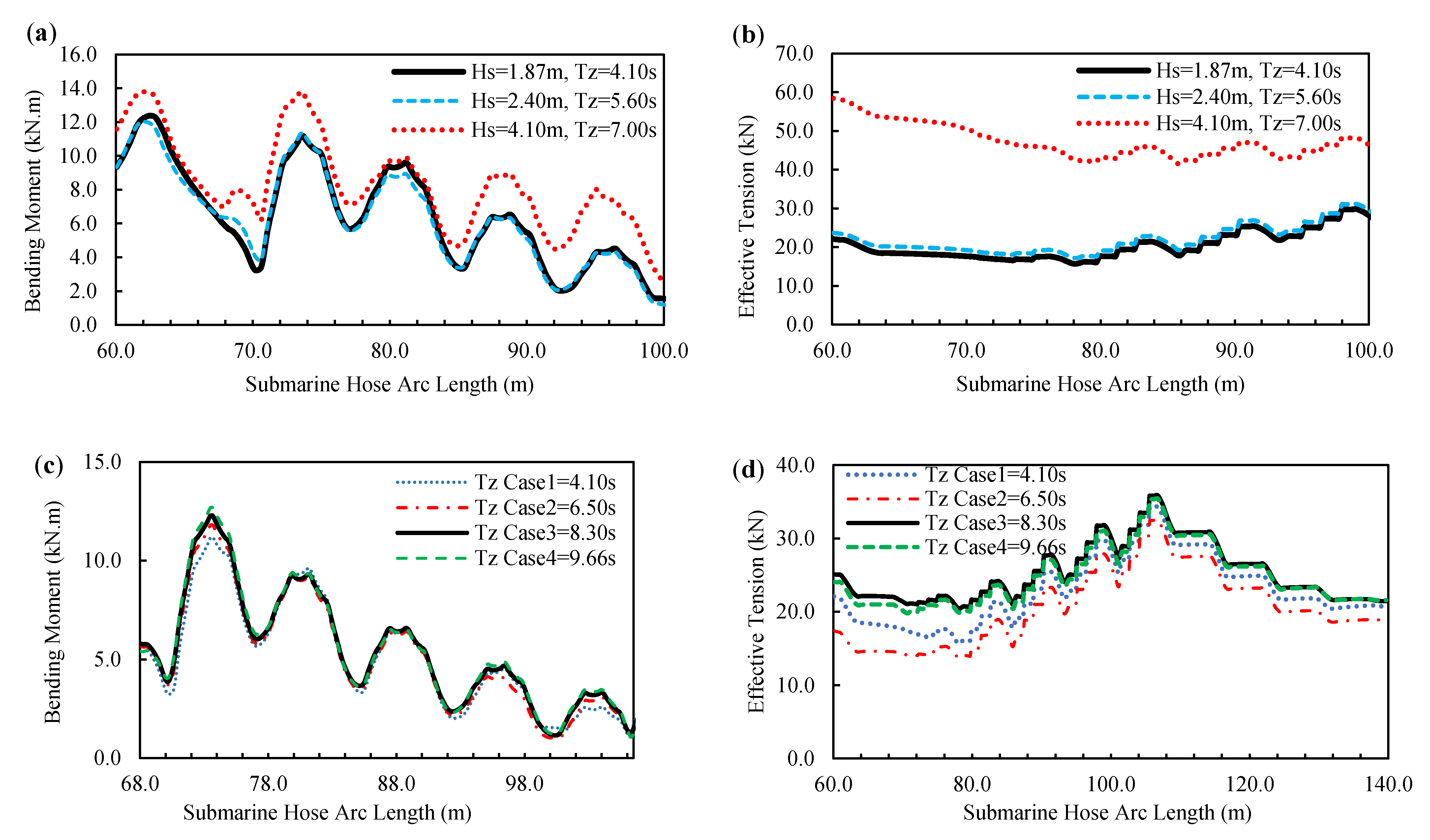
Figure 28.
Influence of surface wave direction for the submarine hoses. (a) Bending Moment for hose arc lengths 60–100 m. (b) Effective Tension for hose arc lengths 60–100 m.
Figure 28.
Influence of surface wave direction for the submarine hoses. (a) Bending Moment for hose arc lengths 60–100 m. (b) Effective Tension for hose arc lengths 60–100 m.
Figure 29.
Influence of environmental conditions on submarine hoses. (a) Bending Moment for load cases. (b) Effective tension for load cases. (c) Bending Moment for Tz. (d) Effective tension for Tz.
Figure 29.
Influence of environmental conditions on submarine hoses. (a) Bending Moment for load cases. (b) Effective tension for load cases. (c) Bending Moment for Tz. (d) Effective tension for Tz.
Figure 30.
Effect of Float outer diameter on the submarine hoses. (a) Bending Moment for hose arc lengths 60–140 m. (b) Effective Tension for hose arc lengths 60–140 m.
Figure 30.
Effect of Float outer diameter on the submarine hoses. (a) Bending Moment for hose arc lengths 60–140 m. (b) Effective Tension for hose arc lengths 60–140 m.
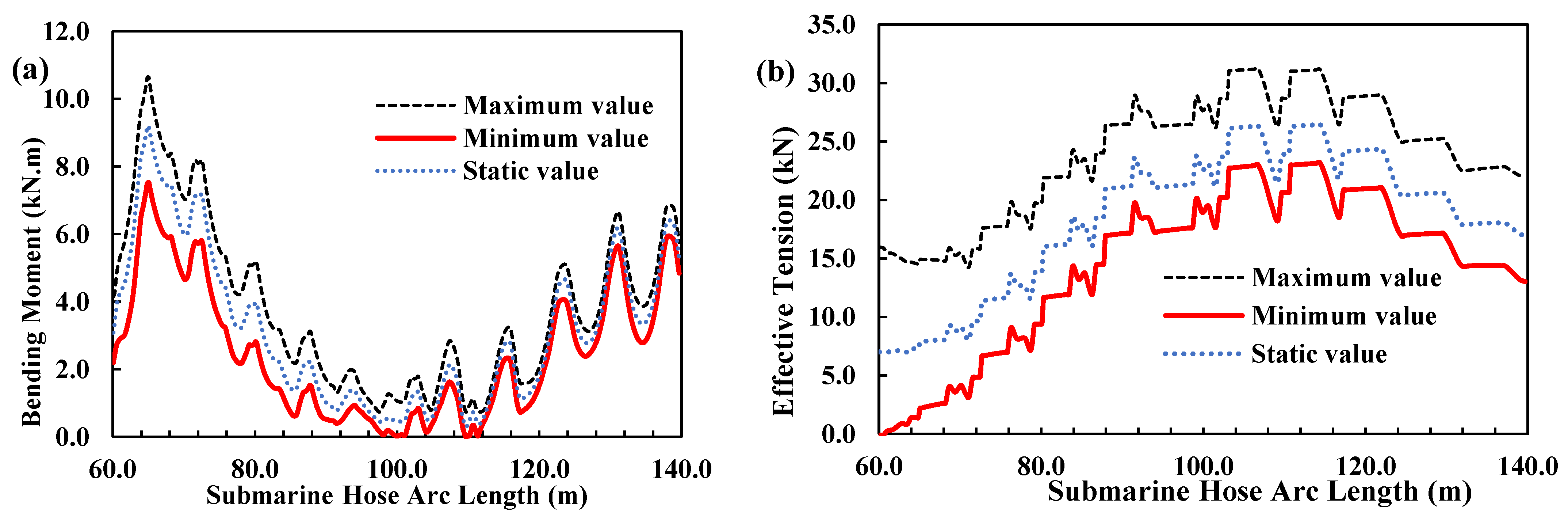
Figure 31.
Effect of hose segment lengths of submarine hoses. (a) Bending Moment for hose segment lengths. (b) Effective tension for hose segment lengths.
Figure 31.
Effect of hose segment lengths of submarine hoses. (a) Bending Moment for hose segment lengths. (b) Effective tension for hose segment lengths.
Figure 32.
Effect of float buoyancy length location along hose arc length.
Figure 32.
Effect of float buoyancy length location along hose arc length.
Figure 33.
Influence of Seabed Soil Model on the submarine hoses, for (a) Bending moment, (b) Effective Tension, (c) Seabed normal penetration/D, and (d) Seabed normal resistance.
Figure 33.
Influence of Seabed Soil Model on the submarine hoses, for (a) Bending moment, (b) Effective Tension, (c) Seabed normal penetration/D, and (d) Seabed normal resistance.
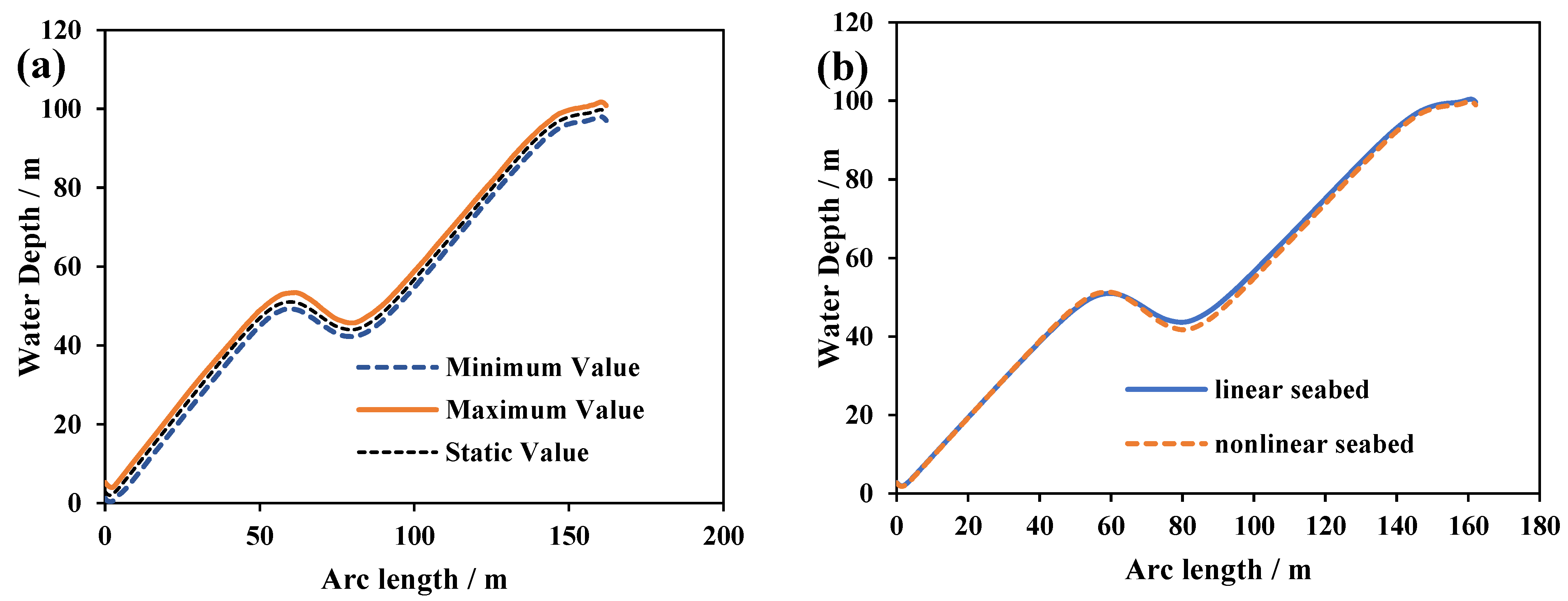
Figure 34.
Influence of water depth and hose static offset in Lazy-S configuration on submarine hoses. (a) Effect of water depth on static offset configuration of lazy-S hoses for linear seabed. (b) Effect of water depth on static offset for linear and non-linear seabeds.
Figure 34.
Influence of water depth and hose static offset in Lazy-S configuration on submarine hoses. (a) Effect of water depth on static offset configuration of lazy-S hoses for linear seabed. (b) Effect of water depth on static offset for linear and non-linear seabeds.
Figure 35.
Influence of soil shear strength gradient and soil stiffness on submarine hoses. (a) Bending Moment for soil shear strength gradient. (b) Effective tension for soil shear strength gradient. (c) Bending Moment for soil stiffness. (d) Effective tension for soil stiffness.
Figure 35.
Influence of soil shear strength gradient and soil stiffness on submarine hoses. (a) Bending Moment for soil shear strength gradient. (b) Effective tension for soil shear strength gradient. (c) Bending Moment for soil stiffness. (d) Effective tension for soil stiffness.
Table 1.
Parameters for the Buoy.
Table 1.
Parameters for the Buoy.
| Particulars | Value |
|---|
| Buoy Height (m) | 4.40 |
| Draft size (m) | 2.40 |
| Water Depth (m) | 100.00 |
| Buoy Mass (kg) | 198,762.00 |
| Main body diameter (m) | 10.00 |
| Skirt diameter (m) | 13.87 |
Table 2.
Submarine Hose Arrangement with section details.
Table 2.
Submarine Hose Arrangement with section details.
| Section Number | Sub-Sections | Particulars | Inner Diameter (m) | Outer Diameter (m) | Section Length (m) | Segment Length (m) | Number of Segments | Unit Mass (kg/m) | Volume (m3) | Segment Weight (N) |
|---|
| Hose Group 1—Section 1 | 1 | Fitting | 0.489 | 0.650 | 1.0 | 0.800 | 1 | 495 | 0.330 | 492.5 |
| 2 | Reinforced Hose End | 0.489 | 0.650 | 0.2 | 3.000 | 15 | 239 | 1.002 | 721.5 |
| 3 | Hose Body | 0.489 | 0.650 | 0.5 | 3.236 | 6 | 180 | 1.074 | 582.5 |
| 4 | Hose End | 0.489 | 0.675 | 0.5 | 0.895 | 2 | 200 | 0.320 | 179.0 |
| 5 | Fitting | 0.489 | 0.650 | 1.0 | 0.800 | 1 | 495 | 0.330 | 492.5 |
| Hose Group 2—Section 2—Section 20 (same) | 6 | Fitting | 0.489 | 0.650 | 1.0 | 0.800 | 1 | 495 | 0.330 | 492.5 |
| 7 | Hose End | 0.489 | 0.675 | 0.5 | 0.895 | 2 | 200 | 0.320 | 179.0 |
| 8 | Hose Body | 0.489 | 0.650 | 0.2 | 3.840 | 19 | 180 | 1.274 | 691.2 |
| 9 | Hose End | 0.489 | 0.675 | 0.5 | 0.895 | 2 | 200 | 0.320 | 179.0 |
| 10 | Fitting | 0.489 | 0.650 | 1.0 | 0.800 | 1 | 495 | 0.330 | 492.5 |
| Hose Group 3—Section 21 | 11 | Fitting | 0.489 | 0.650 | 1.0 | 0.800 | 1 | 495 | 0.330 | 492.5 |
| 12 | Hose End | 0.489 | 0.675 | 0.5 | 0.895 | 2 | 200 | 0.320 | 179.0 |
| 13 | Hose Body | 0.489 | 0.650 | 0.5 | 3.236 | 6 | 180 | 1.074 | 582.5 |
| 14 | Reinforced Hose End | 0.489 | 0.670 | 0.2 | 3.000 | 15 | 240 | 1.064 | 724.6 |
| 15 | Fitting | 0.489 | 0.650 | 1.0 | 0.800 | 1 | 495 | 0.330 | 492.5 |
Table 3.
Mooring Lines Parameters.
Table 3.
Mooring Lines Parameters.
| Parameters | Value |
|---|
| Poisson Ratio | 0.5 |
| Nominal Diameter (m) | 0.120 |
| Ratio of Section Lengths | 150:195 |
| Mass per unit length (kg/m) | 0.088 |
| Coefficient of Drag, Cd | 1.0 |
| Coefficient of Mass, Cm | 1.0 |
| Bending Stiffness (N*m2) | 0.010 |
| Axial Stiffness, EA (kN) | 407,257 |
| Contact Diameter (m) | 0.229 |
Table 4.
Parameters of Buoyancy float.
Table 4.
Parameters of Buoyancy float.
| Parameters | Value |
|---|
| Pitch of Floats, Pf (m) | 2.00 (depends on section) |
| Weight in Air (kg) | 102.00 |
| Outer Diameter (m) | 1.23 |
| Net Buoyancy (kg) | 280.00 |
| Inner Diameter, Df (m) | 0.799 |
| Length of Float, Lf (m) | 0.60 |
| Design Depth (m) | 40 |
| Material for Shell | Polyethylene |
| Material for Filling | Polyurethane foam |
| Material for Metallic Sections | Stainless Steel |
| Float Classification | Standard bolted-type float |
Table 5.
Non-linear Soil Model parameters.
Table 5.
Non-linear Soil Model parameters.
| Parameter | Symbol | Value |
|---|
| Mudline Shear Strength (kPa) | Su0 | 4.5 |
| Shear Strength Gradient (kPa/m) | Sg | 1.5 |
| Saturated Soil Density (te/m3) | ρsoil | 1.5 |
| Power Law Parameter | a | 6.0 |
| Power Law Parameter | b | 0.25 |
| Soil Buoyancy Factor | fb | 1.5 |
| Normalized Maximum Stiffness (kNm−1m2) | Kmax | 200.0 |
| Suction Resistance Ratio | fsuc | 0.7 |
| Suction Decay Parameter | λsuc | 1.0 |
| Repenetration Parameter | λrep | 0.3 |
Table 6.
Seabed and Ocean Parameters.
Table 6.
Seabed and Ocean Parameters.
| Parameter | Value | Parameter | Value |
|---|
| Water Density (kgm−3) | 1,025 | Ocean Temperature (°C) | 10 |
| Ocean Kinematic Viscosity (m2s−1) | 1.35 × 10⁻⁶ | Water Depth (m) | 100.0 |
| Wave Amplitude (m) | 0.145 | Seabed Friction Coefficient | 0.5 |
| Seabed Stiffness (kNm−1m2) | 7.5 | Seabed Shape Direction (°) | 0 |
| Seabed Critical Damping (%) | 0 | Seabed Model Profile Type | 3D Profile Nonlinear |
Table 7.
Wave Parameters for the 3 load Cases.
Table 7.
Wave Parameters for the 3 load Cases.
| Case No. | HS (m) | TZ (s) | TP (s) |
|---|
| 1 | 1.87 | 4.10 | 5.27 |
| 2 | 2.40 | 5.60 | 7.20 |
| 3 | 4.10 | 7.00 | 9.00 |
Table 8.
Wind and Current Parameters.
Table 8.
Wind and Current Parameters.
| Parameter | Value |
|---|
| Wind Speed (ms−1) | 22.00 |
| Wind Type | Constant |
| Density of Air (gcm−3) | 0.001225 |
| Kinematic Viscosity of Air (m2s−1) | 0.000015 |
| Power Law Exponent | 7.00 |
| Current Method | Power Law |
| Current Direction (°) | 180 |
| Surface Current (ms−1) | 0.50 |
| Seabed Current (ms−1) | 0.45 |
Table 9.
Definition of Case Study for the 3 Environmental Cases.
Table 9.
Definition of Case Study for the 3 Environmental Cases.
| Case Study | Flow Angles (°) | Hydrodynamic Loads (HL) |
|---|
| 1 | 0,30,60,90,120 | Hose with HL, Hose without HL |
| 2 | 0,30,60,90,120 | Hose with HL, Hose without HL |
| 3 | 0,30,60,90,120 | Hose with HL, Hose without HL |
Table 10.
Parameters for Hydrodynamic Coefficients.
Table 10.
Parameters for Hydrodynamic Coefficients.
| Parameters | Value |
|---|
| Drag Coefficient, Cd | 0.7 |
| Inertia Coefficient, Cm | 2.0 |
| Added Mass Coefficient, Ca = Cm−1 | 1.0 |
| Normal Added Mass Force Coefficient | 0.7 |
| Axial Added Mass Force Coefficient | 1.1 |
Table 11.
Mesh Grid independence for Surge Study using diffraction analysis.
Table 11.
Mesh Grid independence for Surge Study using diffraction analysis.
| Size of Element (m) | Number of Nodes | Number of Elements | Max. Surge RAO (m/m) | Max. RAO Deviation on 0.25 m |
|---|
| 1.25 | 1144 | 1113 | 1.18470 | 0.0827% |
| 1.0 | 1632 | 1593 | 1.18540 | 0.0556% |
| 0.5 | 5564 | 5489 | 1.18627 | 0.0187% |
| 0.35 | 10728 | 10623 | 1.18650 | 0.0099% |
| 0.25 | 20303 | 20156 | 1.18664 | 0.0000% |
Table 12.
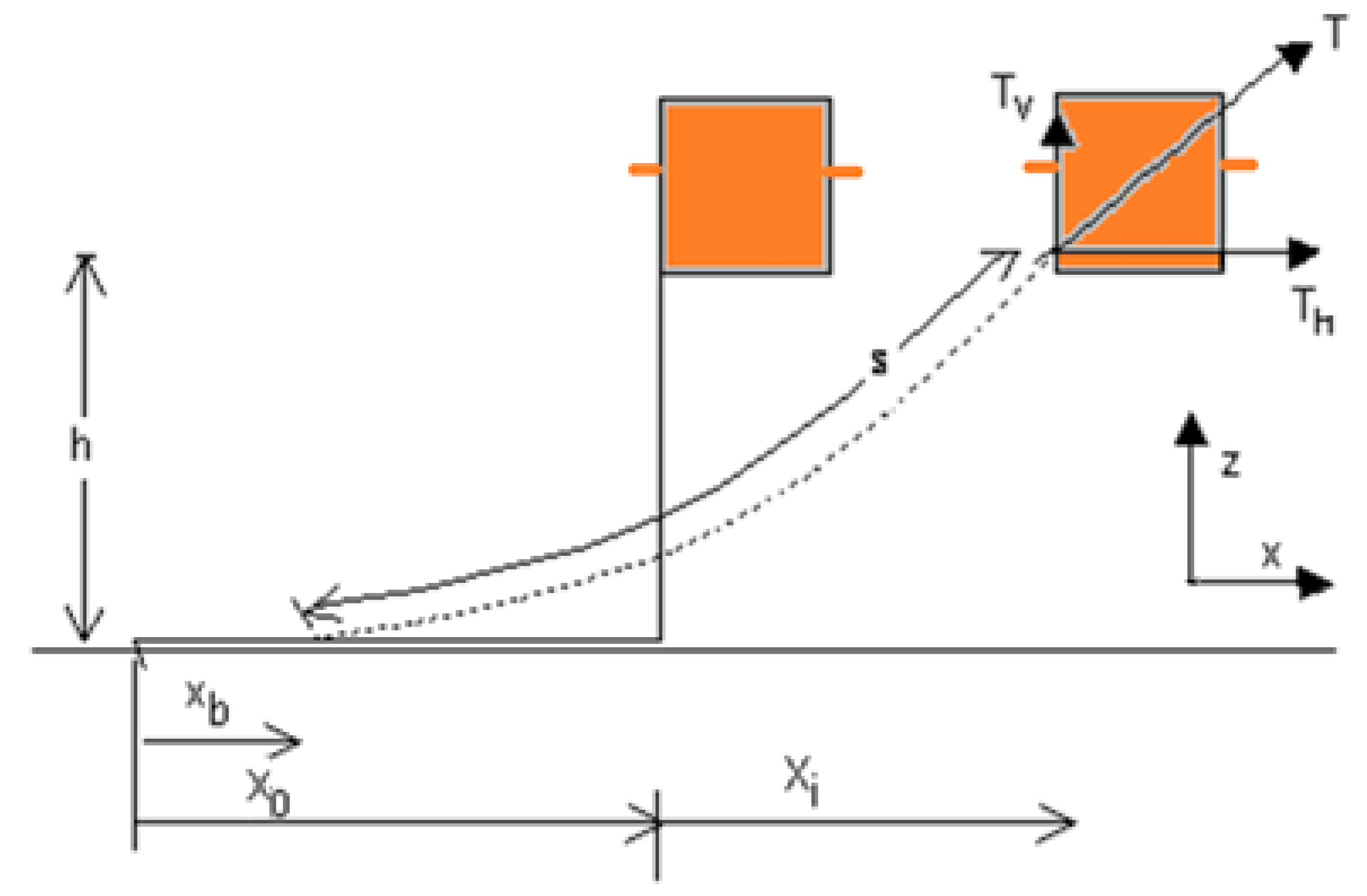
Validation by comparing the hose values for maximum tension.
Table 12.
Validation by comparing the hose values for maximum tension.
| Model | Th, Horizontal Tension (KN) | Tv,Vertical Tension (KN) |
|---|
| Theoretical Model (TM) | 109.30 | 81.60 |
| Finite Element Model (FEM) | 115.40 | 78.50 |
| Model Average = TM/FEM | 0.947 | 1.039 |
Table 13.
Details for Buoy Hydrostatic properties.
Table 13.
Details for Buoy Hydrostatic properties.
| Particulars | Value | Unit |
|---|
| Area | 438.49 | m2 |
| Volume | 344.98 | m3 |
| Buoyancy Force | 1,967,500 | N |
| Centre of Gravity | −2.2 | m |
| Moment of Inertia, Ixx | 4331379.37 | Kg.m2 |
| Moment of Inertia, Iyy | 4486674.11 | Kg.m2 |
| Moment of Inertia, Izz | 4331379.37 | Kg.m2 |
Table 14.
Cases for Sensitivity of zero-crossing period, Tz.
Table 14.
Cases for Sensitivity of zero-crossing period, Tz.
| Cases | HS (m) | TZ (secs) | TP (secs) |
|---|
| TZ Case 1 | 1.87 | 4.10 | 5.27 |
| TZ Case 2 | 1.87 | 6.50 | 8.36 |
| TZ Case 3 | 1.87 | 8.30 | 10.68 |
| TZ Case 4 | 1.87 | 9.66 | 12.43 |
Table 15.
Segment Cases for Hose Segment Lengths.
Table 15.
Segment Cases for Hose Segment Lengths.
| Segment Cases | Section Length (m) | Segment Length (m) | Number of Segments | Segment Clearance |
|---|
| Segment Case 1 | 3.236 | 0.20 | 16 | 0.036 |
| Segment Case 2 | 3.236 | 0.30 | 11 | −0.064 |
| Segment Case 3 | 3.236 | 0.50 | 6 | 0.236 |


