
General and Local Characteristics of Current Marine Heatwave in the Red Sea

 , , ,
, , , 
Abstract
:1. Introduction
2. Data and Methods
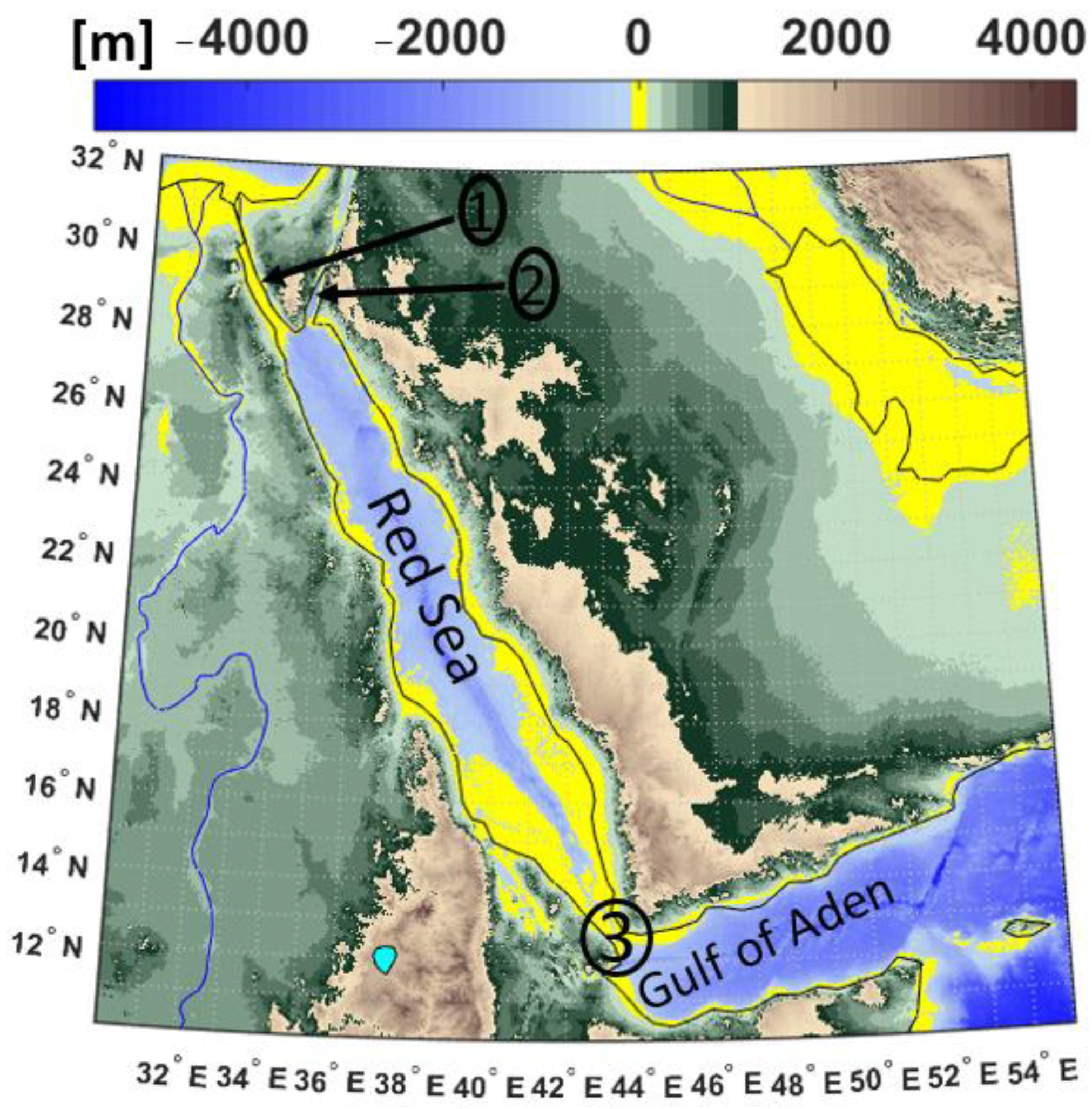
2.1. Data Used
2.2. Extreme Red+ Sea Surface Temperature
2.3. Analyses of the Marine Heat Waves over the Red+
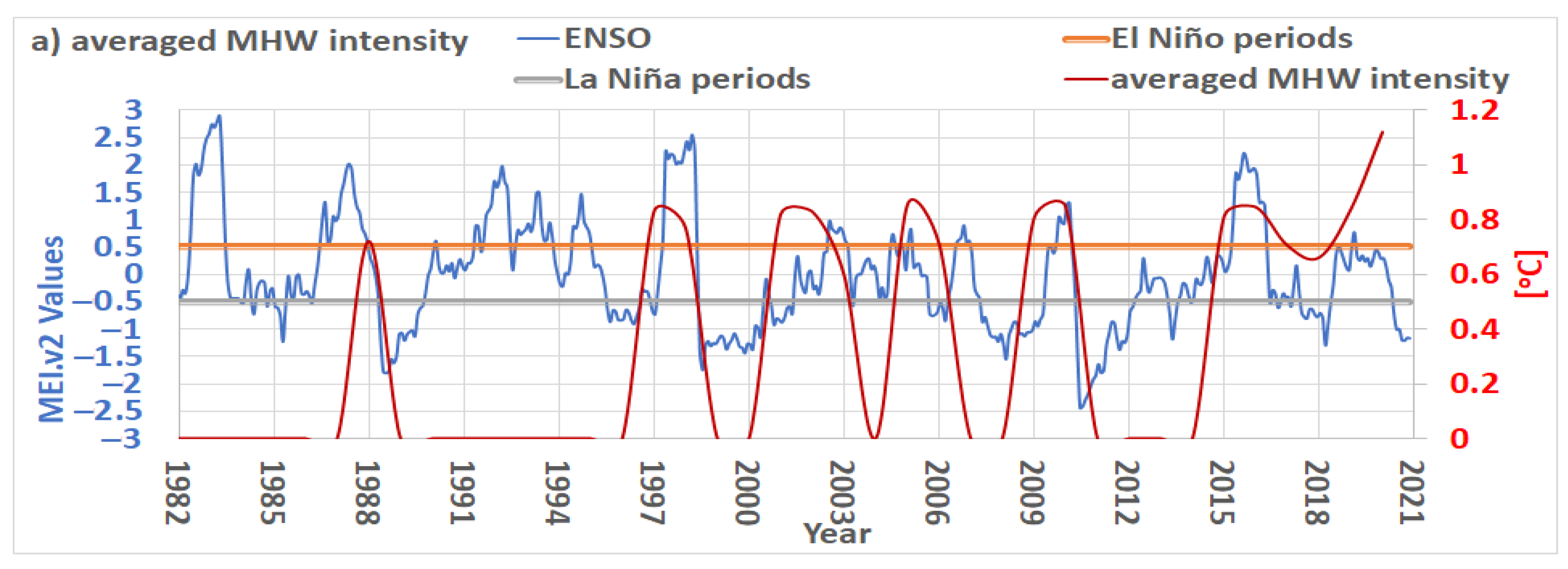
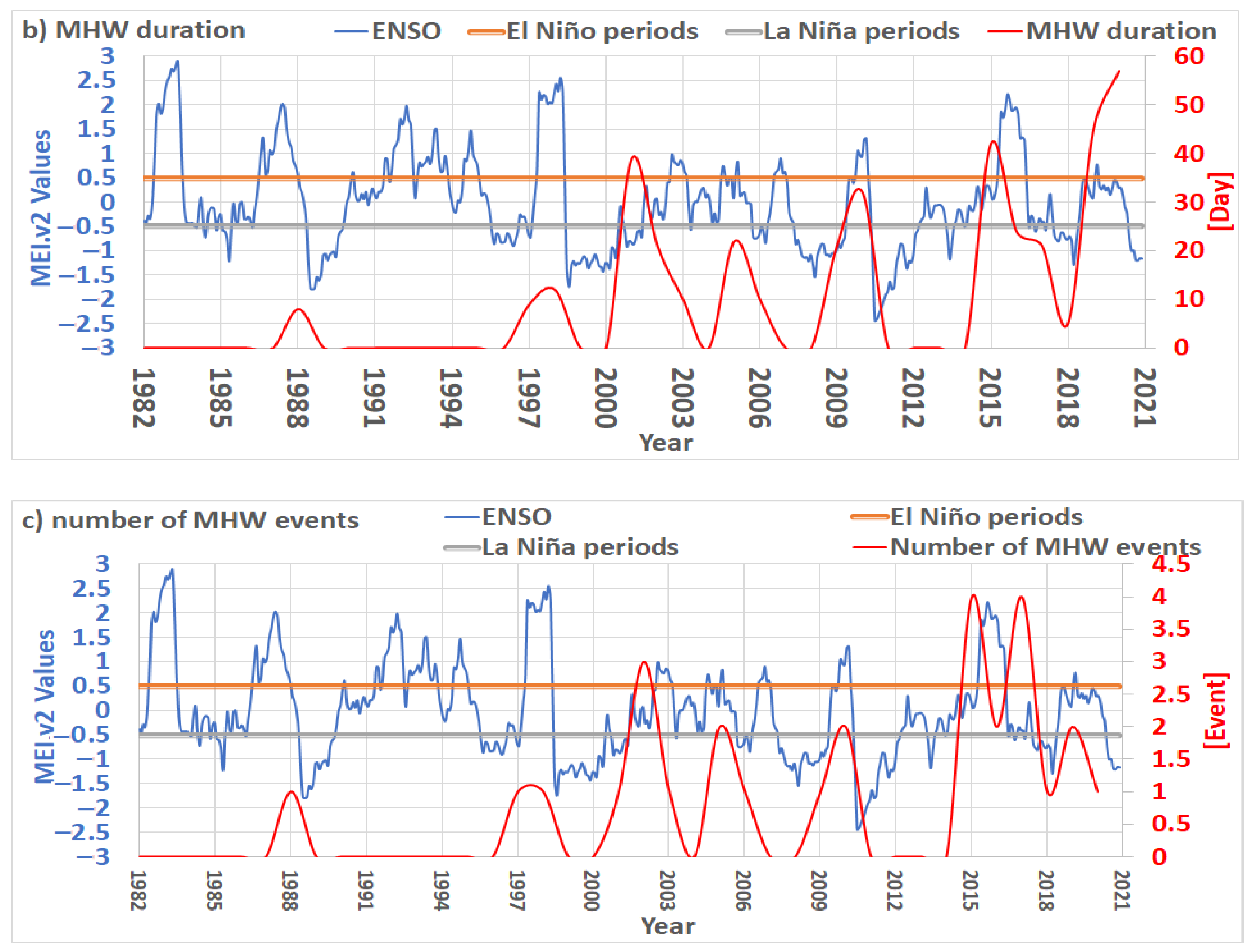
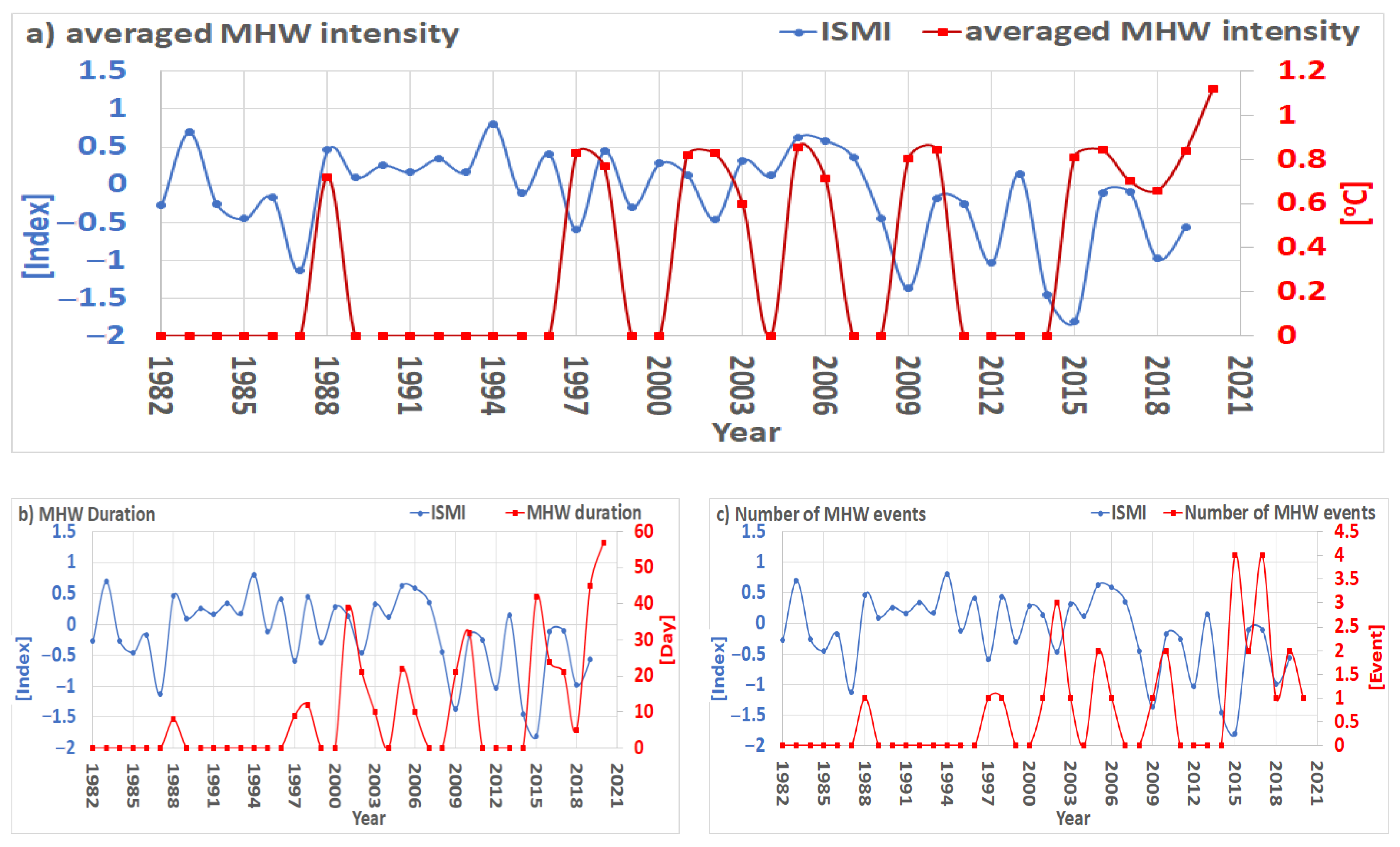
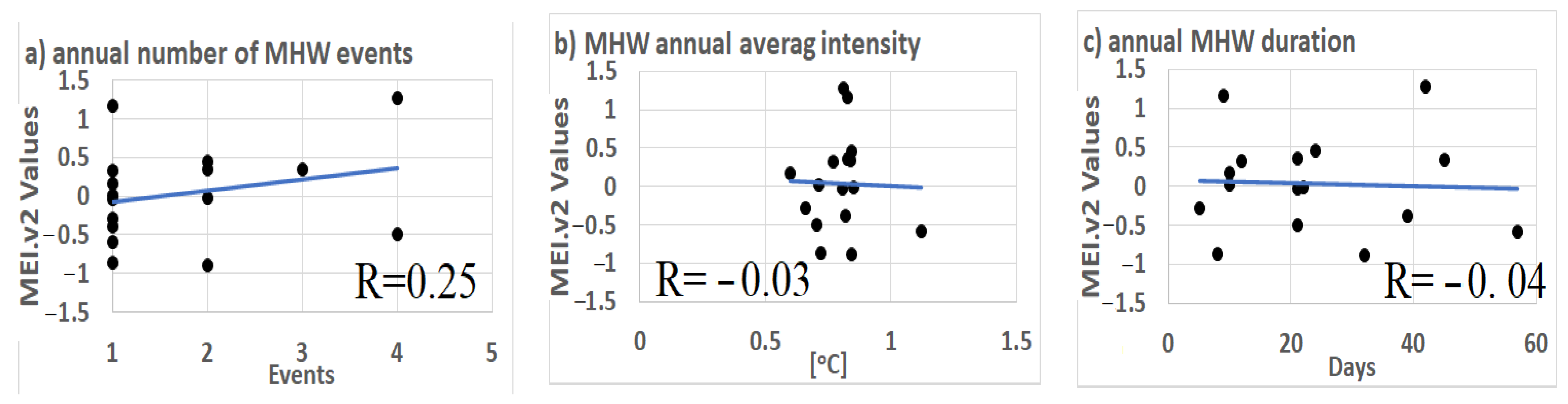
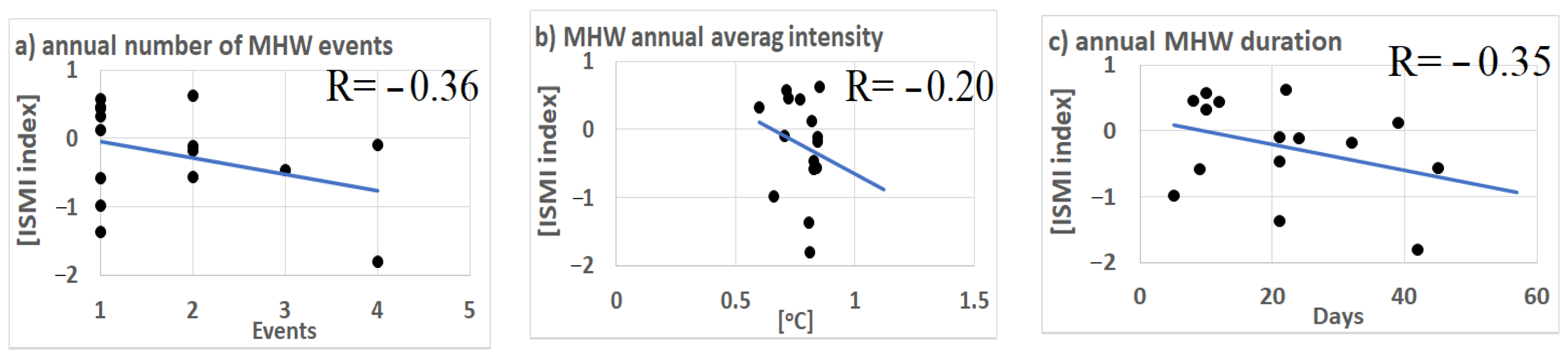
2.3.1. The Role of Climate Variability
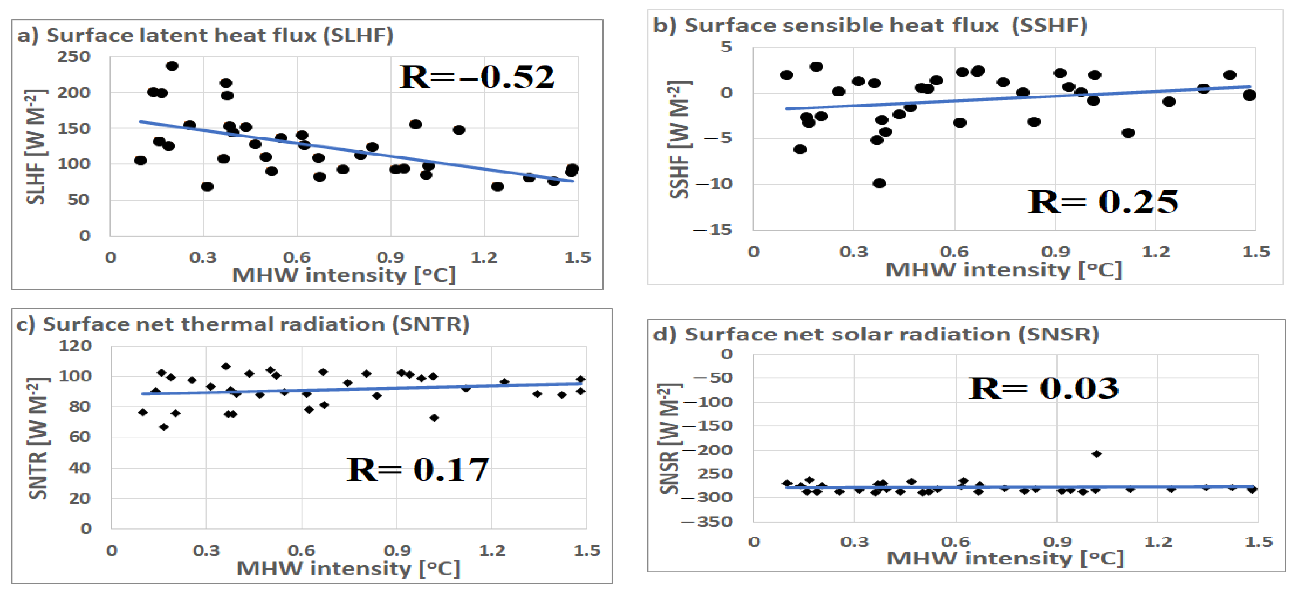
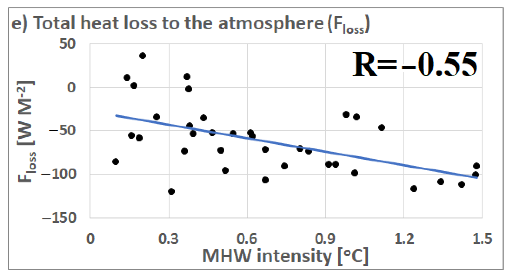
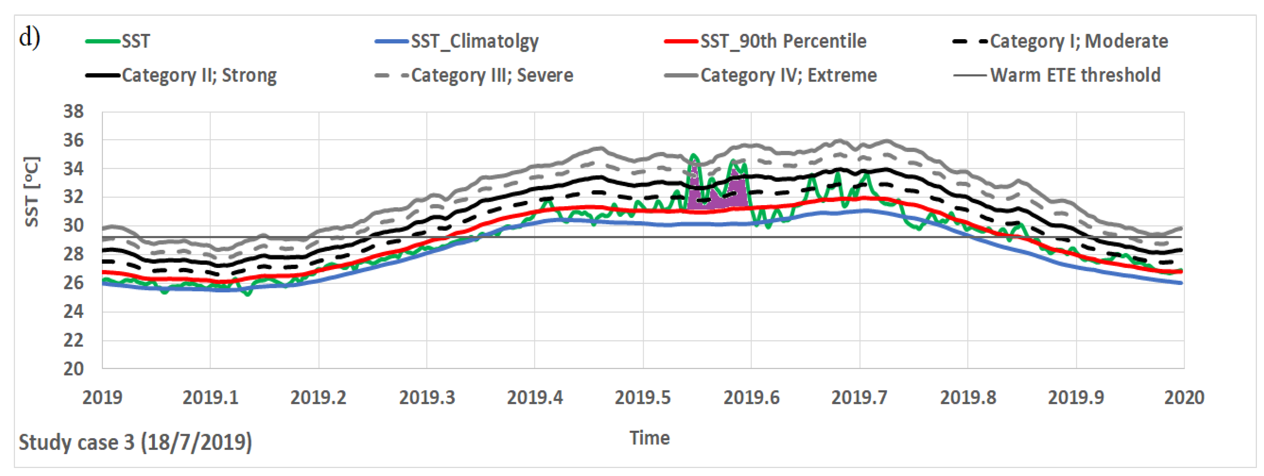
2.3.2. The Role of the Sea Surface Radiation Budget Components
2.4. Main Spatiotemporal Characteristics of MHWs over the Red+
3. Results
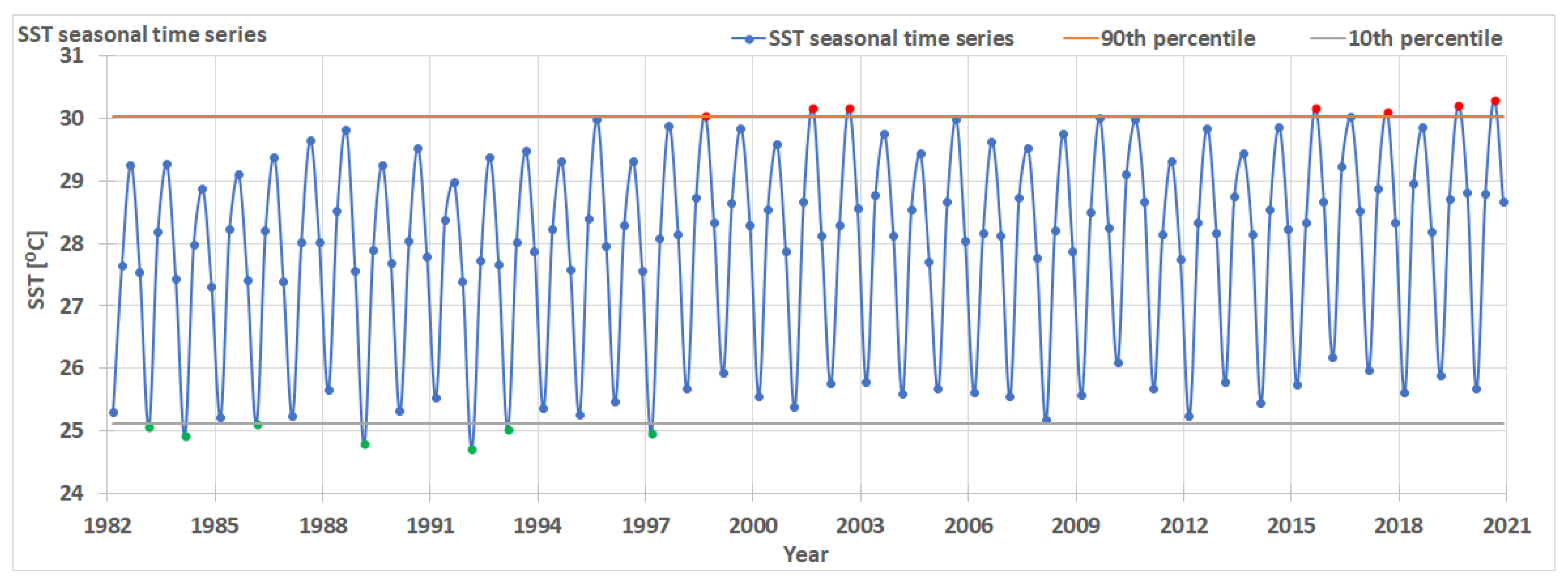
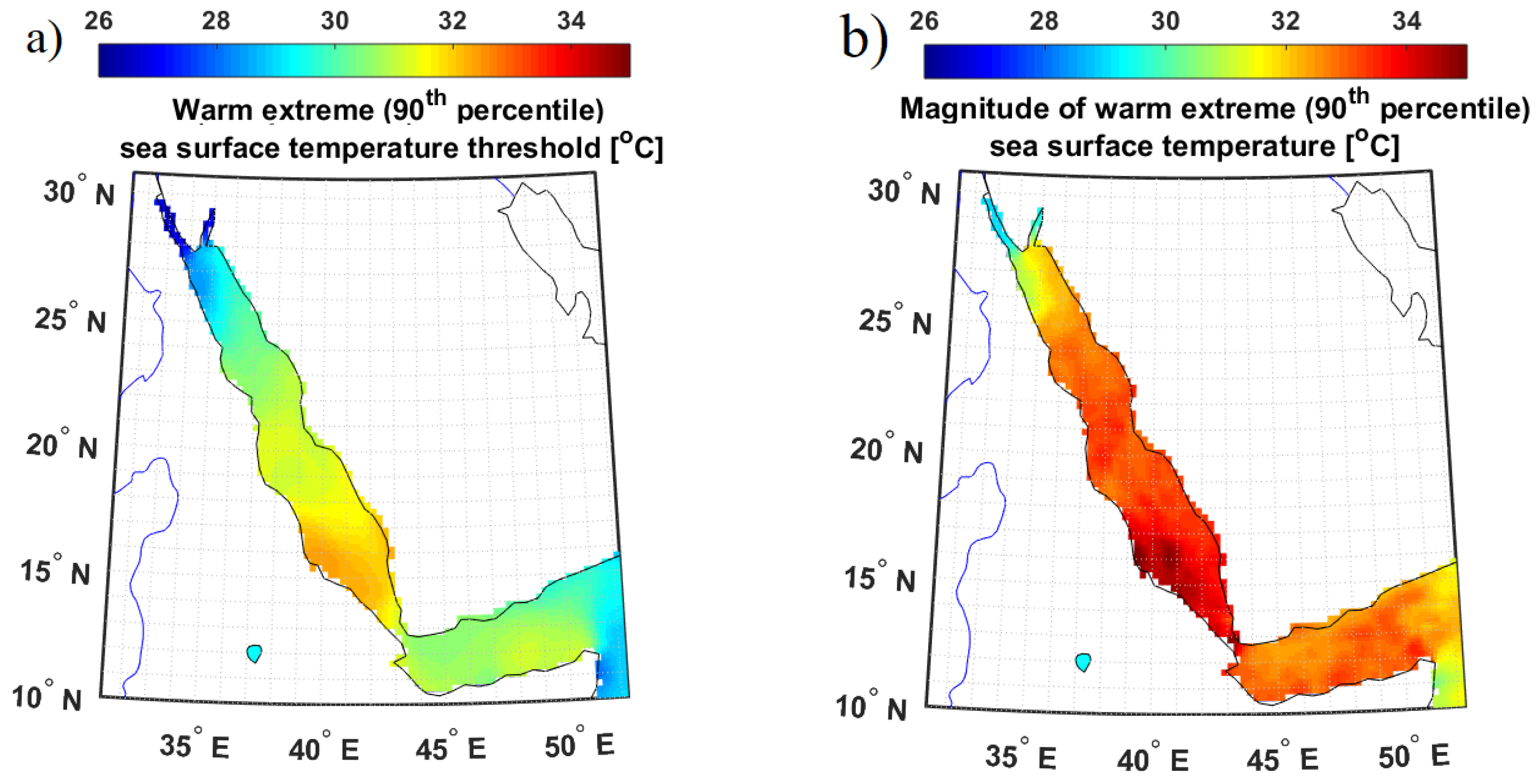
3.1. Extreme Red+ Sea Surface Temperature
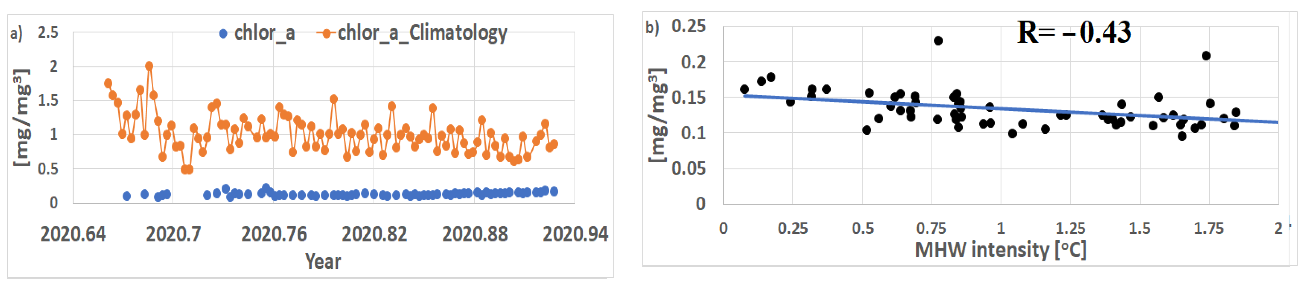
3.2. Marine Heat Waves over the Red+
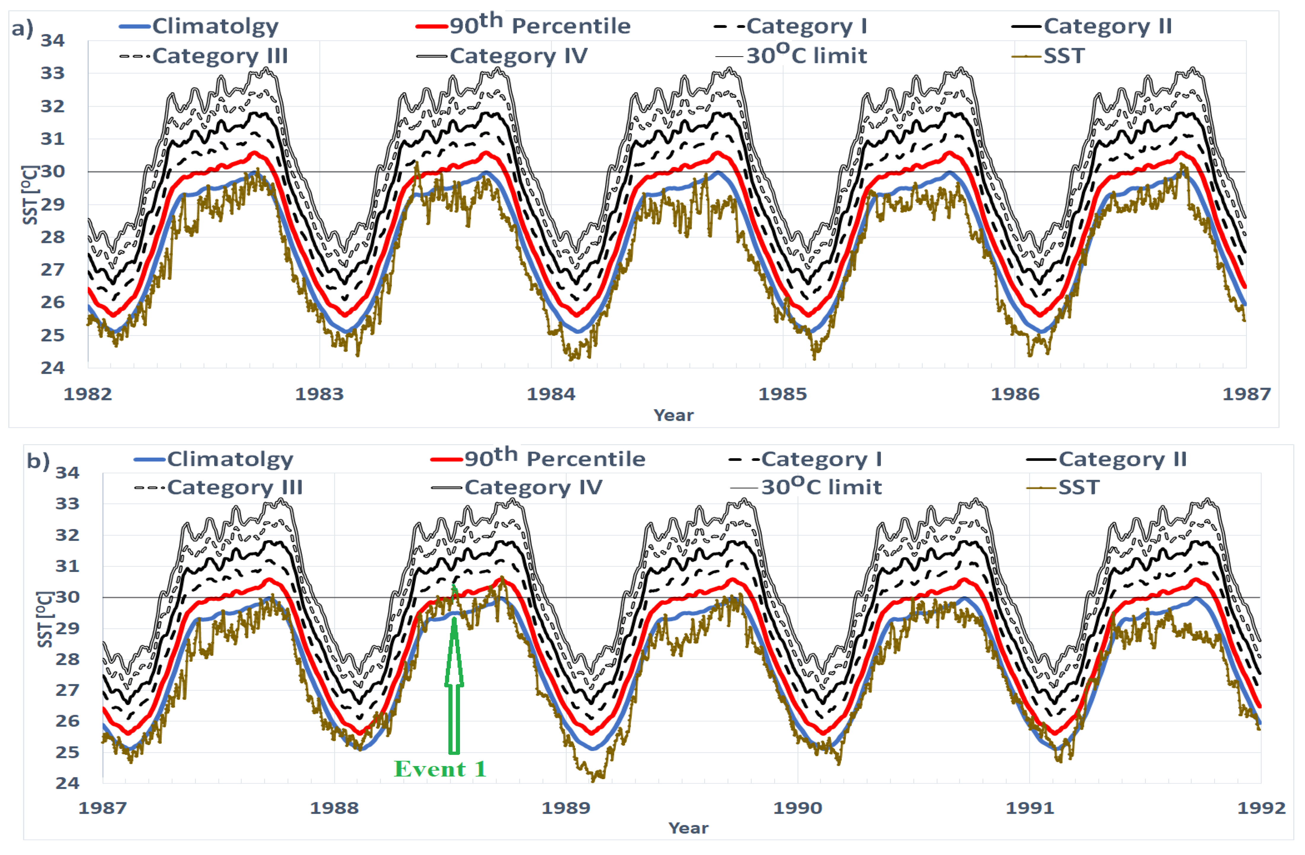
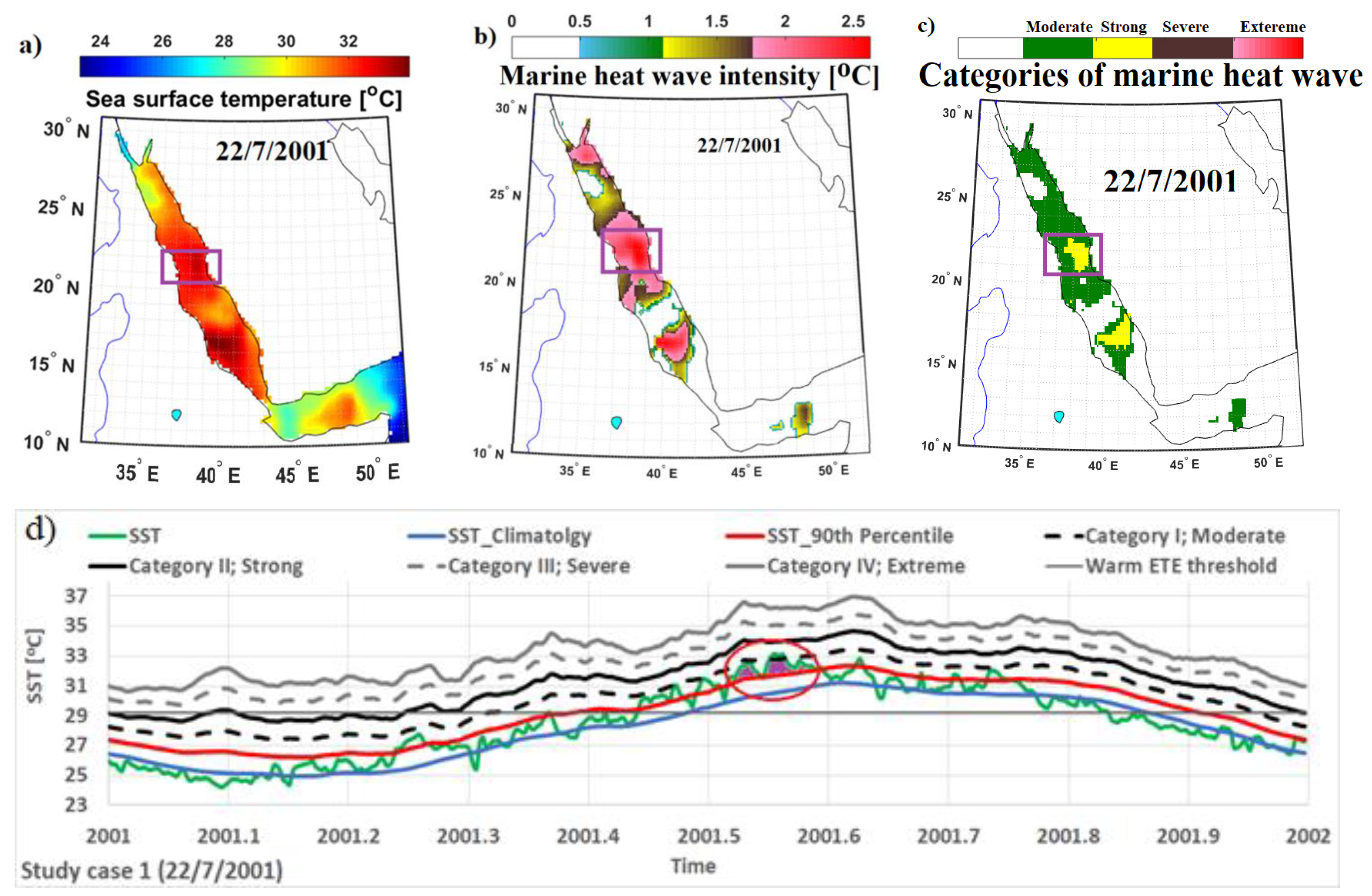
3.3. Selected Study Cases of Marine Heat Waves over the Red+
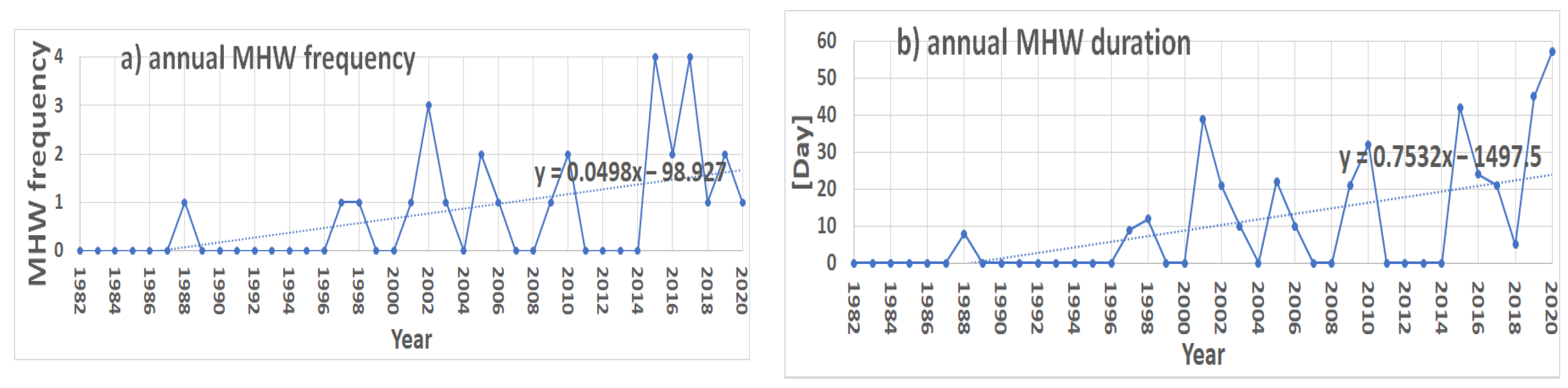
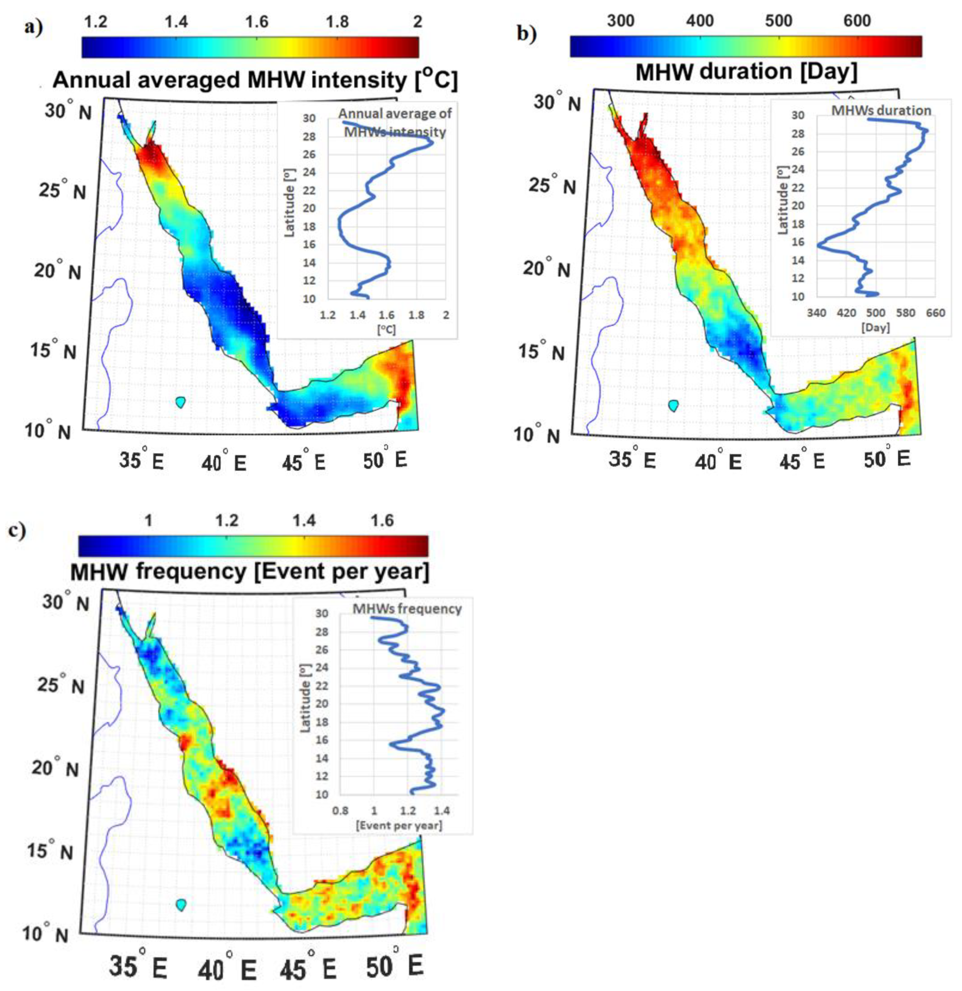
3.4. Main Spatiotemporal Characteristics of Marine MHWs over the Red+
4. Summary Discussion
Author Contributions
Funding
Institutional Review Board Statement
Informed Consent Statement
Data Availability Statement
Acknowledgments
Conflicts of Interest
References
- Hobday, A.J.; Alexander, L.V.; Perkins-Kirkpatrick, S.; Smale, D.; Straub, S.; Oliver, E.; Benthuysen, J.; Burrows, M.; Donat, M.; Feng, M.; et al. A hierarchical approach to defining marine heatwaves. Prog. Oceanogr. 2016, 141, 227–238. [Google Scholar] [CrossRef] [Green Version]
- Sparnocchia, S.; Schiano, M.E.; Picco, P.; Bozzano, R.; Cappelletti, A. The anomalous warming of summer 2003 in the surface layer of the Central Ligurian Sea (Western Mediterranean). Ann. Geophys. 2006, 24, 443–452. [Google Scholar] [CrossRef]
- Oliver, E.C.J.; Benthuysen, J.; Bindoff, N.; Hobday, A.J.; Holbrook, N.J.; Mundy, C.; Perkins-Kirkpatrick, S. The unprecedented 2015/16 Tasman Sea marine heatwave. Nat. Commun. 2017, 8, 16101. [Google Scholar] [CrossRef] [Green Version]
- Holbrook, N.J.; Scannell, H.A.; Gupta, A.S.; Benthuysen, J.A.; Feng, M.; Oliver, E.C.J.; Alexander, L.V.; Burrows, M.T.; Donat, M.G.; Hobday, A.J.; et al. A global assessment of marine heatwaves and their drivers. Nat. Commun. 2019, 10, 1–13. [Google Scholar] [CrossRef]
- Chaidez, V.; Dreano, D.; Agusti, S.; Duarte, C.M.; Hoteit, I. Decadal trends in Red Sea maximum surface temperature. Sci. Rep. 2017, 7, 8144. [Google Scholar] [CrossRef] [Green Version]
- Shaltout, M. Recent sea surface temperature trends and future scenarios for the Red Sea. Oceanologia 2019, 61, 484–504. [Google Scholar] [CrossRef]
- Olita, A.; Sorgente, R.; Ribotti, A.; Natale, S.; Gaberšek, S. Effects of the 2003 European heatwave on the Central Mediterranean Sea surface layer: A numerical simulation. Ocean Sci. Discuss. 2006, 3, 85–125. [Google Scholar]
- Ibrahim, O.; Mohamed, B.; Nagy, H. Spatial Variability and Trends of Marine Heat Waves in the Eastern Mediterranean Sea over 39 Years. J. Mar. Sci. Eng. 2021, 9, 643. [Google Scholar] [CrossRef]
- Pearce, A.F.; Feng, M. The rise and fall of the ‘marine heat wave’ off Western Australia during the summer of 2010/11. J. Mar. Syst. 2013, 112, 139–156. [Google Scholar] [CrossRef]
- Benthuysen, J.A.; Oliver EC, J.; Feng, M.; Marshall, A.G. Extreme marine warming across tropical Australia during austral summer 2015–16. J. Geophys. Res. 2018, 123, 1301–1326. [Google Scholar] [CrossRef]
- Bond, N.A.; Cronin, M.F.; Freeland, H.; Mantua, N. Causes and impacts of the 2014 warm anomaly in the NE Pacific. Geophys. Res. Lett. 2015, 42, 3414–3420. [Google Scholar] [CrossRef]
- Chen, K.; Gawarkiewicz, G.G.; Lentz, S.J.; Bane, J.M. Diagnosing the warming of the Northeastern US Coastal Ocean in 2012: A linkage between the atmospheric jet stream variability and ocean response. J. Geophys. Res. Ocean. 2014, 119, 218–227. [Google Scholar] [CrossRef] [Green Version]
- Hughes, T.P.; Kerry, J.T.; Álvarez-Noriega, M.; Álvarez-Romero, J.; Anderson, K.; Baird, A.H.; Babcock, R.; Beger, M.; Bellwood, D.R.; Berkelmans, R.; et al. Global warming and recurrent mass bleaching of corals. Nature 2017, 543, 373–377. [Google Scholar] [CrossRef] [PubMed]
- Caputi, N.; Kangas, M.; Denham, A.; Feng, M.; Pearce, A.; Hetzel, Y.; Chandrapavan, A. Management adaptation of invertebrate fisheries to an extreme marine heat wave event at a global warming hot spot. Ecol. Evol. 2016, 6, 3583–3593. [Google Scholar] [CrossRef]
- Garrabou, J.; Coma, R.; Bensoussan, N.; Bally, M.; Chevaldonné, P.; Ciglianos, M.; Díaz, D.; Harmelin, J.G.; Gambi, M.C.; Kersting, D.K.; et al. Mass mortality in Northwestern Mediterranean rocky benthic communities: Effects of the 2003 heat wave. Glob. Chang. Biol. 2009, 15, 1090–1103. [Google Scholar] [CrossRef]
- Mills, K.E.; Pershing, A.J.; Brown, C.J.; Chen, Y.; Chiang, F.-S.; Holland, D.; Lehuta, S.; Nye, J.; Sun, J.C.; Thomas, A.C.; et al. Fisheries Management in a Changing Climate: Lessons From the 2012 Ocean Heat Wave in the Northwest Atlantic. Oceanography 2013, 26. [Google Scholar] [CrossRef] [Green Version]
- Cavole, L.M.; Demko, A.M.; Diner, R.E.; Giddings, A.; Koester, I.; Pagniello, C.M.L.S.; Paulsen, M.-L.; Ramirez-Valdez, A.; Schwenck, S.M.; Yen, N.K. Biological impacts of the 2013–2015 warm-water anomaly in the Northeast Pacific: Winners, losers, and the future. Oceanography 2016, 29, 273–285. [Google Scholar] [CrossRef] [Green Version]
- Bindoff, N.L.; Stott, P.A.; AchutaRao, K.M.; Allen, M.R.; Gillett, N.; Gutzler, D.; Hansingo, K.; Hegerl, G.; Hu, Y.; Jain, S.; et al. Detection and attribution of climate change: From global to regional. In Climate Change 2013: The Physical Science Basis; Contribution of Working Group 1 to the Fifth Assessment Report of the Intergovernmental Panel on Climate Change; Stocker, B.D., Qin, D., Plattner, G.-K., Tignor, M.M.B., Allen, S.K., Boschung, J., Nauels, A., Xia, Y., Bex, V., Midgley, P.M., Eds.; Cambridge University Press: Cambridge, UK, 2013; pp. 867–952. [Google Scholar]
- Hodgkinson, J.H.; Hobday, A.J.; Pinkard, E.A. Climate adaptation in Australia’s resource-extraction industries: Ready or not? Reg. Environ. Chang. 2014, 14, 1663–1678. [Google Scholar] [CrossRef]
- Genevier, L.G.C.; Jamil, T.; Raitsos, D.E.; Krokos, G.; Hoteit, I. Marine heatwaves reveal coral reef zones susceptible to bleaching in the Red Sea. Glob. Chang. Biol. 2019, 25, 2338–2351. [Google Scholar] [CrossRef] [Green Version]
- Darmaraki, S.; Somot, S.; Sevault, F.; Nabat, P.; Narvaez, W.D.C.; Cavicchia, L.; Djurdjevic, V.; Li, L.; Sannino, G.; Sein, D.V. Future evolution of Marine Heatwaves in the Mediterranean Sea. Clim. Dyn. 2019, 53, 1371–1392. [Google Scholar] [CrossRef] [Green Version]
- Reynolds, R.W.; Smith, T.M.; Liu, C.; Chelton, D.B.; Casey, K.; Schlax, M.G. Daily High-Resolution-Blended Analyses for Sea Surface Temperature. J. Clim. 2007, 20, 5473–5496. [Google Scholar] [CrossRef]
- Reynolds, R.W. What’s New in Version 2 of Daily Optimum Interpolation (OI) Sea Surface Temperature (SST) Analysis. 2009. 10p. Available online: https://www.ncdc.noaa.gov/sites/default/files/attachments/Reynolds2009_oisst_daily_v02r00_version2-features.pdf (accessed on 19 August 2021).
- Banzon, V.; Reynolds, R.; National Center for Atmospheric Research Staff (Eds.) The Climate Data Guide: SST Data: NOAA Optimal Interpolation (OI) SST Analysis, Version 2 (OISSTv2) 1x1. 2018. Available online: https://climatedataguide.ucar.edu/climate-data/sst-data-noaa-optimal-interpolation-oi-sst-analysis-version-2-oisstv2-1x1 (accessed on 17 December 2018).
- Worley, S.J.; Woodruff, S.D.; Reynolds, R.W.; Lubker, S.J.; Lott, N. ICOADS release 2.1 data and products. Int. J. Climatol. 2005, 25, 823–842. [Google Scholar] [CrossRef]
- Karnauskas, K.B.; Jones, B.H. The Interannual Variability of Sea Surface Temperature in the Red Sea from 35 Years of Satellite and In Situ Observations. J. Geophys. Res. Oceans 2018, 123, 5824–5841. [Google Scholar] [CrossRef]
- SeaWiFS Mission Page. NASA Ocean Biology Processing Group, Greenbelt, MD, USA. Maintained by NASA Ocean Biology Distibuted Active Archive Center (OB.DAAC), Goddard Space Flight Center, Greenbelt MD. 2019. Available online: https://oceancolor.gsfc.nasa.gov/data/10.5067/ORBVIEW-2/SEAWIFS/L2/OC/2018/ (accessed on 16 August 2021).
- Brewin, R.J.; Raitsos, D.E.; Pradhan, Y.; Hoteit, I. Comparison of chlorophyll in the Red Sea derived from MODIS-Aqua and in vivo fluorescence. Remote. Sens. Environ. 2013, 136, 218–224. [Google Scholar] [CrossRef]
- Eladawy, A.; Nadaoka, K.; Negm, A.; Abdel-Fattah, S.; Hanafy, M.; Shaltout, M. Characterization of the northern Red Sea’s oceanic features with remote sensing data and outputs from a global circulation model. Oceanologia 2017, 59, 213–237. [Google Scholar] [CrossRef]
- Zhang, T.; Hoell, A.; Perlwitz, J.; Eischeid, J.; Murray, D.; Hoerling, M.; Hamill, T.M. Towards Probabilistic Multivariate ENSO Monitoring. Geophys. Res. Lett. 2019, 46, 10532–10540. [Google Scholar] [CrossRef]
- Wang, B.; Wu, R.; Lau, K. Interannual variability of Asian summer monsoon: Contrast between the Indian and western North Pacific-East Asian monsoons. J. Climatol. 2001, 14, 4073–4090. [Google Scholar] [CrossRef]
- Hersbach, H.; Bell, B.; Berrisford, P.; Hirahara, S.; Horanyi, A.; Muñoz-Sabater, J.; Nicolas, J.; Peubey, C.; Radu, R.; Schepers, D.; et al. The ERA5 global reanalysis. Q. J. R. Meteorol. Soc. 2020, 146, 1999–2049. [Google Scholar] [CrossRef]
- Copernicus Climate Change Service (C3S). ERA5: Fifth Generation of ECMWF Atmospheric Reanalyses of the Global Climate. Copernicus Climate Change Service Climate Data Store (CDS). 2017. Available online: https://cds.climate.copernicus.eu/cdsapp#!/home (accessed on 29 January 2020).
- Hobday, A.; Oliver, E.C.J.; Gupta, A.S.; Benthuysen, J.A.; Burrows, M.T.; Donat, M.G.; Holbrook, N.J.; Moore, P.J.; Thomsen, M.S.; Wernberg, T.; et al. Categorizing and naming marine heatwaves. Oceanography 2018, 31, 162–173. [Google Scholar]
- Oliver, E.C.J.; Donat, M.G.; Burrows, M.; Moore, P.; Smale, D.A.; Alexander, L.V.; Benthuysen, J.; Feng, M.; Gupta, A.S.; Hobday, A.J.; et al. Longer and more frequent marine heatwaves over the past century. Nat. Commun. 2018, 9, 1324. [Google Scholar] [CrossRef]


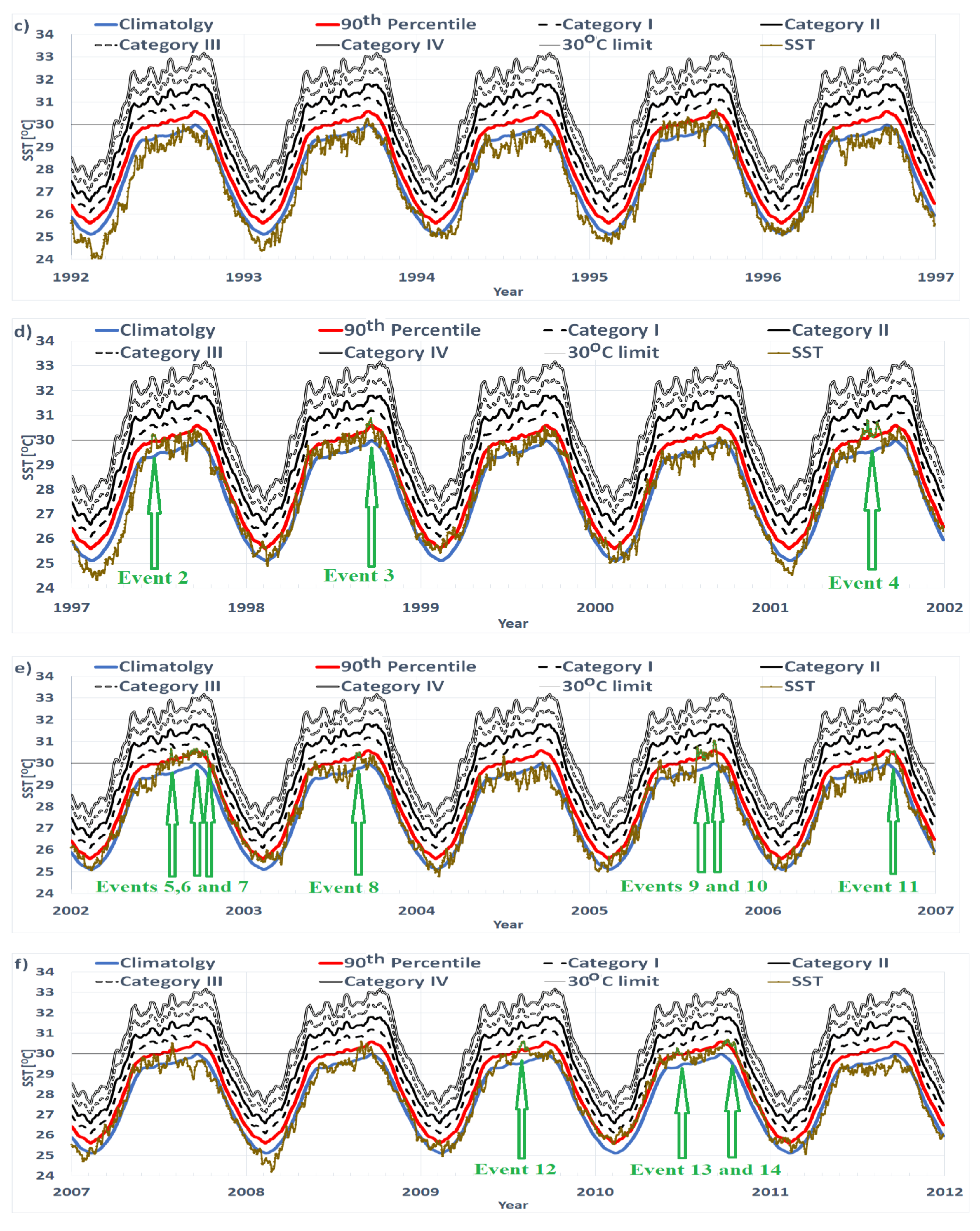
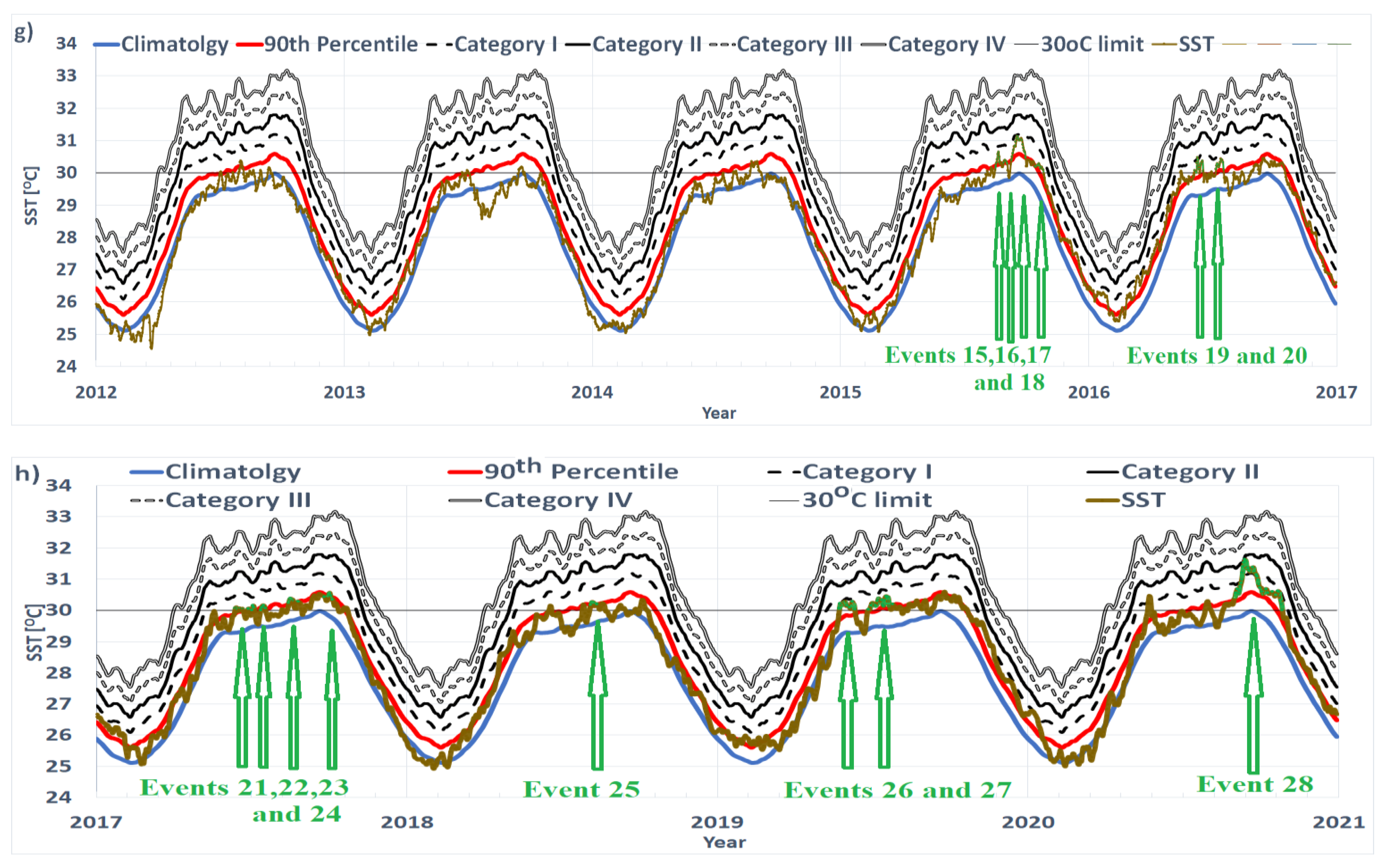
| Event Number. | Date of Peak Intensity | The Total Duration of the Event | Category | Intensity (Calculated above the Climatological Mean) | P (%) | |||||||
|---|---|---|---|---|---|---|---|---|---|---|---|---|
| First Day | Last Day | Total Days without Gaps | Imax (°C) | Imean (°C) | Icun (°C-day) | Moderate (M) | Strong (Sg) | Severe (Sv) | Extreme (E) | |||
| 1 | 8 July 1988 | 6 July 1988 | 13 July 1988 | 8 | M | 0.88 | 0.72 | 5.76 | 100 | - | - | - |
| 2 | 20 June 1997 | 18 June 1997 | 26 June 1997 | 9 | M | 0.90 | 0.82 | 7.45 | 100 | - | - | - |
| 3 | 19 September 1998 | 9 September 1998 | 20 September 1998 | 12 | M | 0.91 | 0.77 | 9.21 | 100 | - | - | - |
| 4 | 22 July 2001 | 10 July 2001 | 22 August 2001 | 39 | M | 1.30 | 0.82 | 36.03 | 89 | - | - | - |
| 5 | 31 July 2002 | 29 July 2002 | 2 August 2002 | 5 | M | 1.13 | 0.91 | 4.58 | 100 | - | - | - |
| 6 | 11 August 2002 | 9 August 2002 | 14 August 2002 | 6 | M | 0.74 | 0.68 | 4.1 | 100 | - | - | - |
| 7 | 15 October 2002 | 5 October 2002 | 16 October 2002 | 10 | M | 1.04 | 0.85 | 4.26 | 85 | - | - | - |
| 8 | 27 August 2003 | 26 August 2003 | 4 September 2003 | 10 | M | 0.73 | 0.60 | 5.14 | 100 | - | - | - |
| 9 | 16 August 2005 | 15 August 2005 | 31 September 2005 | 15 | M | 1.11 | 0.79 | 11.93 | 89 | - | - | - |
| 10 | 22 September 2005 | 19 September 2005 | 25 September 2005 | 7 | M | 1.04 | 0.91 | 6.37 | 100 | - | - | - |
| 11 | 7 October 2006 | 29 September 2006 | 8 October 2006 | 10 | M | 0.81 | 0.70 | 7.08 | 100 | - | - | - |
| 12 | 5 August 2009 | 23 July 2009 | 13 Aug2009 | 21 | M | 1.05 | 0.81 | 17.7 | 96 | - | - | - |
| 13 | 21 June 2010 | 18 June 2010 | 24 June 2010 | 7 | M | 0.93 | 0.82 | 5.74 | 100 | - | - | - |
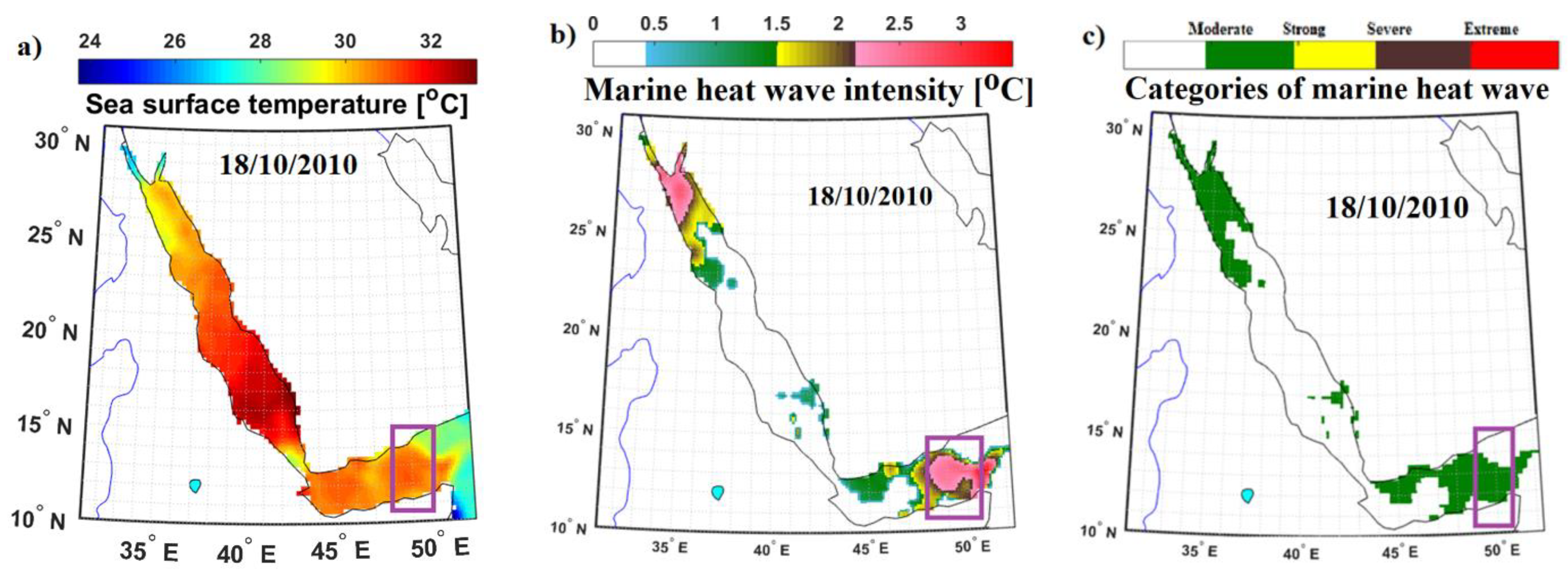
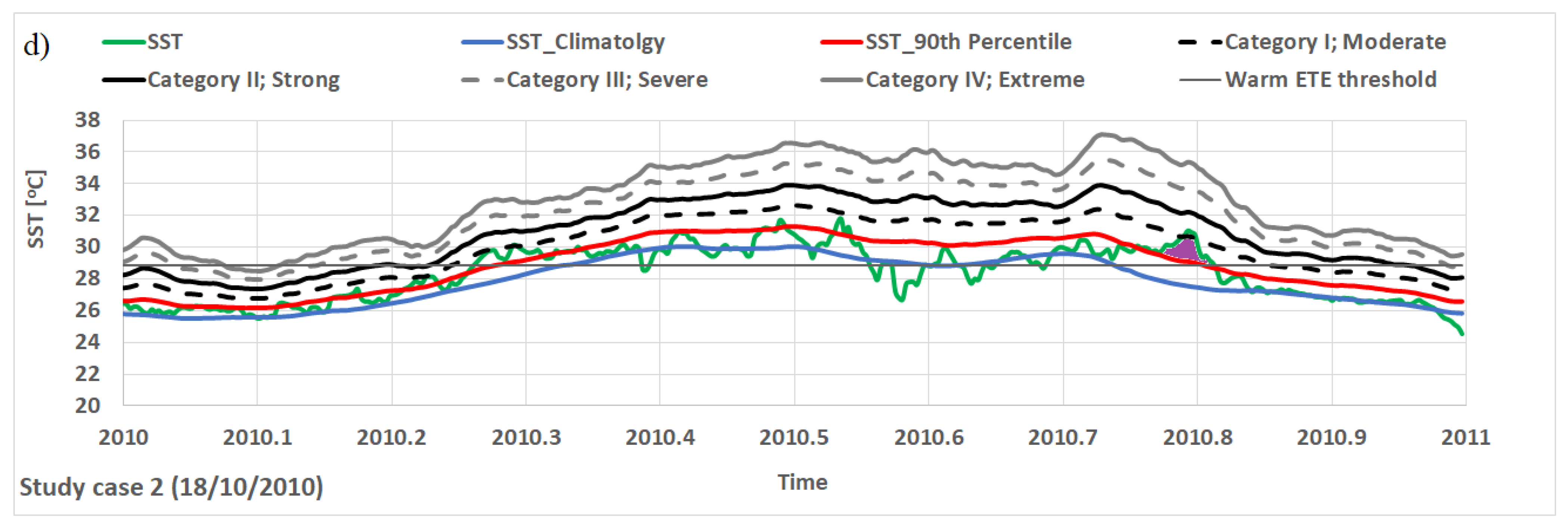
| 14 | 18 October 2010 | 29 September 2010 | 23 October 2010 | 25 | M | 1.15 | 0.87 | 21.6 | 100 | - | - | - |
| 15 | 21 August 2015 | 18 August 2015 | 23 August 2015 | 6 | M | 0.96 | 0.78 | 4.66 | 100 | - | - | - |
| 16 | 31 August 2015 | 29 August 2015 | 2 September 2015 | 5 | M | 0.61 | 0.54 | 2.68 | 100 | - | - | - |
| 17 | 18 September 2015 | 9 September 2015 | 29 September 2015 | 21 | M | 1.18 | 0.94 | 19.77 | 100 | - | - | - |
| 18 | 24 October 2015 | 17 October 2015 | 26 October 2015 | 10 | M | 1.04 | 0.94 | 9.38 | 100 | - | - | - |
| 19 | 10 June 2016 | 6 June 2016 | 18 June 2016 | 12 | M | 1.19 | 0.90 | 10.97 | 92 | - | - | - |
| 20 | 14 July 2016 | 7 July 2016 | 18 July 2016 | 12 | M | 0.92 | 0.78 | 9.31 | 100 | - | - | - |
| 21 | 18 June 2017 | 17 June 2017 | 21 June 2017 | 5 | M | 0.75 | 0.72 | 3.60 | 100 | - | - | - |
| 22 | 16 July 2017 | 14 July 2017 | 18 July 2017 | 5 | M | 0.66 | 0.63 | 3.11 | 100 | - | - | - |
| 23 | 17 August 2017 | 15 August 2017 | 20 August 2017 | 6 | M | 0.71 | 0.66 | 3.97 | 100 | - | - | - |
| 24 | 22 October 2017 | 19 October 2017 | 23 October 2017 | 5 | M | 0.86 | 0.80 | 4.01 | 100 | - | - | - |
| 25 | 6 August 2018 | 5 August 2018 | 9 August 2018 | 5 | M | 0.72 | 0.66 | 3.30 | 100 | - | - | - |
| 26 | 25 May 2019 | 24 May 2019 | 11 June 2019 | 19 | M | 1.05 | 0.91 | 17.28 | 100 | - | - | - |
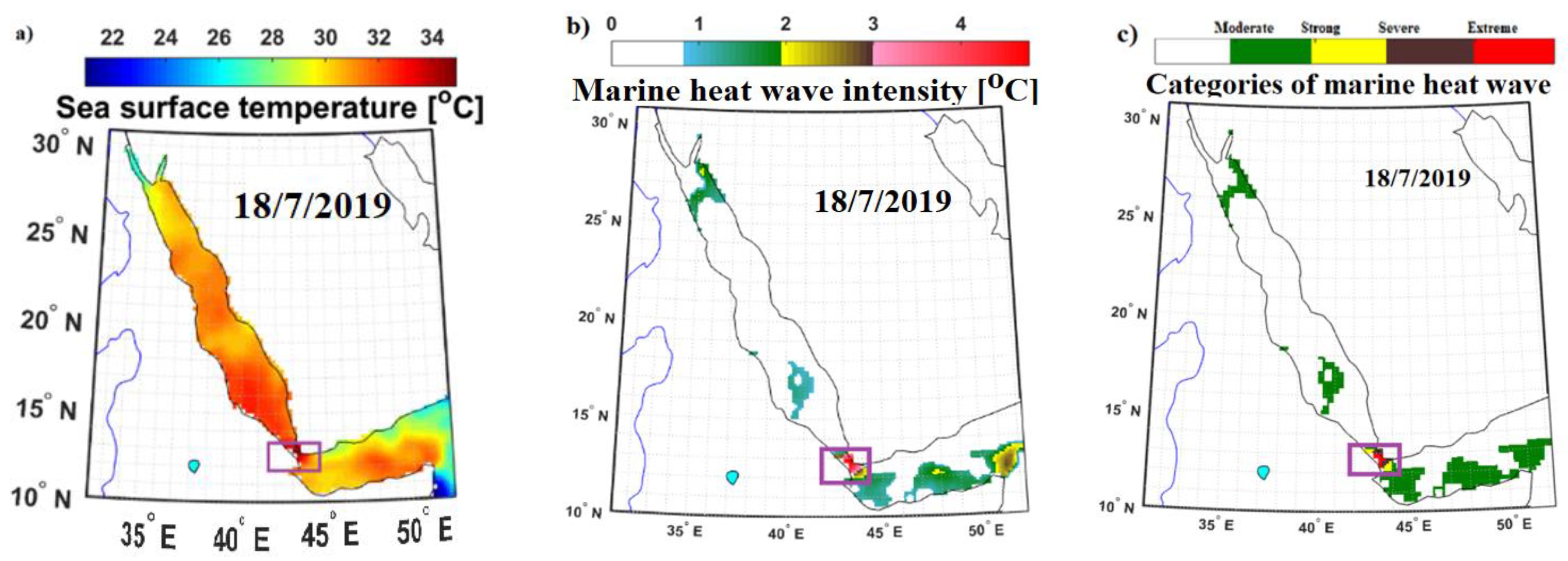
| 27 | 18 July 2019 | 27 June 2019 | 22 July 2019 | 26 | M | 0.97 | 0.77 | 19.90 | 100 | - | - | - |
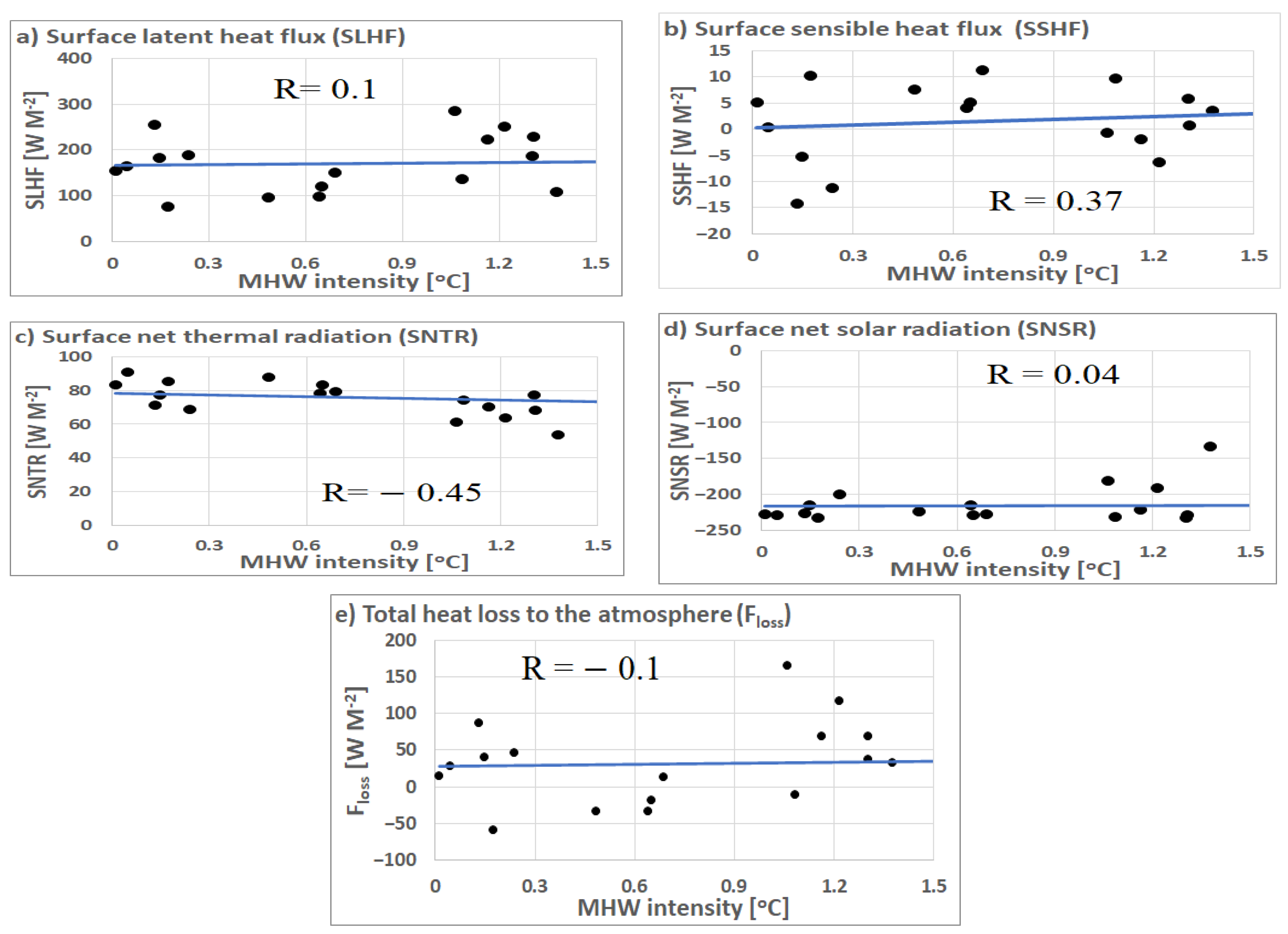
| 28 | 13 September 2020 | 31 August 2020 | 26 October 2020 | 57 | Sg | 1.76 | 1.11 | 63.78 | 69 | 31 | - | - |
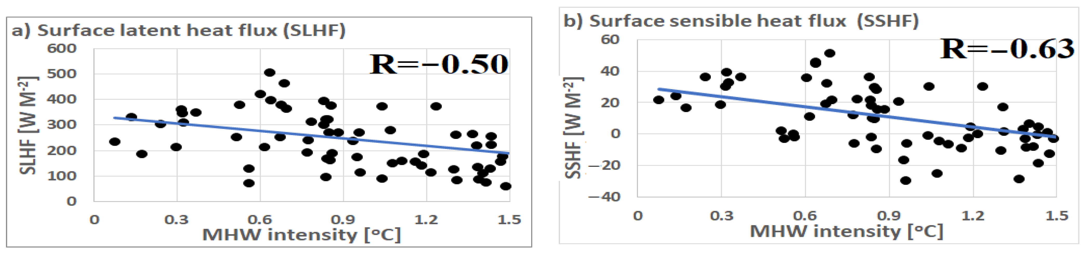
| SLHF | SSHF | SNTR | SNSR | Floss | |
|---|---|---|---|---|---|
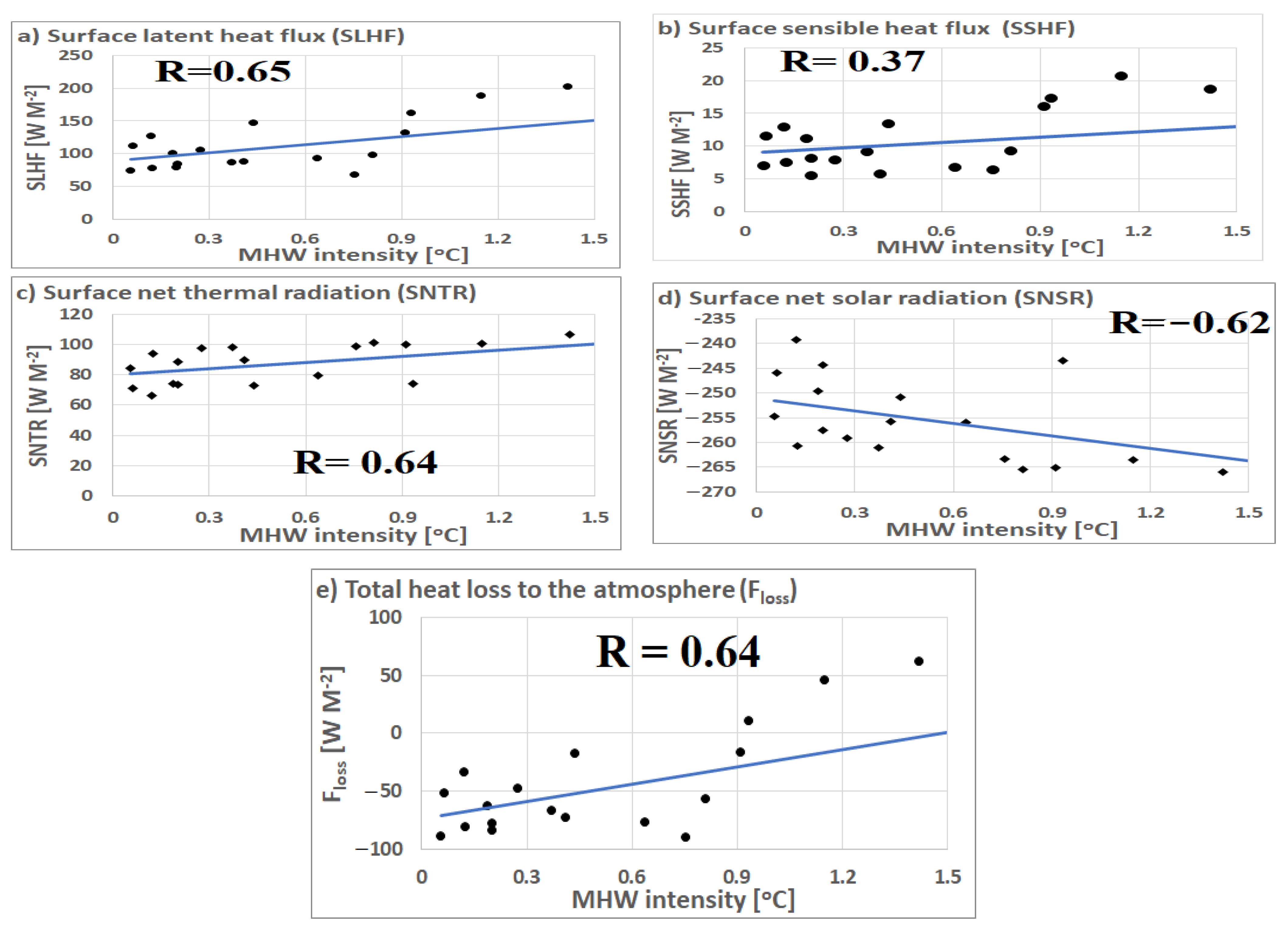
| Range over the study period | 41 to 287 | −14 to 90 | 50 to 163 | −294 to −99 | −152 to 287 |
| Range during the marine heat wave events | 57 to 206 | −10 to 13 | 56 to 101 | −279 to −210 | −133 to −7 |
Publisher’s Note: MDPI stays neutral with regard to jurisdictional claims in published maps and institutional affiliations. |
© 2021 by the authors. Licensee MDPI, Basel, Switzerland. This article is an open access article distributed under the terms and conditions of the Creative Commons Attribution (CC BY) license (https://creativecommons.org/licenses/by/4.0/).
Share and Cite
Bawadekji, A.; Tonbol, K.; Ghazouani, N.; Becheikh, N.; Shaltout, M. General and Local Characteristics of Current Marine Heatwave in the Red Sea. J. Mar. Sci. Eng. 2021, 9, 1048. https://doi.org/10.3390/jmse9101048
Bawadekji A, Tonbol K, Ghazouani N, Becheikh N, Shaltout M. General and Local Characteristics of Current Marine Heatwave in the Red Sea. Journal of Marine Science and Engineering. 2021; 9(10):1048. https://doi.org/10.3390/jmse9101048
Chicago/Turabian StyleBawadekji, Abdulhakim, Kareem Tonbol, Nejib Ghazouani, Nidhal Becheikh, and Mohamed Shaltout. 2021. "General and Local Characteristics of Current Marine Heatwave in the Red Sea" Journal of Marine Science and Engineering 9, no. 10: 1048. https://doi.org/10.3390/jmse9101048