Article

Intercomparison of Assimilated Coastal Wave Data in the Northwestern Pacific Area

Department of Physics and Earth Sciences, University of the Ryukyus, Senbaru 1, Nishihara-cho, Okinawa 903-0213, Japan
J. Mar. Sci. Eng. 2020, 8(8), 579; https://doi.org/10.3390/jmse8080579
Submission received: 14 July 2020 / Revised: 28 July 2020 / Accepted: 29 July 2020 / Published: 1 August 2020
(This article belongs to the Special Issue Spatially Distributed Sea Wave Measurements)

Abstract

:
The assimilated coastal wave data are useful for wave climate study, coastal engineering, and design for marine disaster protection. However, the assimilated coastal wave data are few. Here, wave analysis data produced by the JMA (Japan Meteorological Agency) and ERA5 wave data were compared with GPS (Global Positioning System) buoy-measured wave data. In addition, the accuracy of ERA5 wave data for various conditions was investigated. The accuracy of JMA analysis wave height was better than that of ERA5 wave height. The ERA5 wave height was underestimated as the wave height increased. The accuracy of the ERA5 wave height was significantly different in fetch-unlimited and fetch-limited conditions. The difference of the skill metrics between fetch-unlimited and fetch-limited conditions was due to the overestimation of the fetch in the ERA5 grid. This result also applied to the wave period.

1. Introduction

The study of wave climate is critical to the assessment of the utilization of all types of marine vehicles, ships, drilling, and other civilian uses. The wave data on the grid with high spatial resolution are useful for the study of the wave climate. One of the types of wave data with high spatial resolution is the hindcast wave data, which are the output of the wave model forced by the analyzed wind. There are databases of wave hindcast in various areas. Reguero et al. [1] introduced a wave hindcast dataset with a resolution of 0.5 covering the world coastline. Shi et al. [2] established a wave hindcast database with a resolution of 1 km along the Chinese coast. Groll and Weisse [3] produced a wave hindcast dataset in the North Sea covering the period 1949–2014. Haakenstad et al. [4] presented wave hindcasts for the Norwegian Sea, the North Sea, and the Barents Sea.
There are studies of wave climate based on hindcast in the Northwestern Pacific area. Shimura and Mori [5] hindcasted and analyzed the wave climate around Japan. Taniguchi [6] verified the wave hindcast in the Japan Sea and predicted the future wave climate of the Japan Sea. Hu et al. [7] simulated wave parameters associated with typhoons in the Northwestern Pacific and investigated the wave climate by typhoons. Hindcast wave data were used to study the wave climate of various regions, including the Indian Ocean [8], North Sea [9], Hawaiian coast [10], Brazilian coast [11], Swedish coast [12], Black Sea [13,14], and Persian Gulf [15].
Assimilated wave data are more useful for studying the wave climate, because the observed wave data are incorporated into the assimilated wave data. Typical assimilated wave data are ERA5 (Fifth generation of European Centre for Medium Range Weather Forecasting atmospheric reanalyses of the global climate), which was updated from ERA-Interim (European Centre for Medium-Range Weather Forecasts reanalysis data interim version) data. The ERA-Interim and ERA5 reanalysis data are global atmospheric and oceanic reanalysis data produced by the European Centre for Medium Range Weather Forecasting (ECMWF). The ERA5 reanalysis data have been improved compared with the ERA-Interim data, especially in spatial and temporal resolution [16]. It was shown that the ERA5 wave height was more accurate than the ERA-Interim wave height by comparing with the independent buoy data [17]. However, the spatial resolution of ERA5 wave data is 0.36 , which is not enough for coastal wave data.
The Japan Meteorological Agency (JMA) produces wave analysis data by data assimilation in the marginal seas or coastal seas in the Northwestern Pacific area [18]. The hindcast wave spectra are modified using optimal interpolation with observations of significant wave heights from the radar altimeters of satellites, buoys, coastal wave recorders, and ships. The JMA wave analysis data are used as the initial values of the wave forecast of the JMA. The short-term wave forecast is improved by using assimilated data [18]. The spatial resolution is 0.05 , which is sufficient for coastal wave data in many cases.
Wave analysis data such as JMA and ERA5 data are expected to be used for wave climate research. These data will also provide the basis of the guidelines for designing port structures such as breakwaters, coastal structures such as seawalls, and marine structures such as platforms for offshore oil drilling. In addition, wave analysis data will also be used to select suitable locations for wave power generation [19,20,21]. Therefore, it is necessary to evaluate the accuracy of JMA and ERA5 wave data.
There were many studies for validating ERA-Interim wave data by comparing measured wave data by buoys in the global ocean [22], Atlantic Ocean [23], Indian Ocean [24], and Arabian Sea [25], which showed good agreement. There were also some studies for validating ERA5 wave data by comparing measured wave data by buoys [26,27] or remotely sensed wave data by altimetry [28].
For example, Bruno et al. [26] compared buoy-measured wave parameters with ERA5 wave parameters. However, the buoy was close to the coast in the shallow area, and it was impossible to compare buoy-measured wave parameters with ERA5 wave parameters directly. Sifnioti et al. [27] also compared buoy-measured wave parameters in the shallow area near the coast with ERA5 wave parameters and hindcast wave data. However, the positions of the ERA5 wave data were different from those of the buoys. No studies have been conducted to intercompare ERA5 wave data, other wave assimilation data, and observed data in the coastal area. The objective of this paper is to evaluate the assimilated wave data near the coast by comparing ERA5 wave data and JMA wave analysis data with buoy-measured wave data. The accuracy of ERA5 wave data for various conditions is also investigated.
Section 2 describes the JMA wave data, ERA5 wave data, and GPS buoy data. The method of analysis is also described in Section 2. Section 3 presents the result of the comparison of wave heights. The comparison of wave periods is also presented in Section 3. Section 4 discusses the interpretation of the results. The conclusions are summarized in Section 5.

2. Data and Methods

The JMA wave analysis data are produced from hindcast wave data by the Coastal Wave Model (CWM) and the assimilation. The CWM is based on the MRI (Meteorological Research Institute)-III, which was the third-generation wave model developed by the MRI of JMA [29]. The wave spectra are predicted from the energy balance equation. The parameterization of the source function is described in [30]. The Global Wave Model (GWM) is also operated by the JMA, and the boundary conditions of the CWM are given by the output of the GWM. The wave spectra are corrected based on the significant wave height by using the optimal interpolation (OI) with observations from altimeters, buoys, coastal wave recorders, and ships [30]. The area of the JMA wave analysis data is from 20 N to 50 N and from 120 E to 150 E. The JMA wave analysis data can be downloaded from http://database.rish.kyoto-u.ac.jp/arch/jmadata/. The time interval of the JMA wave analysis data is 6 h. The JMA significant wave heights ( H j ), peak wave periods ( T p j ), peak wave directions, and surface winds U j = ( u j , v j ) are archived in the datasets.
The ERA5 significant wave heights ( H e ), peak wave periods ( T p e ), and mean wave periods ( T m e ) were also used for comparison, where the mean wave period is defined as T m 1 M 1 M 0 1 ,
M n = 0 f n F ( f ) d f ,
where f is the wave frequency, and F ( f ) is the wave frequency spectrum. The native spatial resolution of ERA5 wave data is 0.36 , and the Climate Data Store data (https://cds.climate.copernicus.eu/), where it is possible to download ERA5 data, were converted to 0.5 [17]. The ERA5 winds U e were also used for the analysis.
The wave parameters observed by the GPS buoys were used for validation. The significant wave heights of the both JMA wave analysis data and ERA5 wave data were estimated from the wave spectrum as H s 4 M 0 1 2 (Equation (1)). On the other hand, the moored GPS-estimated wave height ( H g ) and period ( T g ) were estimated by the zero-up-crossing method ( H g = H 1 3 , T g = T 1 3 ) from 1024 surface elevations [31], where H 1 3 and T 1 3 are significant wave height and period estimated by the zero-up-crossing method, respectively. The value of H s / H 1 3 ranges from 1.01 to 1.07 [32]. The wave height ( H g ) and period ( T g ) were estimated at 20 min intervals. The GPS wave data can be downloaded from https://nowphas.mlit.go.jp.
Figure 1 shows the locations of the GPS buoys. There are 18 buoys (A–R) near the coast of Japan. Most of the GPS buoys are located between 10 km and 20 km from the coast. The water depth at most of the GPS buoy locations is over 100 m. Figure 1 also shows the land grid points at 0.5 intervals on the ERA5 grid. The distances from coast lines to GPS buoys are not well resolved in the ERA5 grid. The ERA5 wave data are bilinearly interpolated at the buoy position. If at least one of the four ERA5 grids surrounding the GPS buoy position is a land grid, the buoy wave data were not used for comparison.
The skill metrics for the comparisons are:
R a = R a ( X , Y ) = Y X
R d = R d ( X , Y ) = ( X Y ) 2 1 2 ,
r c = r c ( X , Y ) = ( X X ) ( Y Y ) ( X X ) 2 1 2 ( Y Y ) 2 1 2 ,
S I = S I ( X , Y ) = 1 X [ ( Y Y ) ( X X ) ] 2 1 2 ,
C r m s d = C r m s d ( X , Y ) = [ ( Y Y ) ( X Y ) ] 2 1 2 ( X X ) 2 ,
S s d n = S s d n ( X , Y ) = ( Y Y ) 2 1 2 ( X X ) 2 1 2 ,
where X and Y denote the observed and computed values and denotes averaging. The skill metric R d is the root mean squared difference (RMSD); r c is the correlation coefficient; SI is the scatter index; C r m s d is the normalized centered RMSD (CRMSD); and S s d n is the normalized standard deviation (NSD). The closer R a is to 1, the closer R d is to 0, and the closer r c is to 1, the higher the accuracy of Y. The SI is defined as the ratio of the standard deviation of the differences to the mean observed value. The CRMSD and NSD are normalized by the observations, and it is possible to compare across different data groups. The closer SI is to 0, the closer CRMSD is to 0, and the closer NSD is to 1, the higher the accuracy of Y.
The period of the intercomparison of GPS buoy wave data, ERA5 wave data, and JMA wave data is from 2014 to 2018. The error of wave forecast by the GWM has been small since 2014 [30]. The period of the validation of ERA5 wave data is from 2012 to 2018.

3. Results

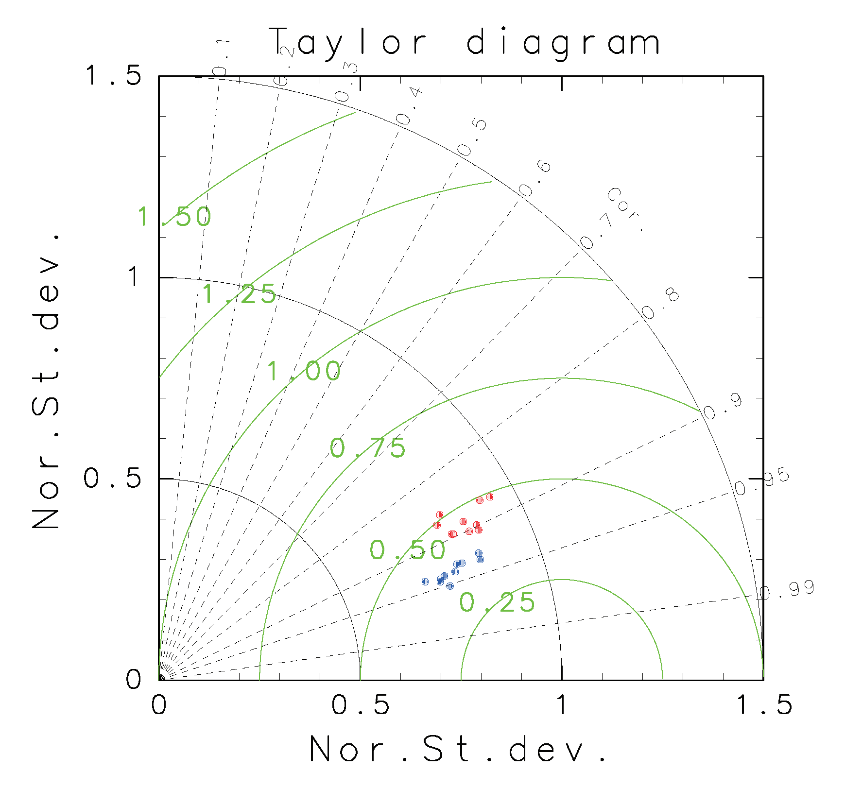
3.1. Comparison of Wave Heights

Figure 2 shows an example of significant wave heights by ERA5 and JMA. The wave heights at some of the GPS buoy locations cannot be evaluated from the ERA5 wave heights because of the low spatial resolution. The patterns of wave heights are similar to each other. However, there are some differences between them. For example, the JMA wave heights around the buoys A, B, and C are higher than those of the ERA5 wave heights.
Figure 3 shows the scatter density plots between H g and H e and between H g and H j . This figure shows the ratio of the number of wave height data in the 0.2 m bins to the total data. For example, the number of ( H g , H e ) satisfying 0.8 m ≤ H g < 1 m and 0.8 m ≤ H e < 1 m is 3222; the number of comparisons is N c = 58411 ; and the ratio is 3222 / 58411 = 5.5 % (Figure 3a). Table 1 summarizes the skill metrics of the comparison of the wave heights for each GPS buoy. The 10 GPS buoys’ data were used for the comparison. For the other eight GPS buoys, at least one of the four ERA5 grids that surround them is a land grid.
The skill metrics are R d ( H g , H e ) > R d ( H g , H j ) , r c ( H g , H e ) < r c ( H g , H j ) , and S I ( H g , H e ) > S I ( H g , H j ) for most of the buoys, except Buoy K. Thus, as explained in Section 2, the skill metrics for H j are better than those for H e . The accuracy of the JMA wave heights is better than that of ERA5 wave heights.

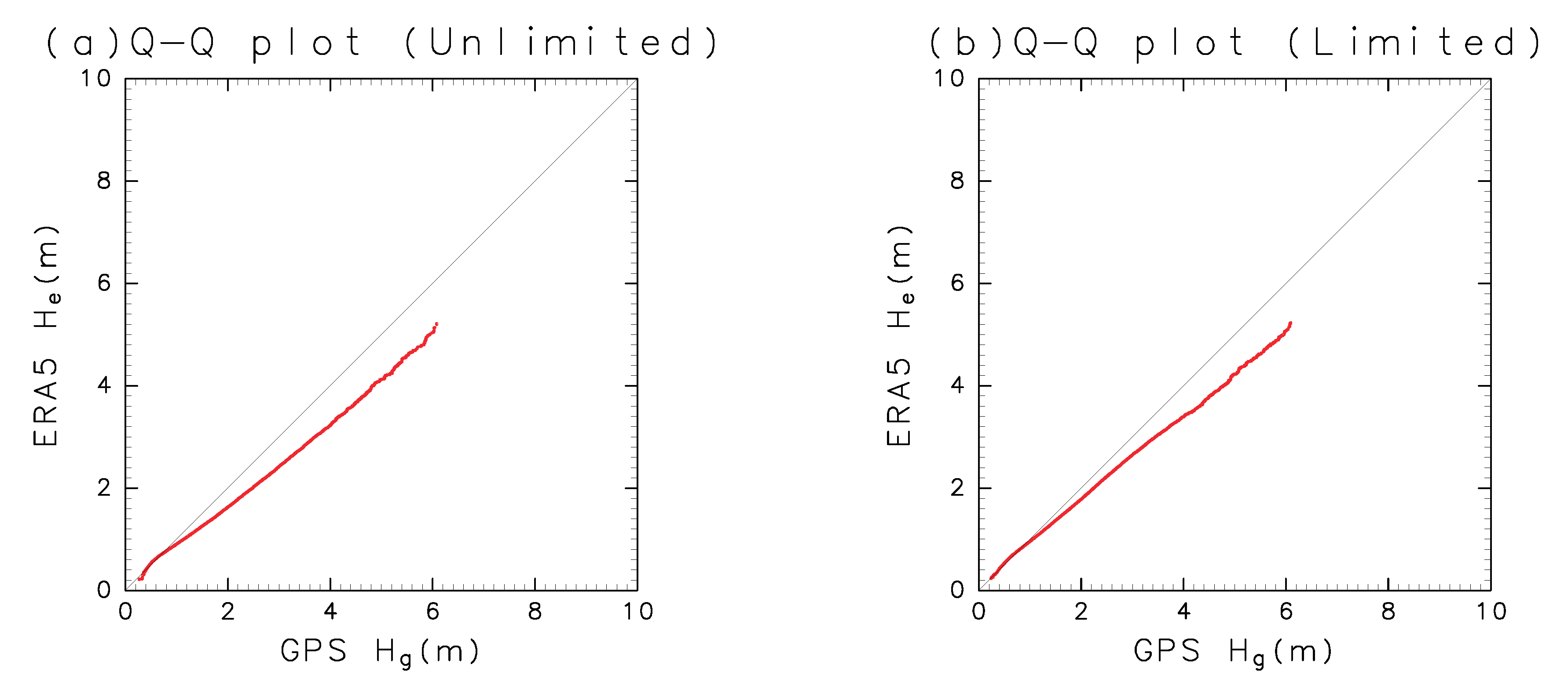
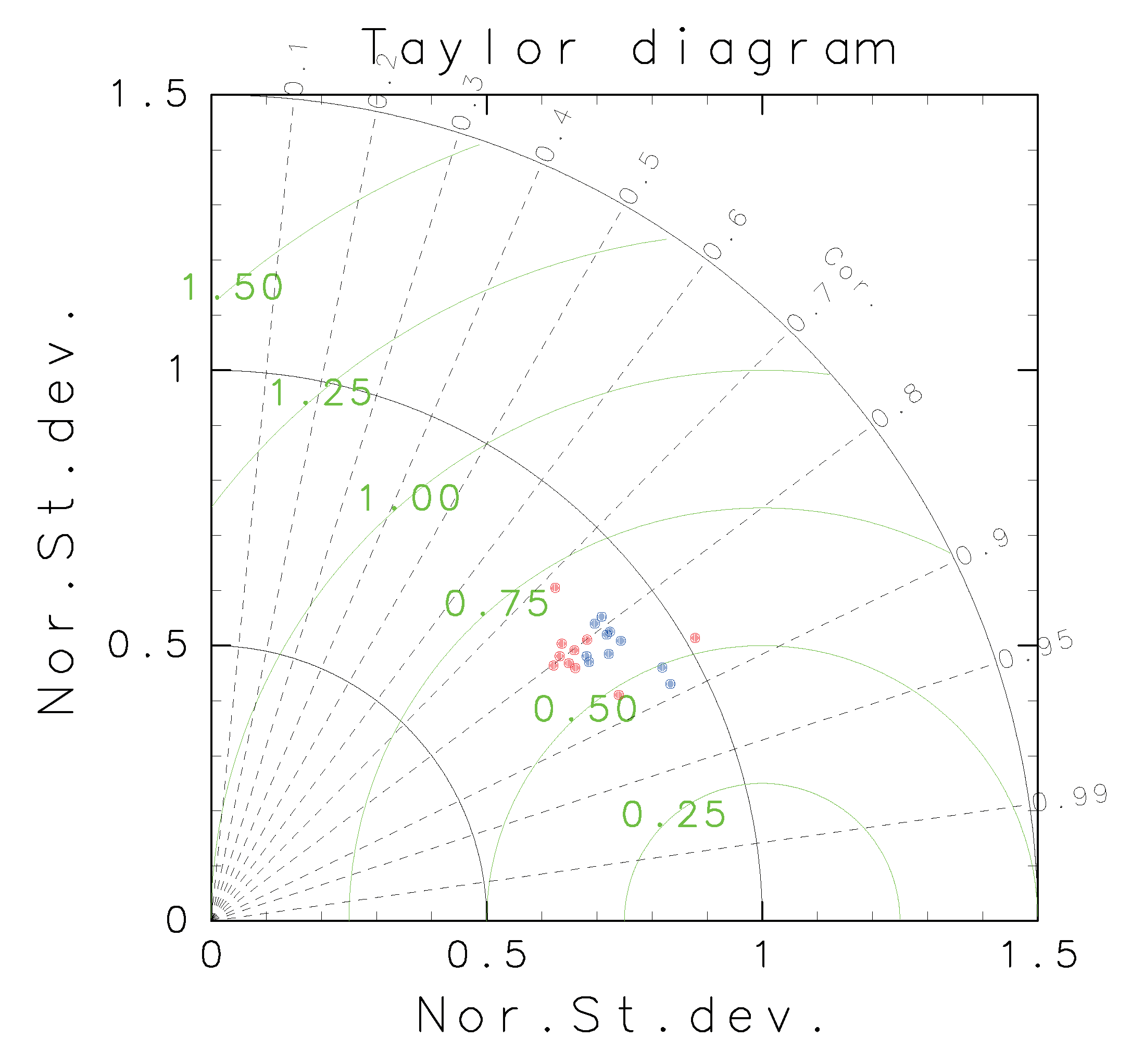
3.2. Comparison under Various Conditions

We investigated the accuracy of ERA5 and JMA wave heights with increasing wave height.
Figure 4a shows the ratios of mean wave heights ( R a ) and the CRMSD ( C r m s d ) as a function of H T for H g H T . Figure 4b shows the number of comparisons for H g H T , where H T is the threshold of wave height. For example, if H g ≥ 3 m ( H T = 3 m), R a ( H g , H e ) = 0.81 , R a ( H g , H j ) = 0.96 , C r m s d ( H g , H e ) = 0.60 , C r m s d ( H g , H j ) = 0.56 (Figure 4a), and N c = 3172 (Figure 4b). As the wave height increases, the ERA5 wave height tends to be underestimated. The CRMSD increases as the wave height increases.
Figure 5 shows the Q-Q (quantile-quantile) plots between H g and H e and between H g and H j . The ERA5 wave heights are underestimated in higher wave conditions, while the JMA wave heights are not underestimated.
The development of wind waves depends not only on the wind speed, but also on the fetch length. We investigated the accuracy of ERA5 wave heights in the fetch-unlimited condition and the fetch-limited condition. The fetch-unlimited condition and the fetch-limited condition are classified from the JMA winds ( u j , v j ) at the buoy locations. The fetch-limited conditions are u j > 0 for Buoys D, E, F, G, and J and v j < 0 for Buoys K, L, O, P, and Q (Figure 1). For example, if u j > 0 at the position of Buoy D, the fetch is limited at that time.
Figure 6 shows the Taylor diagram between H g and H e for individual buoys in the fetch-unlimited condition and in the fetch-limited condition. The data for validation are from 2012 to 2018. The plots of the fetch-unlimited condition (blue) and of the fetch-limited condition (red) are clustered with each other (Figure 6). The cluster of the fetch-unlimited condition is close to ( r c , C r m s d ) = ( 0.94 , 0.39 ) , and the cluster of the fetch-limited condition is close to ( r c , C r m s d ) = ( 0.9 , 0.5 ) . The skill indices in fetch-unlimited conditions are better than those in fetch-limited conditions except the NSD.
Table 2 summarizes the skill metrics of ERA5 wave heights in the fetch-limited condition (F) and the fetch-unlimited condition (U) for each GPS buoy. In total, R a ( H g , H e , U ) < R a ( H g , H e , F ) , r c ( H g , H e , U ) > r c ( H g , H e , F ) , R d ( H g , H e , U ) > R d ( H g , H e , F ) , C r m s d ( H g , H e , U ) < C r m s d ( H g , H e , F ) , and S I ( H g , H e , U ) > S I ( H g , H e , F ) , where R a ( H g , H e , U ) indicates R a (Equation (2)) in the fetch-unlimited condition, and R a ( H g , H e , U ) indicates R a in the fetch-unlimited condition. The same applies to other skill metrics including U and F.
The statistical significance of C r m s d ( H g , H e , U ) < C r m s d ( H g , H e , F ) , and | S s d n ( H g , H e , U ) 1 | > | S s d n ( H g , H e , F ) 1 | , which can be compared across different data groups, is explored. The bootstrap method [33,34] is used for the validation. The effective sample size N e is evaluated by the method in [33,35], which is smaller than the number of comparisons N c ( 1 N e N c ) from the serial data of ( H g , H e ) . The N e data ( H g , H e ) were resampled randomly, and they may be sampled in duplicate. The skill metrics were computed from N e data ( H g , H e ) . The resamples and computations of the skill metrics were conducted 1000 times, and the probabilities of C r m s d ( H g , H e , U ) < C r m s d ( H g , H e , F ) , and | S s d n ( H g , H e , U ) 1 | > | S s d n ( H g , H e , F ) 1 | were evaluated from 1000 resamples. This method is almost the same as those in [34,36]. The probabilities of C r m s d ( H g , H e , U ) < C r m s d ( H g , H e , F ) were greater than 95% in nine buoys out of 10 buoys. The result that the CRMSD in the fetch-unlimited case is smaller than that in the fetch-limited case is statistically significant more than at the 95% confidence level. The probabilities of | S s d n ( H g , H e , U ) 1 | > | S s d n ( H g , H e , F ) 1 | were greater than 95% in seven buoys out of 10 buoys.
Figure 7 shows the Q-Q plots between H g and H e in the fetch-limited condition and the fetch-unlimited condition. The ERA5 wave heights are underestimated as the wave height increases in both cases. Although the ratio R a ( H g , H e ) is larger in the fetch-limited condition than in the fetch-unlimited condition, the ERA5 wave heights in the fetch-limited condition are also underestimated in high wave conditions.

3.3. Comparison of Wave Periods

The comparisons of wave periods are summarized in Table 3. The correlations between peak wave periods ( T p e and T p j ) and significant wave periods ( T g = T 1 3 ) from GPS buoys are r c ( T g , T p e ) > r c ( T g , T p j ) . On the other hand, their SIs are S I ( T g , T p e ) > S I ( T g , T p j ) , but the difference is small.
The mean period T m 1 is the closest to T 1 3 in the moment periods ( T m 1 , T m 1 = M 0 / M 1 , and T m 2 = ( M 0 / M 2 ) 1 / 2 ) [37]. The value of R a ( T g , T m e ) (Equation (2)) is close to one. In total, the ERA5 mean wave periods in the fetch-unlimited conditions are closer to T g than those in the fetch-limited conditions
Figure 8 shows the Taylor diagram between T g and T m e for individual buoys in the fetch-unlimited condition and in the fetch-limited condition from 2012 to 2018. The plots are scattered compared with Figure 6. In particular, the skill metrics in the fetch-limited conditions are more scattered than those in the fetch-unlimited conditions. The CRMSDs ( C r m s d ) in the fetch-unlimited conditions tend to be smaller than those in the fetch-limited condition. The NSD ( S s d n ) in the fetch-unlimited conditions is closer to one than those in the fetch-limited condition in most of the buoys.
The probabilities of C r m s d ( T g , T m e , U ) < C r m s d ( T g , T m e , F ) and | S s d n ( T g , T m e , U ) 1 | < | S s d n ( T g , T m e , F ) 1 | are also explored by the bootstrap method. The probabilities of C r m s d ( T g , T m e , U ) < C r m s d ( T g , T m e , F ) were more than 90% in four buoys out of 10 buoys. The probabilities of | S s d n ( T g , T m e , U ) 1 | < | S s d n ( T g , T m e , F ) 1 | were more than 95% in seven buoys out of 10 buoys. The accuracy of the ERA5 wave period in the fetch-unlimited condition is better than that in the fetch-limited condition. However, the result is not so robust as wave height, because the skill metrics of wave periods are scattered (Figure 8), while the skill metrics of wave heights are clustered (Figure 6).

4. Discussion

The intercomparison of ERA5 wave data, JMA wave assimilation data, and GPS-observed wave data in the coastal area was conducted. The period of the intercomparison was from 2014 to 2018. The accuracy of wave forecast by the GWM of JMA was not good in 2013, because the wind field associated with a typhoon was not reconstructed accurately [30]. In fact, the skill metrics from 2012 to 2018 were r c ( H g , H j ) = 0.901 , R d ( H g , H j ) = 0.366 m, and S I ( H g , H j ) = 0.230 for N c = 79613 . The skill metrics of the JMA analysis wave height were lower than those in Figure 3b and Table 1.
The mean wave heights were H e < H j in all of the buoy positions (Table 1).
Figure 9 shows the mean ERA5 wind speeds and mean JMA wind speeds from 2014 to 2018. Figure 9a and Figure 9b are similar to each other. The wind speeds at the GPS buoy positions range from about 5 m/s to 7 m/s.
Figure 10 shows the differences of mean ERA5 wind speeds and mean JMA wind speeds from 2014 to 2018 ( | U j | | U e | ). The differences of mean wind speeds ( | U j | | U e | ) at the GPS buoy positions range from about 0.5 m/s to 0.3 m/s The mean wind speeds are | U j | < | U e | at five buoy positions out of 10 buoy positions. The difference of the local wind speeds cannot explain the result that H e < H j in all of the buoy positions.
GPS buoy-measured wave height data were assimilated into JMA wave data. Therefore, the accuracy of JMA wave height was better than that of ERA5. On the other hand, GPS buoy-measured wave period data were not assimilated into JMA wave data. The accuracy of JMA wave period was not better than that of ERA5.
The spatial resolution of the ERA5 wave model was 0.36 . On the other hand, the JMA model had a spatial resolution of 0.5 outside the CWM region (the CWM region is from 20 N to 50 N and from 120 E to 150 E), which was lower than that of the ERA5 wave model. It is presumed that this is because the ERA5 wave model had better reproducibility of the swell propagating from outside the CWM region. As a result, the accuracy of JMA wave period was not better than that of ERA5.
The ERA5 wave height was underestimated in higher wave conditions. The underestimation of ERA-Interim wave height in higher wave conditions was shown in [22]. This underestimation is true for ERA5 wave height.
It was found that the accuracy of ERA5 wave height was significantly different between the fetch-limited and fetch-unlimited conditions. In particular, the correlation of wave heights in fetch-limited conditions was lower than that in fetch-unlimited conditions, although the correlation cannot be compared across different data groups.
On the other hand, The ratio R a = H e / H g and NSD ( S s d n ( H g , H e ) ) were closer to one in the fetch-limited conditions than those in the fetch-unlimited conditions. The ERA5 wave heights tended to be underestimated. However, the distance between the buoy position and the coast was overestimated in the ERA5 grid (Figure 1 and Figure 2a). The fetch was overestimated at the buoy locations, and R a was larger. The normalized variability of ERA5 wave height in the fetch-limited condition was larger than that in the fetch-unlimited condition. This was also related to the overestimation of fetch in the ERA5 grid. On the other hand, the Q-Q plots in the fetch-limited condition and the fetch-unlimited condition were similar to each other. Even though the fetch was overestimated, ERA5 wave height was underestimated when the wave height was high (Figure 7).
The statistical significance of the difference of the skill metrics between the fetch-limited conditions and the fetch-unlimited conditions was investigated for each buoy’s data. The wave height changes seasonally, and the effective sample sizes N e were smaller than the number of comparisons N c . Therefore, the uncertainties of the skill metrics were large. However, the difference of the skill metrics were statistically significant at more than 90% confidence levels in most of the buoys. The uncertainties of the the skill metrics can be smaller as the data period will be extended.

5. Conclusions

The conclusions are summarized as follows:
  • The accuracy of JMA analysis wave height is better than that of ERA5 wave height by incorporating the observation data near the coast.
  • The accuracy of JMA analysis wave period is not better than that of ERA5 wave period.
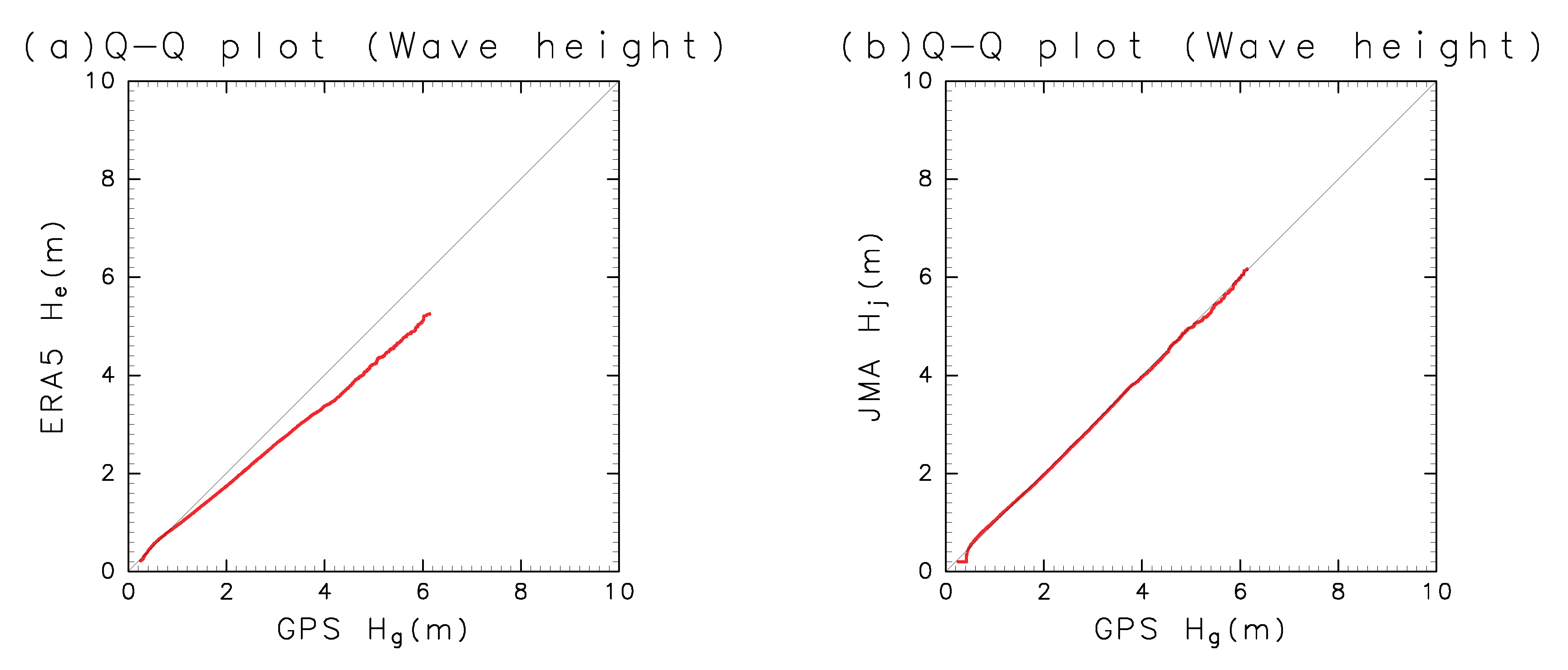
  • The ERA5 wave height is underestimated as higher wave heights.
  • The accuracy of ERA5 wave height in the fetch-limited conditions is significantly lower than that in the fetch-unlimited conditions.
  • The accuracy of ERA5 wave period in the fetch-limited conditions is also lower than that in the fetch-unlimited conditions, but this is not so robust as wave height.
From these conclusions, the JMA wave height analysis data can be used as wave climate data around Japan. In addition, if ERA5 wave data were to be used in the various marine development guidelines, ERA5 wave data should be treated separately from the fetch-limited conditions and the fetch-unlimited conditions. Moreover, since ERA5 wave heights tend to be underestimated at higher wave heights, it is necessary to pay attention to this result when using the ERA5 wave height for marine disaster prevention.

Funding

This study was financially supported by a Grant-in-Aid for Scientific Research (C-2) from the Ministry of Education, Culture, Sports, Science, and Technology of Japan (20K04708).

Acknowledgments

The GPS buoy wave data were observed by Maritime Bureau, Ministry of Land, Infrastructure, Transport, and Tourism of Japan and analyzed by the Port and Airport Research Institute. The GFD DENNOU Library (available online at http://www.gfd-dennou.org/arch/dcl/) was used for drawing the figures. Comments from the anonymous reviewers were helpful in improving the manuscript.

Conflicts of Interest

The author declares no conflict of interest.

Abbreviations

The following abbreviations are used in this paper:
ERA5Fifth generation of European Centre for Medium Range Weather Forecasting atmospheric reanalyses of the global climate
JMAJapan Meteorological Agency
ERA-InterimEuropean Centre for Medium-Range Weather Forecasts reanalysis data interim version
GPSGlobal Positioning System
CWMCoastal wave model
GWMGlobal wave model
OIOptimal interpolation
MRIMeteorological Research Institute
RMSDRoot mean squared difference
SIScatter index
CRMSDNormalized centered root mean squared difference
NSDNormalized standard deviation
Q-Q plotQuantile-quantile plot

Notations

H e ERA5 wave height.
H g GPS wave height.
H j JMA wave height.
T m e ERA5 mean wave period.
T p e ERA5 peak wave period.
T g GPS wave period.
T p j JMA peak wave period.
U j = ( u j , v j ) JMA wind vector.
U e ERA5 wind vector.
M 1 , M 0 , M 1 , M 2 Equation (1).
H s = 4 M 0 1 2 Equation (1).
H 1 3 significant wave height by the zero-up-crossing method.
T 1 3 significant wave period by the zero-up-crossing method.
T m 1 = M 0 / M 1 .
T m 1 = M 1 / M 0 .
T m 2 = ( M 0 / M 2 ) 1 / 2 .
R a ratio of averages (Equation (2)).
R d RMSD (Equation (3)).
r c correlation coefficient (Equation (4)).
C r m s d CRMSD (Equation (6)).
S s d n NSD (Equation (7)).
H T threshold of wave height.
N c number of comparisons.
N e effective sample size.

References

  1. Reguero, B.; Menéndez, M.; Méndez, F.; Mínguez, R.; Losada, I. A Global Ocean Wave (GOW) calibrated reanalysis from 1948 onwards. Coast. Eng. 2012, 65, 38–55. [Google Scholar] [CrossRef]
  2. Shi, J.; Zheng, J.; Zhang, C.; Joly, A.; Zhang, W.; Xu, P.; Sui, T.; Chen, T. A 39-year high resolution wave hindcast for the Chinese coast: Model validation and wave climate analysis. Ocean Eng. 2019, 183, 224–235. [Google Scholar] [CrossRef]
  3. Groll, N.; Weisse, R. A multi-decadal wind-wave hindcast for the North Sea 1949–2014: coastDat2. Earth Syst. Sci. Data 2017, 9, 955. [Google Scholar] [CrossRef] [Green Version]
  4. Haakenstad, H.; Breivik, O.; Reistad, M.; Aarnes, O.J. NORA10EI: A revised regional atmosphere-wave hindcast for the North Sea, the Norwegian Sea and the Barents Sea. Int. J. Climatol. 2020. [Google Scholar] [CrossRef]
  5. Shimura, T.; Mori, N. High-resolution wave climate hindcast around Japan and its spectral representation. Coast. Eng. 2019, 151, 1–9. [Google Scholar] [CrossRef]
  6. Taniguchi, K. Variations in winter ocean wave climate in the Japan sea under the global warming condition. J. Mar. Sci. Eng. 2019, 7, 150. [Google Scholar] [CrossRef] [Green Version]
  7. Hu, Y.; Shao, W.; Wei, Y.; Zuo, J. Analysis of typhoon-induced waves along typhoon tracks in the Western north Pacific Ocean, 1998–2017. J. Mar. Sci. Eng. 2020, 8, 521. [Google Scholar] [CrossRef]
  8. Chowdhury, P.; Behera, M.R. Evaluation of CMIP5 and CORDEX derived wave climate in Indian Ocean. Clim. Dyn. 2019, 52, 4463–4482. [Google Scholar] [CrossRef]
  9. Bonaduce, A.; Staneva, J.; Behrens, A.; Bidlot, J.R.; Wilcke, R.A.I. Wave climate change in the North Sea and Baltic Sea. J. Mar. Sci. Eng. 2019, 7, 166. [Google Scholar] [CrossRef] [Green Version]
  10. Li, N.; Cheung, K.F.; Stopa, J.E.; Hsiao, F.; Chen, Y.L.; Vega, L.; Cross, P. Thirty-four years of Hawaii wave hindcast from downscaling of climate forecast system reanalysis. Ocean Model. 2016, 100, 78–95. [Google Scholar] [CrossRef] [Green Version]
  11. Oliveira, B.A.; Sobral, F.; Fetter, A.; Mendez, F.J. A high-resolution wave hindcast off Santa Catarina (Brazil) for identifying wave climate variability. Reg. Stud. Mar. Sci. 2019, 32, 100834. [Google Scholar] [CrossRef]
  12. Waters, R.; Engström, J.; Isberg, J.; Leijon, M. Wave climate off the Swedish west coast. Renew. Energy 2009, 34, 1600–1606. [Google Scholar] [CrossRef]
  13. Onea, F.; Rusu, L. A long-term assessment of the Black Sea wave climate. Sustainability 2017, 9, 1875. [Google Scholar] [CrossRef] [Green Version]
  14. Saprykina, Y.; Shtremel, M.; Aydoğan, B.; Ayat, B. Variability of the Nearshore Wave Climate in the Eastern Part of the Black Sea. Pure Appl. Geophys. 2019, 176, 3757–3768. [Google Scholar] [CrossRef]
  15. Vieira, F.; Cavalcante, G.; Campos, E. Analysis of wave climate and trends in a semi-enclosed basin (Persian Gulf) using a validated SWAN model. Ocean Eng. 2020, 196, 106821. [Google Scholar] [CrossRef]
  16. Hoffmann, L.; Günther, G.; Li, D.; Stein, O.; Wu, X.; Griessbach, S.; Heng, Y.; Konopka, P.; Müller, R.; Vogel, B.; et al. From ERA-Interim to ERA5: The considerable impact of ECMWF’s next-generation reanalysis on Lagrangian transport simulations. Atmos. Chem. Phys. 2019, 19. [Google Scholar] [CrossRef] [Green Version]
  17. Hersbach, H.; Bell, B.; Berrisford, P.; Hirahara, S.; Horányi, A.; Muñoz-Sabater, J.; Nicolas, J.; Peubey, C.; Radu, R.; Schepers, D.; et al. The ERA5 global reanalysis. Q. J. R. Meteorol. Soc. 2020. [Google Scholar] [CrossRef]
  18. Kohno, N.; Miura, D.; Yoshita, K. The development of JMA wave data assimilation system. In Proceedings of the 12th International Workshop on Wave Hindcasting and Forecasting, Kona, HI, USA, 30 October–4 November 2011; pp. 1–8. Available online: http://www.waveworkshop.org/12thWaves/papers/full_paper_Kohno_et_al.pdf (accessed on 31 July 2020).
  19. Pastor, J.; Liu, Y.; Dou, Y. Wave energy resoruce analysis for use in wave energy conversion. J. Offshore Mech. Arct. Eng. 2015, 137, 011903-1. [Google Scholar]
  20. Guiberteau, K.L.; Liu, Y.; Lee, J.; Kozman, T. Potential of Development and Application of Wave Energy Conversion Technology in the Gulf of Mexico; Energy Systems Laboratory: New Orleans, LA, USA, 2014; pp. 132–141. [Google Scholar]
  21. Pastor, J.; Liu, Y. Wave climate resource analysis based on a revised gamma spectrum for wave energy conversion technology. Sustainability 2016, 8, 1321. [Google Scholar] [CrossRef] [Green Version]
  22. Stopa, J.E.; Cheung, K.F. Intercomparison of wind and wave data from the ECMWF Reanalysis Interim and the NCEP Climate Forecast System Reanalysis. Ocean Model. 2014, 75, 65–83. [Google Scholar] [CrossRef]
  23. Campos, R.; Soares, C.G. Comparison of HIPOCAS and ERA wind and wave reanalyses in the North Atlantic Ocean. Ocean Eng. 2016, 112, 320–334. [Google Scholar] [CrossRef]
  24. Sanil Kumar, V.; Muhammed Naseef, T. Performance of ERA-Interim wave data in the nearshore waters around India. J. Atmos. Ocean. Technol. 2015, 32, 1257–1269. [Google Scholar] [CrossRef]
  25. Shanas, P.; Kumar, V.S. Temporal variations in the wind and wave climate at a location in the eastern Arabian Sea based on ERA-Interim reanalysis data. Nat. Hazards Earth Syst. Sci 2014, 14, 1371–1381. [Google Scholar] [CrossRef] [Green Version]
  26. Bruno, M.F.; Molfetta, M.G.; Totaro, V.; Mossa, M. Performance Assessment of ERA5 wave data in a swell dominated region. J. Mar. Sci. Eng. 2020, 8, 214. [Google Scholar] [CrossRef] [Green Version]
  27. Sifnioti, D.; Dolphin, T.; Vincent, C. Performance of Hindcast Wave Model Data used in UK Coastal Waters. J. Coast. Res. 2020, 95, 1284–1290. [Google Scholar] [CrossRef]
  28. Muhammed Naseef, T.; Sanil Kumar, V. Climatology and trends of the Indian Ocean surface waves based on 39-year long ERA5 reanalysis data. Int. J. Climatol. 2020, 40, 979–1006. [Google Scholar] [CrossRef]
  29. Ueno, K.; Kohno, N. The development of the third generation wave model MRI-III for operational use. In Proceedings of the 8th International Workshop on Wave Hindcasting and Forecasting, North Shore, HI, USA, 14–19 November 2004; Available online: http://www.waveworkshop.org/8thWaves/Papers/G2.pdf (accessed on 31 July 2020).
  30. JMA. Outline of the Operational Numerical Weather Prediction at the Japan Meteorological Agency. 2019. Available online: https://www.jma.go.jp/jma/jma-eng/jma-center/nwp/outline2019-nwp/index.htm (accessed on 31 July 2020).
  31. Kawaguchi, K.; Inomata, T.; Seki, K.K.; Fujiki, T. Annual Report on Nationwide Ocean Wave Information Network for Ports and Harbours (NOWPHAS 2012); Port and Airport Research Institute Technical Note; Port and Airport Research Institute: Yokosuka, Japan, 2014; Available online: https://www.pari.go.jp/search-pdf/no1282.pdf (accessed on 31 July 2020).
  32. Goda, Y. Random Seas and Design of Maritime Structures; World Scientific Publishing Company: Singapore, 2010; Volume 33. [Google Scholar] [CrossRef]
  33. Emery, W.J.; Thomson, R.E. Data Analysis Methods in Physical Oceanography; Pergamon: İzmir, Turkey, 1998. [Google Scholar]
  34. Hisaki, Y. Wave hindcast in the North Pacific area considering the propagation of surface disturbances. Prog. Oceanogr. 2018, 165, 332–347. [Google Scholar] [CrossRef]
  35. Trenberth, K.E. Some effects of finite sample size and persistence on meteorological statistics. Part II: Potential predictability. Mon. Weather Rev. 1984, 112, 2369–2379. [Google Scholar] [CrossRef] [Green Version]
  36. Hisaki, Y. Sea surface wind correction using HF ocean radar and its impact on coastal wave prediction. J. Atmos. Ocean. Technol. 2017, 34, 2001–2020. [Google Scholar] [CrossRef]
  37. Yamaguchi, M.; Nonaka, H. Effect of Spectral Form on the Ratio between Surface Elevation-Based Statistics and Spectrum-Based Statistics of Wave Height and Wave Period. J. Jpn. Soc. Civ. Eng. Ser. B2 (Coast. Eng.) 2009, 65, 136–140. (In Japanese) [Google Scholar] [CrossRef]
Figure 1. Locations of the moored GPS buoys (A–R). Black squares: land grid points on ERA5 grids.
Jmse 08 00579 g001
Figure 2. Example of (a) ERA5 wave height and (b) JMA wave height at 18 UT 1 January 2018.
Jmse 08 00579 g002
Figure 3. Scatter density plots (a) between H g and H e and (b) between H g and H j in the 0.2 m bins. The line indicates linear regression. The period of the comparison is from 2014 to 2018. SI, scatter index.
Jmse 08 00579 g003
Figure 4. (a) Ratios of mean wave heights ( R a ) and the centered RMSD (CRMSD) ( C r m s d ) as a function of H T and (b) the number of data for comparison, which satisfies H g H T . (a) Black: R a ( H g , H e ) (Equation (2)). Blue: R a ( H g , H j ) . Red: C r m s d ( H g , H e ) (Equation (6)). Green: C r m s d ( H g , H j ) . The period of the comparison is from 2014 to 2018.
Jmse 08 00579 g004
Figure 5. (a) Q-Q plots (from 0.1 to 99.9%) between H g and H e . Same for (b), but between H g and H j . The period of the comparison is from 2014 to 2018.
Jmse 08 00579 g005
Figure 6. Taylor diagram between H g and H e for individual buoys in the fetch-unlimited condition (blue) and in the fetch-limited condition (red). The black arcs show normalized standard deviation (NSD) contours, and the green arcs show CRMSD contours. The period of the comparison is from 2012 to 2018.
Jmse 08 00579 g006
Figure 7. (a) Q-Q plots (from 0.1 to 99.9%) between H g and H e in the fetch-unlimited condition Same for (b) in the fetch-limited condition. The period of the comparison is from 2012 to 2018.
Jmse 08 00579 g007
Figure 8. Same as Figure 6, but for between T g and T m e . The period of the comparison is from 2012 to 2018.
Jmse 08 00579 g008
Figure 9. (a) Mean ERA5 wind speeds from 2014 to 2018 ( | U e | ). (b) Same as (a), but for JMA wind speed ( | U j | ).
Jmse 08 00579 g009
Figure 10. Differences of mean ERA5 wind speeds and mean JMA wind speeds from 2014 to 2018 ( | U j | | U e | ).
Jmse 08 00579 g010
Table 1. Comparison of H g ( X = H g ) with H e and H j ( Y = H e or Y = H j ) for various buoys from 2014 to 2018. N c : number of comparisons. Other symbols are defined in Equations (2)–(6).
BuoyY X (m) Y (m) R a r c R d (m)SI C rmsd S sdn N c
D H e 1.4731.3920.9450.8840.3710.2460.4700.8497197
D H j 1.4731.4971.0160.9270.2900.1960.3760.9617197
E H e 1.6661.3810.8290.9070.4550.2130.4410.7797179
E H j 1.6661.6000.9600.9460.2690.1560.3240.9547179
F H e 1.6971.4490.8540.9110.4270.2050.4290.7927124
F H j 1.6971.6690.9830.9440.2710.1590.3320.9667124
G H e 1.6241.4250.8770.8920.4330.2360.4670.7736842
G H j 1.6241.6421.0110.9390.2840.1740.3450.9536842
J H e 1.7221.5240.8850.9130.3860.1920.4140.8377184
J H j 1.7221.6570.9620.9210.3200.1820.3910.9647184
K H e 1.7391.4710.8460.9100.4460.2050.4180.8563847
K H j 1.7391.6830.9680.8830.4100.2330.4750.9503847
L H e 1.1931.1620.9740.8990.3050.2540.4440.8284344
L H j 1.1931.5161.2700.9150.4410.2520.4401.0914344
O H e 1.3411.2470.9300.9040.3430.2460.4290.8655263
O H j 1.3411.3060.9740.9100.3350.2490.4331.0385263
P H e 1.4081.4331.0170.9180.3460.2450.4000.8665637
P H j 1.4081.5521.1020.9280.3580.2330.3801.0015637
Q H e 1.6081.4820.9220.8920.4410.2630.4590.8133794
Q H j 1.6081.6331.0150.9330.3330.2060.3600.9553794
Total H e 1.5601.4020.8990.8990.4000.2360.4450.81558,411
Total H j 1.5601.5781.0120.9210.3250.2080.3930.96658,411
Table 2. Comparisons between H g and H e in the fetch unlimited conditions (U) and the fetch-limited conditions (F) for various buoys from 2012 to 2018. The asterisk (*) denotes that the probability that C r m s d ( H g , H e , U ) < C r m s d ( H g , H e , F ) ( | S s d n ( H g , H e , U ) 1 | > | S s d n ( H g , H e , F ) 1 | is less than that in the fetch-limited condition is greater than 95%. The asterisks (**) denote the probability is greater than 90%, but less than 95%.
BuoyCase H g (m) H e (m) R a r c R d (m)SI C rmsd S sdn N c
DU1.5371.3090.8520.9390.3990.2130.389 *0.7553656
DF1.4381.4511.0090.8750.3430.2380.4890.939 *5752
EU1.6681.2870.7720.9380.5160.2090.418 *0.7044380
EF1.7221.4820.8600.8960.4340.2090.4520.816 *5667
FU1.6931.3830.8170.9440.4520.1940.388 *0.7404003
FF1.7401.5180.8720.8950.4320.2130.4540.812 *5985
GU1.7411.4240.8180.9410.4660.1970.392 *0.7433163
GF1.5971.4480.9070.8730.4290.2520.4940.790 *6254
JU1.8031.5170.8410.9330.4240.1730.382 *0.8064251
JF1.7121.5460.9030.9020.3870.2040.4350.854 *5816
KU1.4821.3020.8780.9290.3750.2220.377 **0.8542698
KF1.9481.5860.8140.8980.5040.1800.4400.8784048
LU1.1931.0620.8910.9510.3120.2370.363 *0.7601858
LF1.1981.2121.0120.8870.3110.2600.4630.852 *3216
OU1.4101.2500.8860.9390.3720.2380.378 *0.7832697
OF1.3311.2280.9230.8720.3550.2550.4910.913 *4284
PU1.4001.4281.0200.9360.3350.2380.361 *0.8522115
PF1.4131.4361.0160.9050.3520.2490.4260.8773522
QU1.6181.4020.8670.9320.4230.2250.389 *0.7942542
QF1.5431.4680.9510.8610.4520.2890.5110.8093706
TotalU1.5931.3500.8480.9310.4240.2180.3980.77231363
TotalF1.5861.4500.9140.8820.4060.2410.4740.83348250
Table 3. Comparison of periods ( X = T g , Y = T p e , or Y = T p j , or Y = T m e ). T: total. U: fetch-unlimited conditions. F: fetch-limited conditions. Other symbols are defined in Equations (2)–(6). The comparison period with T p e , T p j , and T m e for the total cases (T) is from 2014 to 2018. The comparison period with T m e for the fetch-unlimited (U) and the fetch-limited (F) cases is from 2012 to 2018.
YCase X (s) Y (s) R a r c R d (s)SI C rmsd S tdn N c
T p e T7.3018.9101.2200.6712.3760.2391.0191.37058,411
T p j T7.3018.7021.1920.6102.2160.2351.0001.22158,411
T m e T7.3017.3201.0030.8001.0380.1420.6050.87258,411
T m e U7.5037.5401.0050.8010.9790.1300.6060.89732,044
T m e F7.1907.1500.9940.7921.0930.1520.6120.83347,561

