Development of Deterministic Artificial Intelligence for Unmanned Underwater Vehicles (UUV)

Abstract

The major premise of deterministic artificial intelligence (D.A.I.) is to assert deterministic self-awareness statements based in either the physics of the underlying problem or system identification to establish governing differential equations. The key distinction between D.A.I. and ubiquitous stochastic methods for artificial intelligence is the adoption of first principles whenever able (in every instance available). One benefit of applying artificial intelligence principles over ubiquitous methods is the ease of the approach once the re-parameterization is derived, as done here. While the method is deterministic, researchers need only understand linear regression to understand the optimality of both self-awareness and learning. The approach necessitates full (autonomous) expression of a desired trajectory. Inspired by the exponential solution of ordinary differential equations and Euler’s expression of exponential solutions in terms of sinusoidal functions, desired trajectories will be formulated using such functions. Deterministic self-awareness statements, using the autonomous expression of desired trajectories with buoyancy control neglected, are asserted to control underwater vehicles in ideal cases only, while application to real-world deleterious effects is reserved for future study due to the length of this manuscript. In totality, the proposed methodology automates control and learning merely necessitating very simple user inputs, namely desired initial and final states and desired initial and final time, while tuning is eliminated completely.

1. Introduction

Artificial intelligence is most often expressed in stochastic algorithms that often have no knowledge whatsoever of the underlying problem being learned (a considerable strength of the methods). The field of non-stochastic or deterministic artificial intelligence breaks from this notion by first asserting the nature of the underlying problem using a self-awareness statement that permits the controlled item to have knowledge of itself, and this assertion allows the controlled item to learn in reaction to the environment. Thus, an unmanned vehicle with a deterministic self-awareness and learning can respond to significant damage that removes substantial vehicle parts or instead increases the vehicle’s math models via inelastic collisions (e.g., bird strikes on aircraft, or robotic capture for spacecraft and underwater vehicles).

It is sometimes said that science fiction can be a precursor to science-fact, and such it is with artificial intelligence [1] vis-à-vis Karel Čapek’s Rossum’s Universal Robots and Frankenstein by Mary Shelley [2]. Ethical issues of artificial intelligence were first grappled with in such fictional works [1]. As ancient mathematicians and philosophers studied reasoning formally, computation as a theory emerged, embodied in the Church-Turing thesis suggesting that any mathematical action could be represented digitally by combinations of zeros and ones [3], where “intelligence” was defined as the ability for these mathematical actions being indistinguishable from human responses [4]. In 1943, Pitts and McCullouch formalized Turing’s design, whose artificial neurons instantiated artificial intelligence [5]. In 1956, Dartmouth College hosted a summer workshop [6] attended by A.I. pioneers IBM’s Arthur Samuel, MIT’s Marvin Minsky and John McCarthy, and Carnegie-Mellon’s Herbert Simon and Allen Newell [2]. The result was computer programs that learned checkers strategies [2], and within four years [7], these programs were better than average humans [8]. Logical Theorems were proved in the computers’ ability to solve algebra word problems and speaking English [2]. Artificial intelligence research subsequently launched in earnest following considerable monetary support by the U.S. defense department [9], but was not limited to the United States [10]. An original Dartmouth summer workshop attendee from MIT, Marvin Minsky, was so enthusiastic to state in writing, “within a generation … the problem of creating ‘artificial intelligence’ will substantially be solved” [9,11,12], clearly failing to acknowledge some very difficult challenges.

Sir James Lighthill’s critique [13] of the early 1970s exemplifies the admission of the lost potential realized by the de-funding of artificial intelligence research by Britain and American governments, demarking a time-period of artificial intelligence research drought [5,9,10,14,15]. Seeking to develop artificially intelligent systems mimicking human experts’ knowledge and analytical skills, a billion-dollar commercial sector substantially launched in the 1980s [1,2,9,14,15,16,17]. Research by academia was shortly salvaged by re-initiation of government support to compete for honor in the face of the support by Japan [1,2,9,16], but a longer drought immediately followed in the late 1980s [1,9,16,17]. By the 1990s, other research [18] presented logic, rule, object and agent-based architectures, along with example programs written in LISP and PROLOG. Accompanying continual computation evolution often referred to as “Moore’s Law,” artificial intelligence was afterwards adopted for statistics and mathematics, data mining, economics, medicine, and logistics [2,16,17,19], leading to the adoption of standards [1,2] An IBM company artificial intelligence system easily beat two of the best players at the TV show Jeopardy in 2011 [20], and by 2012, so-called deep-learning methods became the most accurate instantiations [21]. Currently, artificial intelligence algorithms are used every day in smart phones and video game consoles such as Xbox [22,23], and even the abstract strategy board game Go [24,25,26,27,28]. Shortly thereafter, the search-engine giant Google had, by 2015, nearly 3000 artificial intelligence software projects, while the maturity of artificial intelligence was documented in Bloomberg vis-à-vis low image processing error rates attributable to cost reduction of neural networks accompanying the significant expansion of infrastructure for cloud computing and proliferation of data sets and tools for research [29]. Image processing error improvements led the social media company Facebook to develop a system to describe images to the blind, while Microsoft enhanced their Skype telecommunication software with artificial intelligent language translation abilities [29]. Twenty percent of companies surveyed in 2017 used artificial intelligence in some form [30,31] amidst increased government funding in China [32,33]; however, it must be elaborated that in a modern continuation of the original exaggeration in the 1960s and 1970s of the abilities of artificial intelligence, current reporting has also been established as exaggerated [34,35,36].

In order to statistically maximize success likelihood, artificial intelligent systems continually analyze their environment [2,15,37,38], while induced or explicit goals are expressed by figures of merit often referred to as a utility function, which can be quite complex or quite simple. Utility functions in deterministic systems are sometimes referred to as cost functions, where the cost is pre-selected and subsequently maximized or minimized to produce the deterministic form of the best behavior similarly to how animals evolved to innately possess goals such as finding food [39]. Some systems, such as nearest-neighbor are non-goal systems framed as systems whose “goal” is to successfully accomplish its narrow classification task [40].

The goal pursued in the proposed deterministic artificial intelligence approach will be the elimination of motion trajectory tracking error (and do so in an optimal manner), and therefore, the approach will seek to exactly track unknown or arbitrary user commands, and learning will be performed on truly unknowable parameters that are typically assumed to be reasonable constants in classical linear, time-invariant (LTI) methods. The physical system will be an autonomously piloted (without human intervention) underwater robotic vehicle that has already been well-studied by classical methods [41]. Improvement over the most recent investigation of classical methods [42] was proposed to and funded by the U.S. Office of Naval Research, where the winning proposal [43] contained two parts: deterministic artificial intelligence methods and non-propulsive maneuvering by momentum exchange stemming from a recent lineage [44,45,46,47,48,49,50,51]. While the former is the subject of this manuscript, the latter is neglected here (reserved for a future manuscript).

While most artificial intelligence methods are stochastic, emerging deterministic artificial intelligence (not to be confused with deterministic algorithms [52] or deterministic environments [53]) ignores articulated uncertainty, preferring instead to determine the analytic relationship that minimizes uncertainty (e.g., so-called two-norm optimization among others). Therefore, a key challenge is re-parameterization of the underlying problem into a form that permits such optimization to minimize variance and/or uncertainty.

Thus, a key novel contribution of this manuscript is re-parameterization, in addition to the illustration of optimality and validation of basic performance. Autonomous trajectory generation accepting arbitrary user commands and outputting statements of desired full state trajectories will be adopted and elaborated from the very recent literature [54], while parameter modification and disturbance formulation will similarly adopt the most current methods [55]. Taking these new developments for granted, the remaining task addressed in this manuscript will be accomplished by asserting physics-based [56,57,58] mathematical deterministic self-awareness statements, while learning will be developed using simple methods (stemming from a heritage in adaptive systems) [59,60,61,62,63,64,65,66,67,68,69,70,71,72,73,74,75,76,77,78,79] and also new optimal methods embodying the aforementioned reparameterization seeking 2-norm error minimization learning. [59,60,61] describe use of mathematic models are references, where adaption rules are invoked to make the system behave like the chosen model. [61,62,63,64,65,66] articulate methods of identifying system models from data of performance for various systems, rather than invocation of preferred reference models. References [67,68,69,70,71,72,73] utilize data-derived models in the various adaptive schemes, while [74] substantiates the first evolution from simple adaptive systems with the innovation of deterministic self-awareness applied to the forced van der Pol equation. References [75,76,77,78] illustrate the utilization of the system models towards optimization and prediction. Lastly, [79] is the first book devoted to the application of the methods developed here applied to space systems, while this manuscript applies the methods to underwater vehicles. Care is taken to cite the original source of the inspiring first principle relationships for deterministic self-awareness statements in addition to the references of subsequent expansion and eventual application to deterministic self-awareness.

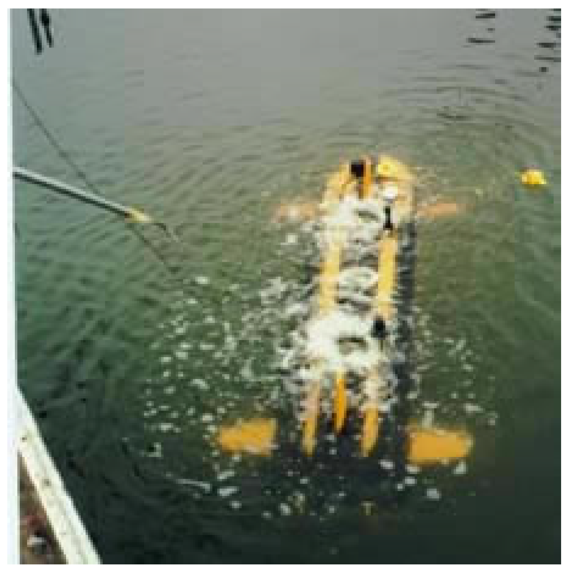
Why Use the Proposed Approach on a UUV?

One instance to consider using deterministic artificial intelligence (D.A.I.) is where the users strictly need autonomous operations, since the method is developed to make the Unmanned Underwater Vehicles (UUVs) depicted in Figure 1 self-aware with learning mechanisms that permit the UUV to autonomously operate (a goal shared with common robotics and controls methods), but also understand its performance in terms of its mathematical model leading to an ability to self-correct, but also to self-diagnose problems and notify land-based or ship-based infrastructure details of the vehicle’s dynamic models.

Another reason to consider using D.A.I. for UUVs lies in the elimination of the necessity for backgrounds in robotics and/or controls, substituting instead with a prerequisite understanding of (1) dynamics and (2) regression. In model predictive control [75,76,77], the dynamics are used to predict system behavior, which is compared to the behavior of a desired (simpler) dynamic model, and the difference between the two is used to formulate a control that seeks to drive the actual dynamic behavior to mimic the behavior of the desired dynamic. Reference [76] also highlights a very realistic issue: actuator saturation and under actuation (driven by hardware selection). This motivates the final sections of this manuscript: an implementable operational procedure that starts with a selection of actuators, and uses their limits to determine the desired maneuver times for the autonomous trajectory generation scheme, which feeds the D.A.I. calculations.

With D.A.I, the dynamics comprise the self-awareness statements (albeit necessitating the articulation of desired trajectories). This assertion of the dynamics stems from the physics-based control methods [56,57,58], which was proven to eliminate lag in references [58,67]. Such assertion is also shared with the field of nonlinear adaptive control [69,70,71,72,73], while the feedback is typically of the classical type (utilizing proportional, derivative, and sometimes integral actions). The use of feedback in the form of learning presented here neglects these classical forms, separating the method from the nonlinear adaptive control. Other forms of adaptive control and system identification (e.g., auto-regressive moving average parameterization, among others) do not parameterize the problem in terms of the dynamics, as presented in [62,63,64,65,66]. One key development illustrating the powerful idea of asserting the dynamics as self-awareness statements comes in a research by Cooper et al. [74], who eliminated feedback altogether in the control of the forced van der Pol equation. Other approaches emphasizing the use of the dynamics include real-time optimal control as compared in [75] to several other approaches, including classical feedforward plus feedback, open-loop optimal control and also predictive control. Offline nonlinear optimization [78] also emphasizes use of the dynamics, but adjoins the dynamics and constraints with a cost function to numerically find trajectories and controls that minimize the combined adjoined cost function. This use of the dynamics is effective but relatively unwieldy compared to the analytic approach developed here.

2. Materials and Methods

Deterministic artificial intelligence (D.A.I.) requires a self-awareness (mathematical) statement derived from the governing physics followed by some type of learning (either stochastic or deterministic). The deterministic self-awareness statement requires the creation of a desired state trajectory, and rather than demand offline work by a designing engineer, the first section of this section of the manuscript introduces one potential online autonomous (desired) trajectory generation scheme. Afterwards, the deterministic self-awareness statement will be introduced neglecting standard kinematic representations [80] in favor or recent expressions for UUVs [42], followed by two approaches to learning: simple learning, and optimal learning. Each component of D.A.I. will be elaborated in sufficient detail to allow the reader to replicate the published results and use the methods on systems not elaborated in this document. Graphic images of systems coded in MATLAB/SIMULINK (depicted in Figure 2) will aid the reader in creating their own validating simulations. For the sake of easier reading, variable definitions are provided in each section where the reader will be introduced to the variables, while a summary table of all variable definitions is provided in the Appendix A.

2.1. Deterministic Artificial Intelligence Self-Awareness Statement

In a two-step process, first impose the governing equations of motion expressing the dominant physics of the problem as the deterministic artificial intelligence self-awareness statement. The second step will be to assert these governing equations using “desired trajectories.” Rearranging the equations allows expression in the so-called state-space form ubiquitously associated with modern control methods, a very well-articulated topic [81,82,83,84,85]. Subsequently (in the next section of this manuscript), the self-awareness statement(s) will be reparametrized to isolate variables that are to be learned (in this instance: center of gravity, masses, and mass moments of inertia); first using simple learning algorithms, then using optimal learning methods. Items that possess mass behave in accordance with several first principles, among them Hamilton’s Principle [86], the conservation of energy or of momentum [87,88,89,90,91] and angular momentum [92,93,94,95], Lagrange’s equations [96], Kane’s Method [97,98,99,100], and Newton’s Law [101] together with Euler’s equations [102,103,104,105,106,107], which may be invoked in accordance with Chasle’s theorem [108], while invocation motivates the assertion of the dynamic equations as deterministic self-awareness statements. The dynamics of unmanned underwater vehicles, per the defining components of dynamics comprises kinetics in Equations (1)–(6) and kinematics, and these are expressed in Equations (7)–(11). As equations are developed small “mini tables” of acronyms are provide in

Table 1. Definitions of variables in this part of the manuscript (while a consolidated list is provided in the Appendix A).

Nondimensional Variable	Definition
$m$	Mass
$x_G$	Position of center of mass in meters
$I_z$	Mass moment of inertia with respect to a vertical axis that passes through the vehicle’s geometric center (amidships)
$\nu$,$\dot{\nu }$	Lateral (sway) velocity and rate
$\psi$,$\dot{\psi }$	Heading angle and rate
$x,y,\dot{x},\dot{y}$	Cartesian position coordinates and derivatives
$z,\dot{z},\ddot{z}$	Dummy variables and derivatives for generic motion states
$A,A_0,\lambda$	Dummy variables for final and initial amplitude and eigen variable in exponential solution of ordinary differential equations
$\omega ,t,T$	Sinusoidal frequency and time variables
$z,\dot{z},\ddot{z}$	Dummy variables and derivatives for generic motion states
$r$	Turning rate (yaw)
${\delta }_s$,${\delta }_s^{*}$	Deflection of stern rudder and its optimal variant
${\delta }_b$,${\delta }_b^{*}$	Deflection of bow rudder and its optimal variant
$Y_r,Y_{\dot{r}},Y_{\nu },Y_{\dot{\nu }}$,$Y_{{\delta }_s},Y_{{\delta }_b}$	Sway force coefficients: coefficients describing sway forces from resolved lift, drag, and fluid inertia along body lateral axis. These occur in response to individual (or multiple) velocity, acceleration and plane surface components, as indicated by the corresponding subscripts
$N_{{\delta }_s},N_{{\delta }_b}$,$N_r,N_{\dot{r}}$,$N_{\nu },N_{\dot{\nu }}$	Yaw moment coefficients
${\mathrm{₵}}_i\forall i{{\displaystyle \cap }}^{}\left(1\dots 8\right)$	Arbitrarily labeled constants used to simplify expressions
${\mathrm{₵}}_{u_1}\forall i{{\displaystyle \cap }}^{}\left(1\dots 2\right)$

Variable found ubiquitously throughout Equations (1)–(52), but this reduced list aids readers follow proximal Equations (1)–(21) [41].

,

Table 2. Definitions of variables in this part of the manuscript (while a consolidated list is provided in the Appendix A).

Variable	Definition
$z$,$\dot{z},\ddot{z}$	Arbitrary motion states (position, velocity, and acceleration) variables used to formulate autonomous trajectories
$A$, $A_o$	Arbitrary motion state displacement amplitude and initial amplitude used to formulate autonomous trajectories
$\lambda$	Eigenvalue associated with exponential solution to ordinary differential equations
$\omega$	Frequency of sinusoidal functions
$t$	Time
$\varphi$	Phase angle of sinusoidal functions
$T$	Period of sinusoidal functions
$\mathrm{\Delta }{t}_{quiescant}$	User-defined quiescent period used to trouble-shoot and validate computer code (no motion should occur during the quiescent period).
$\mathrm{\Delta }{t}_{maneuver}$	User-defined duration of maneuver (often established by time-optimization problems)

Variable found ubiquitously throughout Section 2.2.

and

Table 3. Definitions of variables in this part of the manuscript (while a consolidated list is provided in the Appendix A).

Variable	Definition
$a_1,a_2,a_3,a_4$	Variables in state-variable formulation (“state space”) of equations of motion associated with motion states
$b_1,b_2,b_3,b_4$	Variables in state-variable formulation (“state space”) of equations of motion associated with controls
${\delta }_s^{*}$	Deterministic error-optimal stern rudder displacement commands
${\delta }_b^{*}$	Deterministic error-optimal bow rudder displacement commands
$\widehat{m}$	Learned vehicle mass
$\widehat{m{x}_G}$	Learned product of vehicle mass and location of center of mass
$\widehat{x_G}$	Learned location of center of mass
${\widehat{I}}_Z, {\widehat{I}}_Z{}_0$	Learned mass moment of inertia and initial value
$K_{m_1}$	Control gain for mass simple-learning
$K_{m{x}_G{}_1}$	Control gain for learning product of mass and location of center of mass
$K_{I_1}$,$K_{I_2}$	Control gain for learning mass moment of inertia
${\mathrm{₵}}_i^{*}\forall i{{\displaystyle \cap }}^{}\left(1\dots 6\right)$	Variables (combinations of motion states) used to reparametrize problem into optimal learning form

Superscript “$\widehat{}$” indicates quantities estimated by learning or feedback in Equations (1)–(52), but this reduced list aids readers to follow proximal Equations (22)–(52).

to aid readability without continually flipping back and forth between pages, while a complete “summary table” of acronyms is provided in the Appendix A in

Table A1. Consolidated table of variable definitions.

Nondimensional Variable	Definition
$m$	Mass
$x_G$	Position of center of mass in meters
$I_z$	Mass moment of inertia with respect to a vertical axis that passes through the vehicle’s geometric center (amidships)
$\nu$,$\dot{\nu }$	Lateral (sway) velocity and rate
$\psi$,$\dot{\psi }$	Heading angle and rate
$x,y$	Cartesian position coordinates
$r$	Turning rate (yaw)
${\delta }_s$,${\delta }_s^{*}$	Deflection of stern rudder and its optimal variant
${\delta }_b$,${\delta }_b^{*}$	Deflection of bow rudder and its optimal variant
$Y_r,Y_{\dot{r}},Y_{\nu },Y_{\dot{\nu }}$,$Y_{{\delta }_s},Y_{{\delta }_b}$	Sway force coefficients: coefficients describing sway forces from resolved lift, drag, and fluid inertia along body lateral axis. These occur in response to individual (or multiple) velocity, acceleration, and plane surface components, as indicated by the corresponding subscripts
$N_{{\delta }_s},N_{{\delta }_b}$,$N_r,N_{\dot{r}}$,$N_{\nu },N_{\dot{\nu }}$	Yaw moment coefficients
${\mathrm{₵}}_i\forall i{{\displaystyle \cap }}^{}\left(1\dots 8\right)$	Arbitrarily labeled constants used to simplify expressions
${\mathrm{₵}}_{u_1}\forall i{{\displaystyle \cap }}^{}\left(1\dots 2\right)$
$z$,$\dot{z},\ddot{z}$	Arbitrary motion states (position, velocity, and acceleration) variables used to formulate autonomous trajectories
$A$, $A_o$	Arbitrary motion state displacement amplitude and initial amplitude used to formulate autonomous trajectories
$\lambda$	Eigenvalue associated with exponential solution to ordinary differential equations
$\omega$	Frequency of sinusoidal functions
$t$	Time
$\varphi$	Phase angle of sinusoidal functions
$T$	Period of sinusoidal functions
$\mathrm{\Delta }{t}_{quiescant}$	User-defined quiescent period used to trouble-shoot and validate computer code (no motion should occur during the quiescent period).
$\mathrm{\Delta }{t}_{maneuver}$	User-defined duration of maneuver (often established by time-optimization problems)
$a_1,a_2,a_3,a_4$	Variables in state-variable formulation (“state space”) of equations of motion associated with motion states
$b_1,b_2,b_3,b_4$	Variables in state-variable formulation (“state space”) of equations of motion associated with controls
${\delta }_s^{*}$	Deterministic error-optimal stern rudder displacement commands
${\delta }_b^{*}$	Deterministic error-optimal bow rudder displacement commands
$\widehat{m}$	Learned vehicle mass
$\widehat{m{x}_G}$	Learned product of vehicle mass and location of center of mass
$\widehat{x_G}$	Learned location of center of mass
${\widehat{I}}_Z, {\widehat{I}}_Z{}_0$	Learned mass moment of inertia and initial value
$K_{m_1}$	Control gain for mass simple-learning
$K_{m{x}_G{}_1}$	Control gain for learning product of mass and location of center of mass
$K_{I_1}$,$K_{I_2}$	Control gain for learning mass moment of inertia
${\mathrm{₵}}_i^{*}\forall i{{\displaystyle \cap }}^{}\left(1\dots 6\right)$	Variables (combinations of motion states) used to reparametrize problem into optimal learning form

.

The first step is to parameterize governing equations of motion (notice absence of buoyancy dynamics):

$$\left(m-Y_{\dot{\nu }}\right)\dot{\nu }-\left(Y_{\dot{r}}-m{x}_G\right)\dot{r}=\underset{move to left-hand side}{\underbrace{Y_{\nu }\nu +\left(Y_r-m\right)r}}+Y_{{\delta }_s}{\delta }_s+Y_{{\delta }_b}{\delta }_b$$

(1)

$$\underset{{\mathrm{₵}}_1}{\underbrace{\left(m-Y_{\dot{\nu }}\right)}}\dot{\nu }\underset{{\mathrm{₵}}_2}{\underbrace{-\left(Y_{\dot{r}}-m{x}_G\right)}}\dot{r}\underset{{\mathrm{₵}}_3}{\underbrace{-Y_{\nu }}}\nu +\underset{{\mathrm{₵}}_4}{\underbrace{\left(Y_r-m\right)}}r=Y_{{\delta }_s}{\delta }_s+Y_{{\delta }_b}{\delta }_b=u=\underset{{\mathrm{₵}}_{u_1}}{\underbrace{\left(Y_{{\delta }_s}-Y_{{\delta }_b}\right)}}{\delta }_s$$

(2)

$${\mathrm{₵}}_1\dot{\nu }+{\mathrm{₵}}_2\dot{r}+{\mathrm{₵}}_3\nu +{\mathrm{₵}}_{4}r={\mathrm{₵}}_{u_1}{\delta }_s$$

(3)

$$\left(m{x}_G-N_{\dot{\nu }}\right)\dot{\nu }-\left(N_{\dot{r}}-I_z\right)\dot{r}=\underset{move to left-hand side}{\underbrace{N_{\nu }\nu +\left(N_r-m{x}_G\right)r}}+N_{{\delta }_s}{\delta }_s+N_{{\delta }_b}{\delta }_b=\left(N_{{\delta }_s}-N_{{\delta }_b}\right){\delta }_s$$

(4)

$$\underset{{\mathrm{₵}}_5}{\underbrace{\left(m{x}_G-N_{\dot{\nu }}\right)}}\dot{\nu }\underset{{\mathrm{₵}}_6}{\underbrace{-\left(N_{\dot{r}}-I_z\right)}}\dot{r}\underset{{\mathrm{₵}}_7}{\underbrace{-N_{\nu }}}\nu \underset{{\mathrm{₵}}_8}{\underbrace{-\left(N_r-m{x}_G\right)}}r=\underset{{\mathrm{₵}}_{u_2}}{\underbrace{\left(-N_{{\delta }_s}+N_{{\delta }_b}\right)}}{\delta }_b$$

(5)

$${\mathrm{₵}}_5\dot{\nu }+{\mathrm{₵}}_6\dot{r}+{\mathrm{₵}}_7\nu +{\mathrm{₵}}_{8}r={\mathrm{₵}}_{u_2}{\delta }_s$$

(6)

Equations (3) and (6) are repeated in Equations (7) and (8) with buoyancy control neglected with kinematics in Equations (9)–(11):

$${\mathrm{₵}}_1\dot{\nu }+{\mathrm{₵}}_2\dot{r}+{\mathrm{₵}}_3\nu +{\mathrm{₵}}_{4}r={\mathrm{₵}}_{u_1}{\delta }_s$$

(7)

$${\mathrm{₵}}_5\dot{\nu }+{\mathrm{₵}}_6\dot{r}+{\mathrm{₵}}_7\nu +{\mathrm{₵}}_{8}r={\mathrm{₵}}_{u_2}{\delta }_s$$

(8)

$$\dot{\psi }=r$$

(9)

$$\dot{y}=sin\psi +\nu cos\psi$$

(10)

$$\dot{x}=cos\psi -\nu sin\psi$$

(11)

where $\dot{\psi }$ and $\dot{\nu }$ are known, i.e., need to be specified, while $\psi ={\displaystyle \int }\dot{\psi }dt$ and $\nu ={\displaystyle \int }\dot{\nu }dt$. Using these facts, desired states may be calculated using Equations (10) and (11) where subscripted $\prime \mathrm{d}\prime$ are added to indicate desired states: ${\dot{x}}_d=cos{\psi }_d-{\nu }_{d}sin{\psi }_d$ and ${\dot{y}}_d=sin{\psi }_d+{\nu }_{d}cos{\psi }_d.$ Equations (1)–(11) merely contain the vehicle dynamics (kinetics and kinematics), neglecting deleterious real-world factors such as disturbances, noise, unmodeled dynamics, and especially mismodeled dynamics. In Section 3, the vehicle dynamics are used to codify self-awareness statements and re-parameterized to substantiate learning. Sequel treatment of deleterious effects will follow exactly the same process, highlighting the generic appeal of the methodology. For example, hydrodynamic forces and moments are well-modeled phenomenon of physics. Mathematical expression of hydrodynamics (and other deleterious effects) will be asserted as self-awareness, and then re-parameterized for learning in the sequel.

In accordance with physics-based control methods, Equations (7) and (8) in particular, will be used to formulate deterministic self-awareness statements that will be asserted to form the control algorithm of the unmanned underwater vehicles. The equations will be re-parameterized, not around the motion states, but instead the motion states are assumed to be known (via sensors and inertial navigation such as state observers, Kalman filter, etc.), while the unknown/unknowable states will be mass properties. The key procedure is to simply re-write the equations of motion isolating the mass properties, add a “$d$” subscript to the motion states (necessitating articulation of a desired state trajectory), and lastly, add a “$\widehat{}$” superscript to the properties, indicating these quantities will be learned subsequently.

Section 3 will use Equations (7)–(11) to formulate optimal self-awareness statements where motion states will be replaced with desired motion states to be provided by autonomously generated trajectories in accordance with the methods presented in [55].

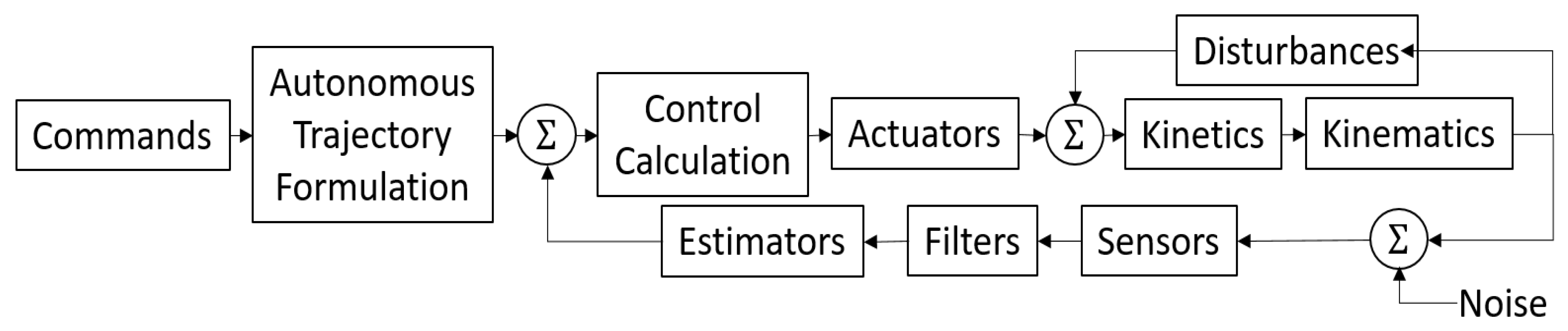
2.2. Autonomous Trajectory Generation

The goal is to have an intelligent system accept a desired endstate from the user and use that to autonomously created the entire maneuver trajectory without assistance. This maneuver trajectory will be used subsequently to formulate the deterministic self-awareness statement. One approach to autonomous trajectory generation is to impose a structure. Inspired by the nature of the exponential function as a solution-form for differential equations of motion, this structure will be imposed here.

The simple motion ordinary differential equation $\dot{z}=Az$ can be assumed to have an exponential solution. The solution for $z\left(t\right)$ may be differentiated and substituted back into the original motion equation to solve for the constants, $A$ and $\lambda .$ Additionally, recall that Euler’s Formula may be use to express the exponential as a sum of sines and cosines as seen in Equations (12) and (13), where the initial condition is assumed quiescent, eliminating the cosine:

$$z=A{e}^{\lambda t}\to \dot{z}=A\lambda e^{\lambda t}\to \ddot{z}=A{\lambda }^2{e}^{\lambda t}$$

(12)

If a nominal sine curve constitutes a position trajectory, and the first and second derivatives, respectively, constitute the velocity and acceleration trajectory per Equation (13):

$$z=Asin\left(\omega t\right)\to \dot{z}=A\omega cos\left(\omega t\right)\to \ddot{z}=-A{\omega }^{2}sin\left(\omega t\right)$$

(13)

A brief quiescent period $\mathrm{\Delta }{t}_{quiescant}$ (for trouble-shooting) is preferred, followed by a maneuver from the initial position (amplitude, $A_0$) to a commanded position (amplitude, $A$) in a specified maneuver time, $\mathrm{\Delta }{t}_{maneuver}$, subsequently followed by regulation at the new position, as depicted in Figure 3, where overshoot, oscillation, and settling are all undesirable traits. The following paragraph illustrates a systematic procedure to modify the nominal sine equation to achieve these desires while also ensuring smooth initiation of the maneuver (to avoid exciting un-modeled flexible vibration modes).

A nominal sine curve$z=Asin\left(\omega t\right)$ is depicted in Figure 3b represented by the thick-dashed line. Note that it starts abruptly at time$t=0$, while a smooth initiation is preferred to permit future expansion to flexible multi-body equations of motion (while rigid body dynamics are assumed here). The low point occurring at time $t=\frac{3T}{4}$ is desired to be placed at the designated maneuver time ($t=5$ here, assuming a five second quiescent period).

1.

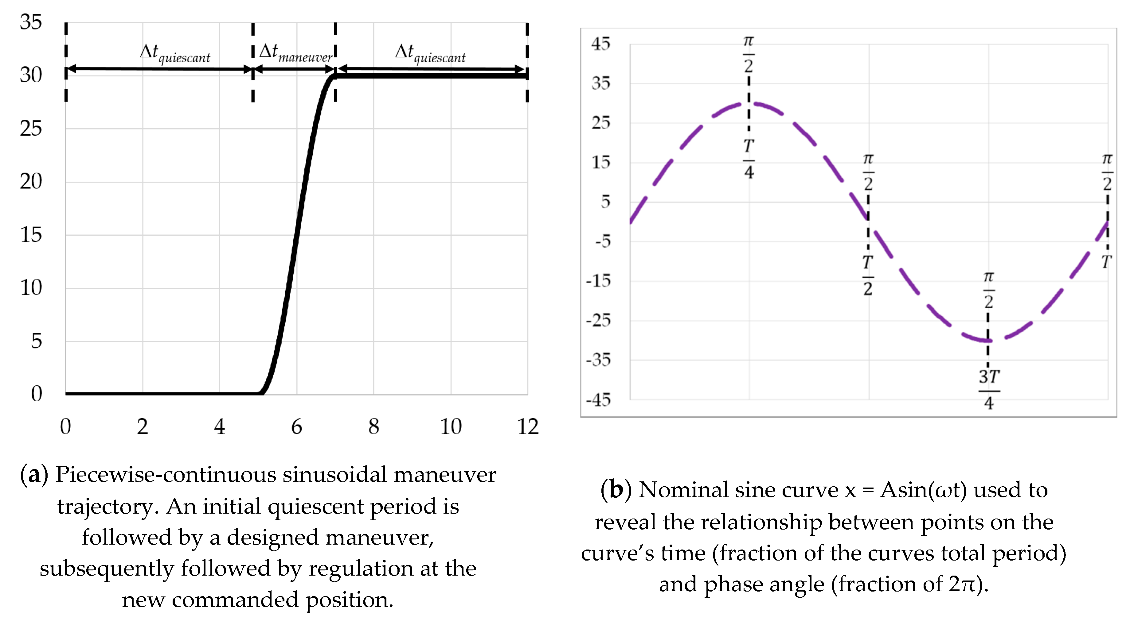
Choose the maneuver time: $\mathrm{\Delta }{t}_{maneuver}=2$ is used here illustratively. Express the maneuver time as a portion (half) of the total sinusoidal period, $T$, as depicted in Figure 3b.

-

The result is Equation (14):

$$\omega =\frac{2\pi }{T}\to \mathrm{\Delta }{t}_{maneuver}=\frac{\pi }{2}+\frac{\pi }{2}=\pi =\frac{T}{2}$$

(14)

Important side comment: Δtmaneuver is provided by the user, thus, this time period can be optimized (often represented as t*) to meet any number of cost functions, J and constraint equations.

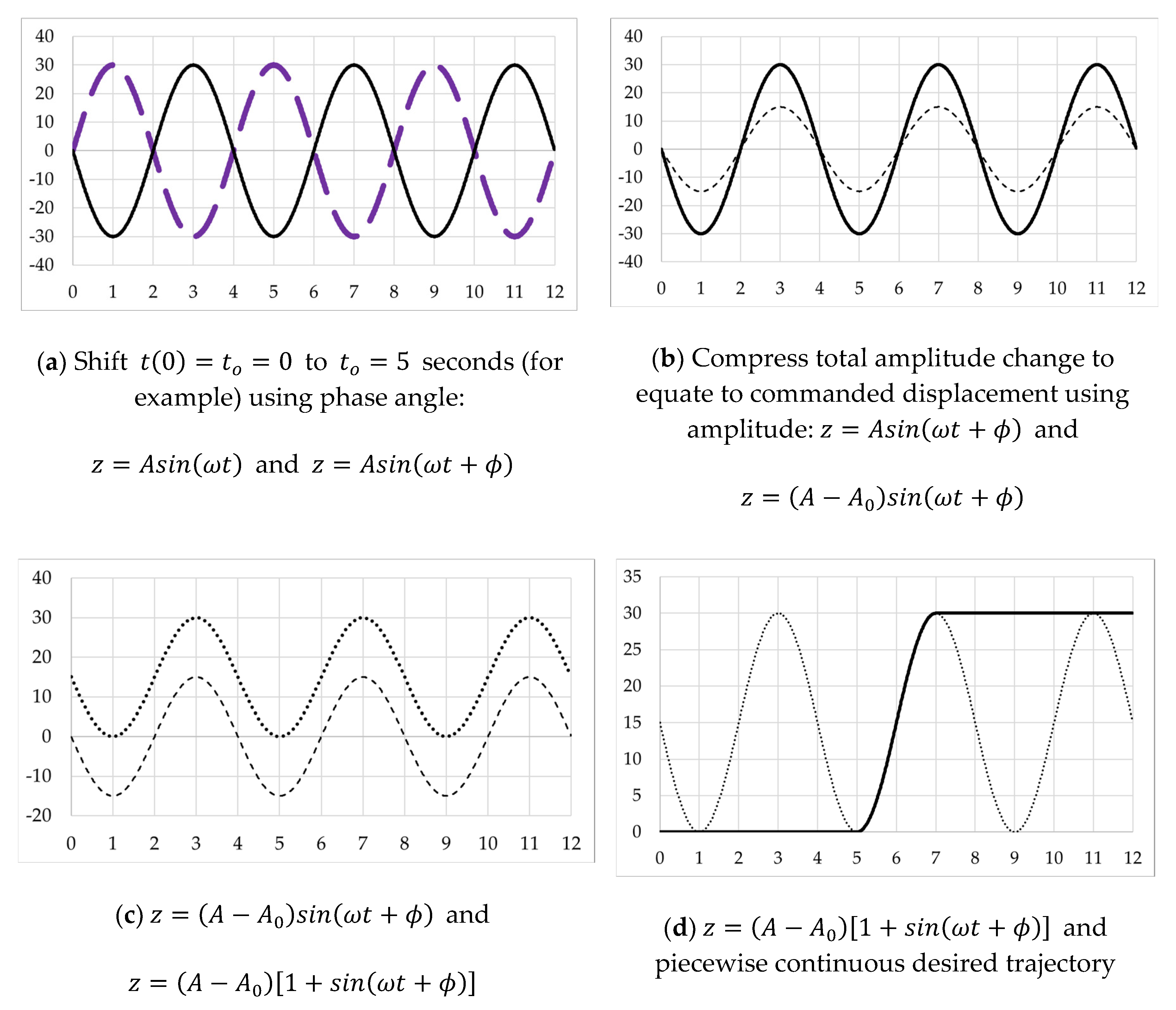
2.

Phase shift the curve to place the smooth low-point from $t=3$ to the desired maneuver start time, following the quiescent period at$t_{quiescant}=5$.

-

The result is Equation (15) plotted in Figure 4a:

$$z=Asin\left(\omega t\right)\to z=Asin\left(\omega t+\varphi \right)$$

(15)

3.

Compress the amplitude for the desired final change in amplitude to equate to the top-to-bottom total of curve.

-

The result is Equation (16) plotted in Figure 4b:

$$z=\left(A-A_0\right)sin\left(\omega t+\varphi \right)$$

(16)

4.

Amplitude-shift the curve up for smooth initiation at arbitrary starting position used here by adding$A_0$.

-

The result is Equation (17) plotted in Figure 4c:

$$z=\left(A-A_0\right)\left[1+sin\left(\omega t+\varphi \right)\right]$$

(17)

5.

Craft a piecewise continuous trajectory such that amplitude is zero until the termination of $t_{quiescant}$. Follow the sinusoidal trajectory during the maneuver time indicated by $\mathrm{\Delta }{t}_{maneuver}$, and then hold the final amplitude afterwards.

-

The result is Equation (18) plotted in Figure 4d:

$$for \{\begin{array}{c}t<t_{quiescant}\\ t_{quiescant}\le t<t_{quiescant}+\mathrm{\Delta }{t}_{maneuver}\\ t\ge t_{quiescant}+\mathrm{\Delta }{t}_{maneuver}\end{array}\to \begin{array}{c}z=A_0\\ z=\left(A-A_0\right)\left[1+sin\left(\omega t+\varphi \right)\right]\\ z=A\end{array}$$

(18)

6.

Differentiating Equation (17), derive the full state trajectory per Equations (19)–(21), establishing the second portion of the piecewise continuous trajectory in Equation (18) and Figure 4d, noting that Equation (19) exactly matches the second portion of Equation (18):

$$z_d=A_0+\frac{\left(A-A_0\right)}{2}\left[1+sin\left(\frac{\pi }{\mathrm{\Delta }{t}_{maneuver}}\left(t+\frac{3\mathrm{\Delta }{t}_{maneuver}}{2}-\mathrm{\Delta }{t}_{quiescant}\right)\right)\right]$$

(19)

$${\dot{z}}_d=\frac{\left(A-A_0\right)}{2}\left(\frac{\pi }{\mathrm{\Delta }{t}_{maneuver}}\right)cos\left(\frac{\pi }{\mathrm{\Delta }{t}_{maneuver}}\left(t+\frac{3\mathrm{\Delta }{t}_{maneuver}}{2}-\mathrm{\Delta }{t}_{quiescant}\right)\right)$$

(20)

$${\ddot{z}}_d=-\frac{\left(A-A_0\right)}{2}{\left(\frac{\pi }{\mathrm{\Delta }{t}_{maneuver}}\right)}^{2}sin\left(\frac{\pi }{\mathrm{\Delta }{t}_{maneuver}}\left(t+\frac{3\mathrm{\Delta }{t}_{maneuver}}{2}-\mathrm{\Delta }{t}_{quiescant}\right)\right)$$

(21)

$\mathrm{\Delta }{t}_{quiescant}$ is often omitted operationally, while $\mathrm{\Delta }{t}_{maneuver}$ is defined in Section 3 of this manuscript for any available control authority. Equations (19)–(21) are used to autonomously generate sway velocity and yaw rate trajectories for any initial and final state, any maneuver start time, and any desired total maneuver time (equivalently time at desired end state).

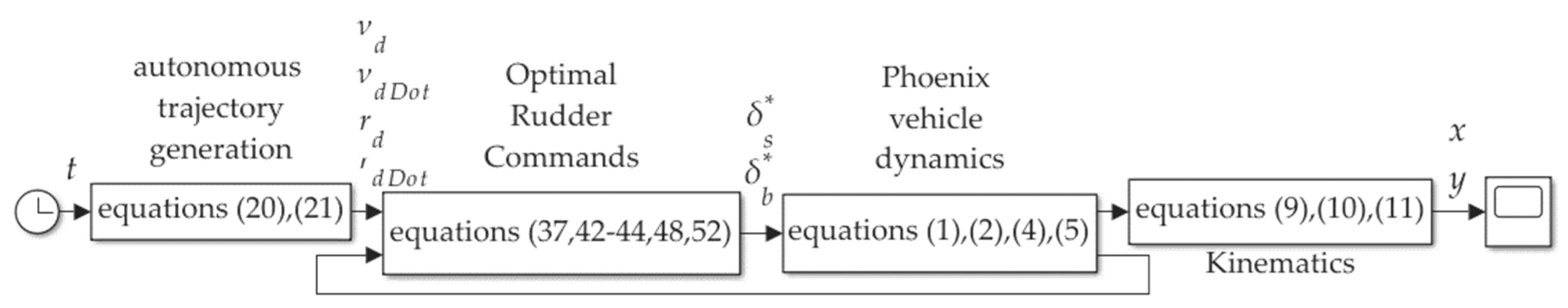
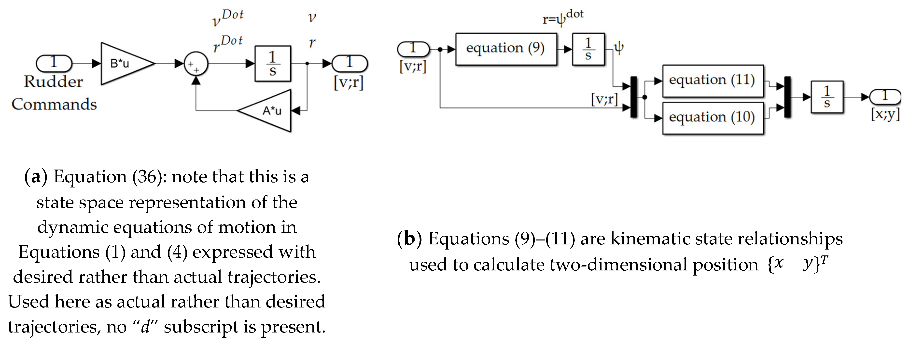
2.3. Topologies and Implementation in SIMULINK

Section 2.1 of this manuscript introduced the notion of asserting deterministic self-awareness statements invoking the mathematics of physics, and the description revealed the necessity of analytic expressions for trajectories that permit autonomous generation, and one such method is articulated in Section 2.2. Next, Section 2.3 displays topologies using the SIMULINK program where equation numbers were used as labels, and those equation numbers beg further explanation. Section 3 contains detailed development (from first principles) of the proposed method of deterministic artificial intelligence, and along the way, equations are labeled consistent with the presentations of topologies in Section 2. The first principles are the work of such famous scientists as Newton, Euler, and Chasle and some modern expressions are cited including Kane, Goldstein, Wie. The principles are presented as factually self-evident without much articulation, instead cited for independent pursuit by the reader.

3. Results

Stemming from the earlier described first principles [97,98,99,100,101,102,103,104,105,106,107,108], whose classical usage is described in [86,87,88,89,90,91,92,93,94,95,96], we accept these principles and adopt them as deterministic self-awareness statements. Next, we illustrate the parameterization of the statements in standard state-variable form [81,82,83,84,85]. We illustrate simple learning techniques that are honestly indistinguishable from non-linear adaptive control techniques [68,69,70,71,72,73] mentioned as “the lineage” of the subsequent technique presented: optimal learning using the state-variable formulation to highlight the pseudo-inverse optimal solution as the learning relationship. Nonlinear-adaptive techniques still require tuning, while the optimal learning relationship proposed here negates this requirement. The assertion of self-awareness statements is validated with several maneuvers, while the validating simulations with optimal learning are expressed in the presentation of the empirically derived relationship between maximum available actuation versus achievable minimum maneuver time (using both assertion of self-awareness statements and optimal learning). The motivation for this is presented at the end of the section: a nominal implementation procedure for deterministic artificial intelligence, whose first step is to establish minimum achievable maneuver time as a function of available actuators. The implementation methods bring Section 3 to a close, while Section 4 includes an operational implementation checklist.

3.1. Articulate Optimal Deterministic Self-Awareness Statement

Equations (22)–(25) articulate the equations of motion from Equations (7)–(9) expressed using desired trajectories indicated by subscript “d”. This comprises the first step of applying the deterministic artificial intelligence technique. Learning will be described in Section 3.3 and Section 3.4 after first reformulating the dynamics in Section 3.2.

$${\mathrm{₵}}_1{\dot{\nu }}_d+{\mathrm{₵}}_2{\dot{r}}_d+{\mathrm{₵}}_3{\nu }_d+{\mathrm{₵}}_4{r}_d\equiv {\mathrm{₵}}_{u_1}{\delta }_s$$

(22)

$${\mathrm{₵}}_5{\dot{\nu }}_d+{\mathrm{₵}}_6{\dot{r}}_d+{\mathrm{₵}}_7{\nu }_d+{\mathrm{₵}}_8{r}_d={\mathrm{₵}}_{u_2}{\delta }_s$$

(23)

$$\frac{{\mathrm{₵}}_1{\dot{\nu }}_d+{\mathrm{₵}}_2{\dot{r}}_d+{\mathrm{₵}}_3{\nu }_d+{\mathrm{₵}}_4{r}_d}{{\mathrm{₵}}_{u_1}}\equiv {\delta }_s$$

(24)

$$\frac{{\mathrm{₵}}_5{\dot{\nu }}_d+{\mathrm{₵}}_6{\dot{r}}_d+{\mathrm{₵}}_7{\nu }_d+{\mathrm{₵}}_8{r}_d}{{\mathrm{₵}}_{u_2}}={\delta }_s$$

(25)

Note: Equations (22) through (25) do not yet have learned estimates (which are indicated by superscript $\widehat{}$). These equations define the deterministic self-awareness statements to be asserted and subsequently learning will be applied to these statements as elaborated in Section 3.3 and Section 3.4. ${\mathrm{₵}}_i\forall i{{\displaystyle \cap }}^{}\left(1\dots 8\right)$ and ${\mathrm{₵}}_{u_1}\forall i{{\displaystyle \cap }}^{}\left(1\dots 2\right)$ defined in Equations (1)–(8) contain $m,I_z,m{x}_g$, and these values will be assumed known for use in Equations (22)–(25).

3.2. Formulate Optimal Deterministic Self-Awareness Statement in MIMO State Space Form

This section derives the full-form state-variable representation of the optimal deterministic self-awareness statement, where ${\delta }_s=-{\delta }_b$ rudder constraint equation is not enforced. Rudders are free to be designed separately in a “many-in, many-out” (MIMO) formulation. Isolate $\dot{\upsilon }$ in Equation (24), and then isolate $\dot{r}$ in Equation (25):

$${\dot{\nu }}_d=-\frac{{\mathrm{₵}}_2}{{\mathrm{₵}}_1}{\dot{r}}_d-\frac{{\mathrm{₵}}_3}{{\mathrm{₵}}_1}{\nu }_d-\frac{{\mathrm{₵}}_4}{{\mathrm{₵}}_1}{r}_d+\frac{{\mathrm{₵}}_{u_1}}{{\mathrm{₵}}_1}{\delta }_s$$

(26)

$${\dot{r}}_d=-\frac{{\mathrm{₵}}_5}{{\mathrm{₵}}_6}{\dot{\nu }}_d-\frac{{\mathrm{₵}}_7}{{\mathrm{₵}}_6}{\nu }_d-\frac{{\mathrm{₵}}_8}{{\mathrm{₵}}_6}{r}_d-\frac{{\mathrm{₵}}_{u_2}}{{\mathrm{₵}}_6}{\delta }_b$$

(27)

Isolate ${\dot{\upsilon }}_d$ by substituting Equation (27) into Equation (26):

$${\mathrm{₵}}_1{\dot{\nu }}_d+\frac{{\mathrm{₵}}_2}{{\mathrm{₵}}_6}\left(-{\mathrm{₵}}_5{\dot{\nu }}_d-{\mathrm{₵}}_7{\nu }_d-{\mathrm{₵}}_8{r}_d-{\mathrm{₵}}_{u_2}{\delta }_b\right)+{\mathrm{₵}}_3{\nu }_d+{\mathrm{₵}}_4{r}_d={\mathrm{₵}}_{u_1}{\delta }_s$$

(28)

$$\left({\mathrm{₵}}_1-\frac{{\mathrm{₵}}_2}{{\mathrm{₵}}_5{\mathrm{₵}}_6}\right){\dot{\nu }}_d+\left({\mathrm{₵}}_3-\frac{{\mathrm{₵}}_2}{{\mathrm{₵}}_6}{\mathrm{₵}}_7\right){\nu }_d+\left({\mathrm{₵}}_4-\frac{{\mathrm{₵}}_2}{{\mathrm{₵}}_6}{\mathrm{₵}}_8\right)r_d={\mathrm{₵}}_{u_1}{\delta }_s+\frac{{\mathrm{₵}}_2}{{\mathrm{₵}}_6}{\mathrm{₵}}_{u_2}{\delta }_b$$

(29)

$${\dot{\nu }}_d=\frac{1}{\left({\mathrm{₵}}_1-\frac{{\mathrm{₵}}_2}{{\mathrm{₵}}_5{\mathrm{₵}}_6}\right)}\left[-\left({\mathrm{₵}}_3-\frac{{\mathrm{₵}}_2}{{\mathrm{₵}}_6}{\mathrm{₵}}_7\right){\nu }_d-\left({\mathrm{₵}}_4-\frac{{\mathrm{₵}}_2}{{\mathrm{₵}}_6}{\mathrm{₵}}_8\right)r_d+{\mathrm{₵}}_{u_1}{\delta }_s+\frac{{\mathrm{₵}}_2}{{\mathrm{₵}}_6}{\mathrm{₵}}_{u_2}{\delta }_b\right]$$

(30)

$${\dot{\nu }}_d=\underset{a_1}{\underbrace{-\frac{{\mathrm{₵}}_3-\frac{{\mathrm{₵}}_2}{{\mathrm{₵}}_6}{\mathrm{₵}}_7}{{\mathrm{₵}}_1-\frac{{\mathrm{₵}}_2}{{\mathrm{₵}}_5{\mathrm{₵}}_6}}}}{\nu }_d-\underset{a_2}{\underbrace{\frac{{\mathrm{₵}}_4-\frac{{\mathrm{₵}}_2}{{\mathrm{₵}}_6}{\mathrm{₵}}_8}{{\mathrm{₵}}_1-\frac{{\mathrm{₵}}_2}{{\mathrm{₵}}_5{\mathrm{₵}}_6}}}}{r}_d+\underset{b_1}{\underbrace{\frac{{\mathrm{₵}}_{u_1}}{{\mathrm{₵}}_1-\frac{{\mathrm{₵}}_2}{{\mathrm{₵}}_5{\mathrm{₵}}_6}}}}{\delta }_s+\underset{b_2}{\underbrace{\frac{\frac{{\mathrm{₵}}_2}{{\mathrm{₵}}_6}{\mathrm{₵}}_{u_2}}{{\mathrm{₵}}_1-\frac{{\mathrm{₵}}_2}{{\mathrm{₵}}_5{\mathrm{₵}}_6}}}}{\delta }_b$$

(31)

$${\dot{\nu }}_d=a_1{\nu }_d-a_2{r}_d+b_1{\delta }_s+b_2{\delta }_b$$

(32)

Isolate $\dot{r}$ by substituting Equation (32) into Equation (27):

$${\dot{r}}_d=-\frac{{\mathrm{₵}}_5}{{\mathrm{₵}}_6}\left(a_1{\nu }_d+a_2{r}_d+b_1{\delta }_s+b_2{\delta }_b\right)-\frac{{\mathrm{₵}}_7}{{\mathrm{₵}}_6}{\nu }_d-\frac{{\mathrm{₵}}_8}{{\mathrm{₵}}_6}{r}_d-\frac{{\mathrm{₵}}_{u_2}}{{\mathrm{₵}}_6}{\delta }_b$$

(33)

$${\dot{r}}_d=\underset{a_3}{\underbrace{\left(-\frac{{\mathrm{₵}}_5}{{\mathrm{₵}}_6}{a}_1-\frac{{\mathrm{₵}}_7}{{\mathrm{₵}}_6}\right)}}{\nu }_d+\underset{a_4}{\underbrace{\left(-\frac{{\mathrm{₵}}_5}{{\mathrm{₵}}_6}{a}_{ }-\frac{{\mathrm{₵}}_8}{{\mathrm{₵}}_6}\right)}}{r}_d+\underset{b_1=b_3}{\underbrace{b_1}}{\delta }_s+\underset{b_4}{\underbrace{\left(b_2-\frac{{\mathrm{₵}}_{u_2}}{{\mathrm{₵}}_6}\right)}}{\delta }_b$$

(34)

$${\dot{r}}_d=a_3{\nu }_d+a_4{r}_d+b_3{\delta }_s+b_4{\delta }_b$$

(35)

Parameterize in a general form $\dot{x}=Ax$ to reveal optimal rudder commands based on the deterministic self-awareness statement:

$$\left\{\begin{array}{c}{\dot{\nu }}_d\\ {\dot{r}}_d\end{array}\right\}=\left[\begin{array}{cc}{a}_1& a_2\\ a_3& a_4\end{array}\right]\left\{\begin{array}{c}{\nu }_d\\ r_d\end{array}\right\}+\left[\begin{array}{cc}{b}_1& b_2\\ b_3& b_4\end{array}\right]\left\{\begin{array}{c}{\delta }_s\\ {\delta }_b\end{array}\right\}$$

(36)

$$\left\{\begin{array}{c}{\delta }_s^{*}\\ {\delta }_b^{*}\end{array}\right\}={\left[\begin{array}{cc}{b}_1& b_2\\ b_3& b_4\end{array}\right]}^{-1}\left(\left\{\begin{array}{c}{\dot{\nu }}_d\\ {\dot{r}}_d\end{array}\right\}-\left[\begin{array}{cc}{a}_1& a_2\\ a_3& a_4\end{array}\right]\left\{\begin{array}{c}{\nu }_d\\ r_d\end{array}\right\}\right)$$

(37)

Note: Equations (36) and (37) do not yet have learned estimates (which are indicated by a “hat” superscript $\widehat{}$). ${\mathrm{₵}}_i\forall i{{\displaystyle \cap }}^{}\left(1\dots 8\right)$ and ${\mathrm{₵}}_{u_1}\forall i{{\displaystyle \cap }}^{}\left(1\dots 2\right)$ defined in Equations (1)–(8) contain $m,I_z,m{x}_g$, and these values will be assumed known for use in Equations (36) and (37). These equations define the deterministic self-awareness statements to be asserted and subsequently learning will be applied to these statements as elaborated in Section 3.3 and Section 3.4.

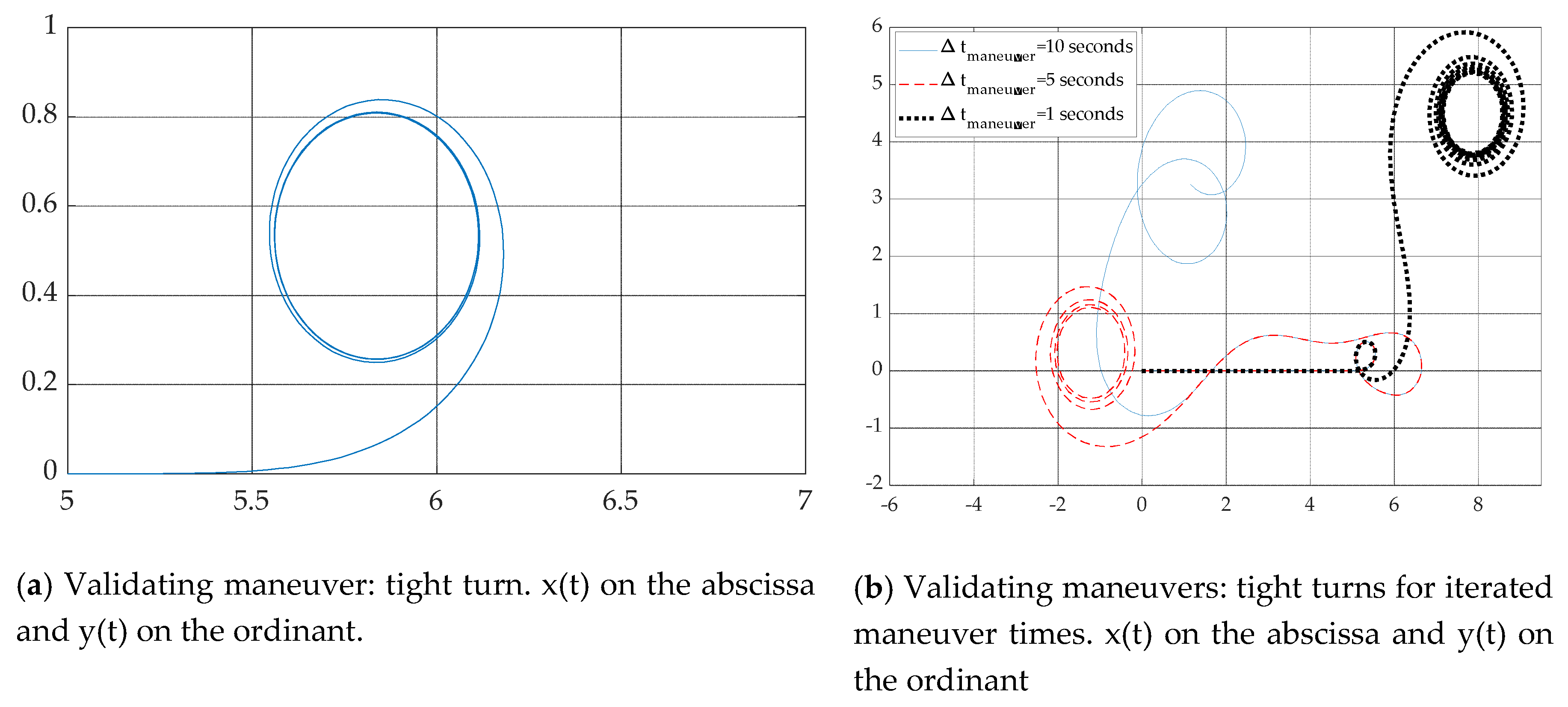
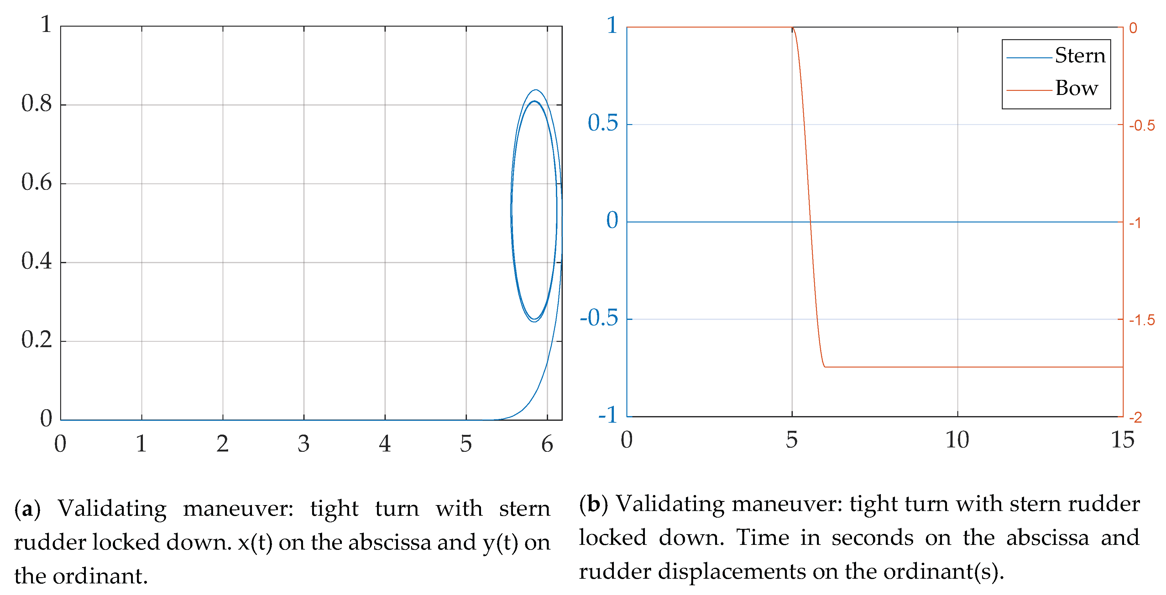
3.3. Validating Simulations

This section displays many simulations of various maneuvers and scenarios to validate a functioning simulation and the ability of the proposed method of deterministic artificial intelligence to control the unmanned underwater. Figure 5, Figure 6, Figure 7, Figure 8 and Figure 9 illustrate general topologies with inputs, mappings, and outputs. The mappings are labeled with equation numbers elaborated in Section 2 and Section 3 of this manuscript, permitting readers to create their own simulations using this manuscript as a guide. For operational implementation, the exact SIMULINK program may be used to command and control laboratory hardware by replacing the “Phoenix vehicle dynamics” block with electrical connectivity to the lab hardware.

Figure 5 displays the SIMULINK simulation of the equations developed in Section 3 of this manuscript, and was used to produce the validating simulations presented in Section 3. The simulation was also used to develop the coding procedure and operational implementation procedure presented in Section 4. These individual blocks displayed in Figure 5 are expanded in Figure 6, Figure 7, Figure 8 and Figure 9. Compare Figure 5 to Figure 2 to reveal assumptions of known or subsequently executable components: specific actuators, sensors, state observers, filters, and specific disturbances (withheld for future research seeking the limits of the robustness of the proposed techniques).

Figure 6 displays sub-systems of Figure 5, specifically the second subsystem from the left labeled “Optimal Rudder Commands.” The subsystem displayed in Figure 6 accepts the desired motion states and the actual motion states as inputs and outputs the two-norm optimal rudder commands using Equation (37), whose constants are learned by simple methods in Equations (42)–(44), or alternatively two-norm optimal learning in Equation (52) with Equation (48) and analytic expression used for solving the location of the center of gravity, which appears nonlinearly coupled with the vehicle mass.

Figure 7 displays the simulation blocks for simple learning which appears as the upper left block in Figure 6. Simple learning uses Equation (42) to learning the vehicle mass, which is used in Equation (43) to learn the time-varying location of the vehicle center of gravity, while Equation (44) is used to learn the mass moments of inertia.

Figure 9 displays the simulation of the kinematic motion state relationships expressed in Equations (9)–(11), and this figure finalizes the presentation of the SIMULINK program created for validating simulations.

Recall that no tuning was required and nonetheless motion states are controlled through several types of maneuvers in Figure 10 and Figure 11. Figure 11 also displays the nature of rudder motions where a single rudder is locked-down (either intentionally or by damage received while underway).

Following this brief demonstration of utility of self-awareness, the next section introduces two paradigms for learning: simple and optimal to allow self-awareness to learn a time-varying self-awareness. Following the technical developments of Section 3.3, the reader will have definitions for all the equations in the topology of Figure 5, Figure 6, Figure 7, Figure 8 and Figure 9 and will be in a position to attempt their own algorithm development. With that motivation, Section 3.5 of the manuscript will list a procedure to create software to control unmanned underwater vehicles, but then afterwards illustrate the use of the procedure. The self-awareness statement, together with optimal learning, will be shown to reveal the required actuator authority necessary to accomplish an unspecified maneuver duration.

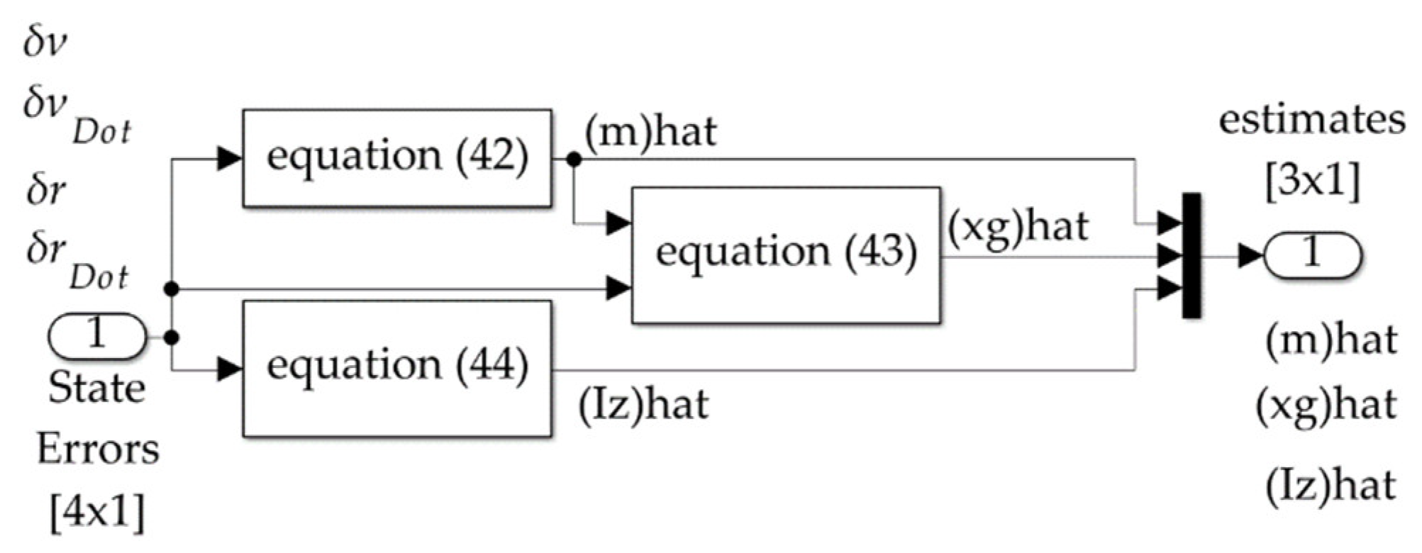
3.4. Deterministic Artificial Intelligence Simple-Learning

Start by defining variables and states $m,I_z,m{x}_g$. Then, rewrite the equations of motion isolating the states to be learned:

$$\left(m-Y_{\dot{\nu }}\right)\dot{\nu }-\left(Y_{\dot{r}}-m{x}_G\right)\dot{r}=Y_{\nu }\nu +\left(Y_r-m\right)r+Y_{{\delta }_s}{\delta }_s+Y_{{\delta }_b}{\delta }_b$$

(38)

$$\left(\dot{\nu }+r\right)m+\left(\dot{r}\right)m{x}_G=Y_{\dot{\nu }}\dot{\nu }+Y_{\dot{r}}\dot{r}+Y_{\upsilon }\upsilon +Y_{r}r+Y_{{\delta }_s}{\delta }_s+Y_{{\delta }_b}{\delta }_b$$

(39)

$$\left(m{x}_G-N_{\dot{\nu }}\right)\dot{\nu }-\left(N_{\dot{r}}-I_z\right)\dot{r}=N_{\nu }\nu +\left(N_r-m{x}_G\right)r+N_{{\delta }_s}{\delta }_s+N_{{\delta }_b}{\delta }_b$$

(40)

$$\left(0\right)m-\left(\dot{\nu }+r\right)m{x}_G+\left(\dot{r}\right)I_z=N_{\dot{\nu }}\dot{\nu }+N_{\dot{r}}\dot{r}+N_{\upsilon }\upsilon +N_{r}r+Y_{{\delta }_s}{\delta }_s+Y_{{\delta }_b}{\delta }_b$$

(41)

Use classical terms that are proportional to the error and error rate (derivative). The reader familiar with classical proportional, derivative (PD) control [80,81,82] will recognize the approach, but note that we are not formulating a feedback control signal using a PD controller; instead, we are learning the presumed unknown parameters in the deterministic self-awareness statement with proportional and derivative components, and then using that self-awareness statement to formulate the control. Let:

$$\widehat{m}=m_0-K_{m_1}\left({\dot{\nu }}_d-\dot{\nu }\right)-K_{m_1}\left({\nu }_d-\nu \right)$$

(42)

$$\widehat{m{x}_G}={\left(m{x}_G\right)}_0-K_{m{x}_G{}_1}\left(m{x}_G\right)\to {\widehat{x}}_G=\frac{{\widehat{mx}}_G}{\widehat{m}}$$

(43)

$${\widehat{I}}_Z={\widehat{I}}_Z{}_0-K_{I_1}\left({\dot{r}}_d-\dot{r}\right)-K_{I_2}\left(r_d-r\right)$$

(44)

It is presumed here that any/all states are knowable by using sensors, inertial navigation, simultaneous location and mapping (SLAM), state observers, Kalman filters, and such. Thus, in Figure 5, full state knowledge is assumed in the feedback signal used for learning.

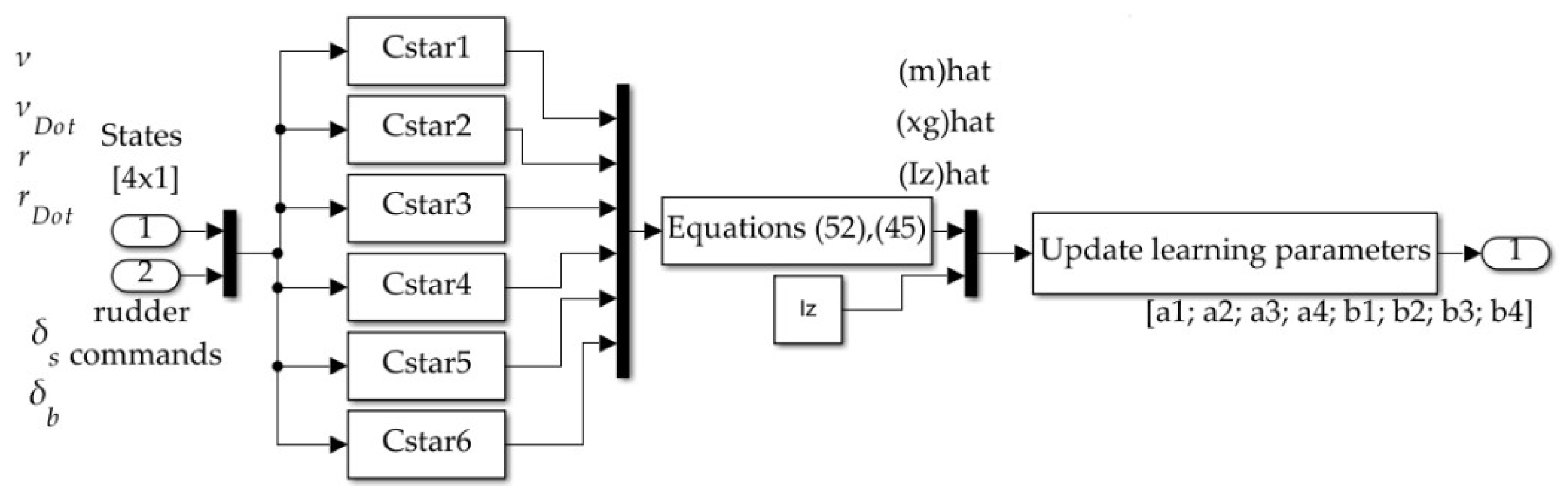
3.5. Deterministic Artificial Intelligence Optimal Learning

Recall from Equations (2) and (5) the constants starting with ${\mathrm{₵}}_i\forall i=1,2,\dots 8,$ ending with $a_i\forall i=1,2,3,4$ and $b_i\forall i=1,2,3,4$ require knowledge of mass, $\widehat{m}$ and mass moment of inertia, ${\widehat{I}}_Z$. Section 3.3 describes a simple learning approach to discover values of $\widehat{m}$ and ${\widehat{I}}_Z$. This section seeks to express an optimal learning methodology, eliminating the need for tuning. Solve Equations (1) and (4) for the product $m{x}_G$. Solving Equation (1) for the product of mass and location of the center of gravity, $m{x}_G$ produces Equation (45):

$$m{x}_G=\frac{1}{\dot{r}}\left[Y_{\dot{\nu }}\dot{\nu }+Y_{\dot{r}}\dot{r}+Y_{\upsilon }\upsilon +Y_{r}r+Y_{{\delta }_s}{\delta }_s+Y_{{\delta }_b}{\delta }_b-m\left(\dot{\nu }+r\right)\right]$$

(45)

then substitute the result of Equation (45) into Equation (4) to produce Equation (46), a new version of the second equation of the deterministic self-awareness statement, which may be formulated to parameterize with $m$ and $I_z$ as the states resulting in Equation (46):

$$\begin{gathered} \left(\dot{\nu }+\dot{r}\right)\left[\frac{1}{\dot{r}}\left(Y_{\dot{\nu }}\dot{\nu }+Y_{\dot{r}}\dot{r}+Y_{\upsilon }\upsilon +Y_{r}r+Y_{{\delta }_s}{\delta }_s+Y_{{\delta }_b}{\delta }_b-m\left(\dot{\nu }+r\right)\right)\right]+\dot{r}{I}_z \\ =N_{\dot{\nu }}\dot{\nu }+N_{\dot{r}}\dot{r}+N_{\nu }\nu +N_{r}r+N_{{\delta }_s}{\delta }_s+N_{{\delta }_b}{\delta }_b \end{gathered}$$

(46)

$$\begin{array}{cc}\hfill \underset{{\mathrm{₵}}_1^{*}}{\underbrace{\left(\frac{\dot{\nu }+\dot{r}}{\dot{r}}\dot{\nu }\right)}}m-\underset{{\mathrm{₵}}_2^{*}}{\underbrace{\dot{r}}}& I_z\hfill \\ & =\left(\dot{\nu }+\dot{r}\right)\left[\frac{1}{\dot{r}}\left(Y_{\dot{\nu }}\dot{\nu }+Y_{\dot{r}}\dot{r}+Y_{\upsilon }\upsilon +Y_{r}r+Y_{{\delta }_s}{\delta }_s+Y_{{\delta }_b}{\delta }_b-mr\right)\right]-N_{\dot{\nu }}\dot{\nu }-N_{\dot{r}}\dot{r}-N_{\nu }\nu \hfill \\ & -N_{r}r-N_{{\delta }_s}{\delta }_s-N_{{\delta }_b}{\delta }_b={\mathrm{₵}}_3^{*}\hfill \end{array}$$

(47)

Solve Equation (4) for the product of mass and location of the center of gravity, $m{x}_G:$

$$m{x}_G=\left(\frac{1}{\dot{\nu }+\dot{r}}\right)\left[-\dot{r}{I}_z+N_{\dot{\nu }}\dot{\nu }+N_{\dot{r}}\dot{r}+N_{\upsilon }\upsilon +N_{r}r+N_{{\delta }_s}{\delta }_s+N_{{\delta }_b}{\delta }_b\right]$$

(48)

then substitute the result of Equation (48) into Equation (1) to produce Equation (49), a new version of the first equation of the deterministic self-awareness statement, which may be formulated to parameterize with $m$ and $I_z$ as the states:

$$\begin{gathered} \left(\dot{\nu }+\dot{r}\right)m+\left(\frac{\dot{r}}{\nu +r}\right)\left[-\dot{r}{I}_z+N_{\dot{\nu }}\dot{\nu }+N_{\dot{r}}\dot{r}+N_{\upsilon }\upsilon +N_{r}r+N_{{\delta }_s}{\delta }_s+N_{{\delta }_b}{\delta }_b\right] \\ =Y_{\dot{\nu }}\dot{\nu }+Y_{\dot{r}}\dot{r}+Y_{\upsilon }\upsilon +Y_{r}r+Y_{{\delta }_s}{\delta }_s+Y_{{\delta }_b}{\delta }_b \end{gathered}$$

(49)

$$\begin{array}{cc}\hfill \underset{{\mathrm{₵}}_4^{*}}{\underbrace{\left(\dot{\nu }+\dot{r}\right)}}m\underset{{\mathrm{₵}}_5^{*}}{\underbrace{-\left(\frac{\dot{r}}{\nu +r}\right)}}& I_z\hfill \\ & =\left(\frac{\dot{r}}{\nu +r}\right)\left[N_{\dot{\nu }}\dot{\nu }+N_{\dot{r}}\dot{r}+N_{\upsilon }\upsilon +N_{r}r+N_{{\delta }_s}{\delta }_s+N_{{\delta }_b}{\delta }_b\right]+Y_{\dot{\nu }}\dot{\nu }+Y_{\dot{r}}\dot{r}+Y_{\upsilon }\upsilon \hfill \\ & +Y_{r}r+Y_{{\delta }_s}{\delta }_s+Y_{{\delta }_b}{\delta }_b={\mathrm{₵}}_6^{*}\hfill \end{array}$$

(50)

Expressing Equations (47) and (50) together in state-variable form (i.e., “state space”) yields Equation (51), which may be inverted to solve for the optimal learned values for mass and mass moment of inertia in Equation (52), where the arbitrarily labeled constants are calculated in Equations (47) and (50) using desired states:

$$\left[\begin{array}{cc}{\mathrm{₵}}_1^{*}& {\mathrm{₵}}_2^{*}\\ {\mathrm{₵}}_4^{*}& {\mathrm{₵}}_5^{*}\end{array}\right]\left\{\begin{array}{c}m\\ I_z\end{array}\right\}=\left\{\begin{array}{c}{\mathrm{₵}}_3^{*}\\ {\mathrm{₵}}_6^{*}\end{array}\right\}$$

(51)

$$\left\{\begin{array}{c}\widehat{m}\\ {\widehat{I}}_z\end{array}\right\}={\left[\begin{array}{cc}{\mathrm{₵}}_1^{*}& {\mathrm{₵}}_2^{*}\\ {\mathrm{₵}}_4^{*}& {\mathrm{₵}}_5^{*}\end{array}\right]}^{-1}\left\{\begin{array}{c}{\mathrm{₵}}_3^{*}\\ {\mathrm{₵}}_6^{*}\end{array}\right\}$$

(52)

The location of the center of gravity may then be located by solving Equation (45) with all components known, except $x_G$. This estimate of the location of the center of gravity may then be located by solving Equation (45) with all components known, except $x_G$ together with Equation (52) provide the optimal learned values that should replace $m$, $x_G$ and $I_z$ in the deterministic self-awareness statements embodied in Equation (37) optimal rudder commands based on self-awareness, requiring updated intermediate constants $a_i\prime s$ and $b_i\prime s$ defined in Equations (31) and (34) necessitating updated intermediate constants ${\mathrm{₵}}_i\forall i{{\displaystyle \cap }}^{}\left(1\dots 8\right)$ and ${\mathrm{₵}}_{u_1}\forall i{{\displaystyle \cap }}^{}\left(1\dots 2\right)$ in Equations (2) and (5).

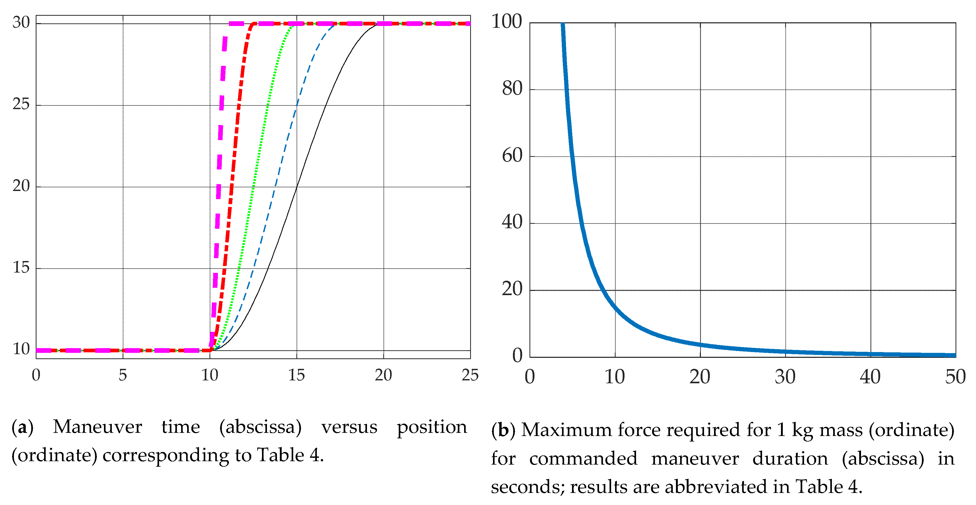
3.6. Optimize maneuver Time for the Allowable Maximum Non-Dimensional Force for a Representative Maneuver

One approach to designing maximum-performance maneuvers is to design the command to fit the amount of available control force (illustrated in

Table 4. Maneuvers and required maximum force corresponding to Figure 12a.

Maneuver Time	Max Force	Corresponding Line Font in Figure 4a
10	14.8	Thin, black solid
7.5	26.3	Thin, blue, dashed
5	59.2	Thin, green, dotted
2.5	236.8	Thick, red, dash-dot
1	1480.4	Thick, pink, dashed

Abbreviated results from Figure 12b.

corresponding to Figure 12a). Iterating maneuver times yield performance curves (Figure 12a), allowing engineers to understand how quickly a maneuver can be demanded, while Figure 12b reveals the force required to accomplish the maneuver depicted in Figure 12a, among others. These two key figures produce a design procedure where the available rudder force yields the minimum time maneuver that can be produced by that vehicle configuration. The resulting maneuver duration may be substituted into Equations (19)–(21) in place of $\mathrm{\Delta }{t}_{maneuver}$, producing full-state autonomously generated trajectories. Especially since deterministic artificial intelligence (in its error-optimal learning instantiation) requires no tuning, this single decision is the only thing required to formulate all other constituent analytic relationships elaborated in this manuscript.

3.7. Procedures to Implement Deterministic Artificial Intelligence as Proposed

Section 3.5 revealed an operational implementation procedure with the revelations of Figure 11a,b. This section succinctly describes a nominal procedure for use by operators of unmanned underwater vehicles to wish to apply the proposed deterministic artificial intelligence methods.

1. Choose hardware including actuators with identifiable maximal force output 2. Use maximal force output to select minimal maneuver time using Figure 12b 3. Use minimal maneuver time as $\mathrm{\Delta }{\mathrm{t}}_{\mathrm{maneuver}}$ in Equations (19)–(21) to autonomously produce full state “desired trajectories” 4. Use trajectories to formulate deterministic self-awareness statements 5. Implement learning method of choice

4. Discussion

The first three sections of this manuscript developed a proposed approach of deterministic artificial intelligence to control the motion of unmanned underwater vehicles. Section 4 discusses operational implementation. It is assumed the reader will have access to some kind of actuators, and the specific actuator is assumed to be (at this time) unknown. Thus, actuator selection is the first step of the implementation process. After the reader knows the control authority provided by their actuator selection, Section 4.1 gives the operational implementation procedure to implement the proposed methodology. The reader will notice the complete lack of tuning or other mathematical develop required after selection of the actuator is made.

4.1. Deterministic Artificial Intelligence Procedure

Assert deterministic self-awareness statement: Use Equations (22) and (23) with an initial assumed value of mass and mass moment of inertia to command the vehicle’s two rudders using Equation (37) optimally embodying Equations (24) and (25) versions of Equations (22) and (23)’s self-awareness statements.

1.

Use simple learning (Equations (42)–(44)) or optimal learning (Equation (52) with Equation (45)) to update the values of mass and mass moment of inertia, where in the instance of optimal learning the location of the center of gravity is provided by Equation (35). The update begins with substituting the values of the learned parameters into the values of the constants ${\mathrm{₵}}_i\forall i=1\dots 6$ (defined in Equation (2) and Equation (5)), leading to the values of constants $a_i,b_i\forall i=1\dots 4$ (defined in Equation (31) and Equation (34)) used in Equation (37) that command to both rudders.

a.

Replace $m$, $x_G$, and $I_z$ in the deterministic self-awareness statements intermediate constants ${\mathrm{₵}}_i\forall i{{\displaystyle \cap }}^{}\left(1\dots 8\right)$ and ${\mathrm{₵}}_{u_1}\forall i{{\displaystyle \cap }}^{}\left(1\dots 2\right)$ in Equations (2) and (5).

b.

Use intermediate constants ${\mathrm{₵}}_i\forall i{{\displaystyle \cap }}^{}\left(1\dots 8\right)$ and ${\mathrm{₵}}_{u_1}\forall i{{\displaystyle \cap }}^{}\left(1\dots 2\right)$ to find updated intermediate constants $a_i\prime s$ and $b_i\prime s$ defined in Equations (31) and (34)

c.

Use updated intermediate constants $a_i\prime s$ and $b_i\prime s$ in the optimal rudder commands of Equation (37), which include deterministic artificial intelligence self-awareness statements (thus, we are learning the vehicle’s self).

4.2. Operational Implementation Procedure

1.

Choose $\mathrm{\Delta }{t}_{maneuver}$ for the available control authority (by choice of actuators) from Figure 12b.

2.

Use Equations (19)–(21) to autonomously articulate a trajectory (state, velocity, and acceleration) that starts at the initial point and ends at the commanded point using $\mathrm{\Delta }{t}_{maneuver}$ from step 1.

3.

Use Equation (37) for optimal rudder commands developed using the deterministic self-awareness statement of rigid body motion, where constants are defined in (31) and (34) with constituent constants defined in Equations (2) and (5).

4.

Use Equations (42)–(44) for simple learning or Equation (52) with Equation (45) for optimal learning of time-varying, unknowable parameters $m,x_G, I_z$.

5.

Use the parameters learned in step 4 to update the constants and constituent constants, repeating step 3 optimal rudder commands

4.3. Follow-On Research

This manuscript described the development of the proposed techniques from first principles, articulated optimality, and illustrated step-by-step procedures for algorithm development and operational implementation. Future research includes critical analysis intended to reveal limitations of the technique. Algorithm discretization time step will be iterated to reveal the potential existence of a minimum processor speed required to run the algorithm. Simulated damage will be imposed on the vehicle to ascertain the efficacy of the method’s robustness. Parameter variation will be imposed to investigate the algorithms sensitivity and bridge to real-world implementation in lab and open ocean experiments. Disturbances (e.g., currents and wave action) will be added to reveal the method’s dynamic stiffness. It is noteworthy that any instance of disturbance where a physics-based mathematical description is available, those descriptions can be used to formulate deterministic self-awareness statements to augment those already presented in this manuscript. In essence, the vehicle can become aware of its disturbance environment as part of its self-awareness. The rigid body can know that it is an unmanned underwater vehicle in a specifically disturbed environment. Consideration will be given in future research to a reverse design procedure that permits the algorithm to tell the operator which actuator to purchase and install to accomplish some known maneuver driven by a trajectory tracking task given weigh-point guidance (not addressed here). An additional interesting procedure includes underactuated maneuvers that are nonetheless demanded by operational imperatives.

Lastly, experimentation should include comparison to existing solutions, particularly those described in the introduction of this manuscript (i.e., typical stochastic A.I. methods and other analytic methods articulated in Section 1). Experimentation is contingent upon further research funding.

References

- McCorduck, P.; Cfe, C. Machines Who Think: A Personal Inquiry into the History and Prospects of Artificial Intelligence, 2nd ed.; A.K. Peters, Ltd.: Matick, MA, USA, 2004; ISBN 1-56881-205-1. [Google Scholar]
- Russell, S.; Norvig, P. Artificial Intelligence: A Modern Approach, 2nd ed.; Prentice Hall: Upper Saddle River, NJ, USA, 2003; ISBN 0-13-790395-2. [Google Scholar]
- Berlinski, D. The Advent of the Algorithm. Harcourt Books; Harcourt: San Diego, CA, USA, 2000; ISBN 978-0-15-601391-8. [Google Scholar]
- Turing, A. Machine Intelligence. In The Essential Turing: The Ideas That Gave Birth to the Computer Age; Copeland, B.J., Ed.; Oxford University Press: Oxford, UK, 1948; p. 412. ISBN 978-0-19-825080-7. [Google Scholar]
- Russell, S.; Norvig, P. Artificial Intelligence: A Modern Approach, 3rd ed.; Prentice Hall: Upper Saddle River, NJ, USA, 2009; ISBN 978-0-13-604259-4. [Google Scholar]
- Dartmouth Summer Research Project on Artificial; Dartmouth College: Hanover, NH, USA, 1956.
- Schaeffer, J. Didn’t Samuel Solve That Game? In One Jump Ahead; Springer: Boston, MA, USA, 2009. [Google Scholar]
- Samuel, A.L. Some Studies in Machine Learning Using the Game of Checkers. IBM J. Res. Dev. 1959, 3, 210–229. [Google Scholar] [CrossRef]
- Crevier, D. AI: The Tumultuous Search for Artificial Intelligence; BasicBooks: New York, NY, USA, 1993; ISBN 0-465-02997-3. [Google Scholar]
- Howe, J. Artificial Intelligence at Edinburgh University: A Perspective; Informatics Forum: Edinburgh, UK, 2007. [Google Scholar]
- Simon, H.A. The Shape of Automation for Men and Management; Harper & Row: New York, NY, USA, 1965. [Google Scholar]
- Minsky, M. Computation: Finite and Infinite Machines; Prentice-Hall: Englewood Cliffs, NJ, USA, 1967; ISBN 978-0-13-165449-5. [Google Scholar]
- McCarthy, J. Artificial Intelligence: A paper symposium. In Artificial Intelligence: A General Survey; Lighthill, J., Ed.; Science Research Council: Newcastle, UK, 1973. [Google Scholar]
- ACM Computing Classification System: Artificial Intelligence; ACM: New York, NY, USA, 1998.
- Nilsson, N. Artificial Intelligence: A New Synthesis; Morgan Kaufmann: Burlington, VT, USA, 1998; ISBN 978-1-55860-467-4. [Google Scholar]
- Newquist, H. The Brain Makers: Genius, Ego, and Greed in the Quest for Machines That Think; Macmillan/SAMS: New York, NY, USA, 1994; ISBN 978-0-672-30412-5. [Google Scholar]
- NRC (United States National Research Council). Developments in Artificial Intelligence. In Funding a Revolution: Government Support for Computing Research; National Academy Press: Washington, DC, USA, 1999. [Google Scholar]
- Luger, G.F.; Stubblefield, W. Artificial Intelligence: Structures and Strategies for Complex Problem Solving, 5th ed.; Benjamin/Cummings: San Francisco, CA, USA, 2004; ISBN 978-0-8053-4780-7. [Google Scholar]
- Kurzweil, R. The Singularity Is Near; Penguin Books: London, UK, 2005; ISBN 978-0-670-03384-3. [Google Scholar]
- Markoff, J. Computer Wins on ‘Jeopardy!’: Trivial, It’s Not; The New York Times: New York, NY, USA, 2011. [Google Scholar]
- Ask the AI Experts: What’s Driving Today’s Progress in AI? McKinsey & Company: Brussels, Belgium, 2018.
- Kinect’s AI Breakthrough Explained. Available online: https://www.i-programmer.info/news/105-artificial-intelligence/2176-kinects-ai-breakthrough-explained.html (accessed on 29 July 2020).
- Rowinski, D. Virtual Personal Assistants & The Future Of Your Smartphone [Infographic]. Available online: https://readwrite.com/2013/01/15/virtual-personal-assistants-the-future-of-your-smartphone-infographic/ (accessed on 29 July 2020).
- AlphaGo—Google DeepMind. Available online: https://deepmind.com/research/case-studies/alphago-the-story-so-far (accessed on 29 July 2020).
- Artificial intelligence: Google’s AlphaGo beats Go master Lee Se-dol. BBC News. 12 March 2016. Available online: https://www.bbc.com/news/technology-35785875 (accessed on 10 June 2020).
- Metz, C. After Win in China, AlphaGo’s Designers Explore New AI after Winning Big in China. Available online: https://www.wired.com/2017/05/win-china-alphagos-designers-explore-new-ai/ (accessed on 29 July 2020).
- World’s Go Player Ratings. Available online: https://www.goratings.org/en/ (accessed on 29 July 2020).
- Kē Jié Yíng Celebrates His 19th Birthday, Ranking First in the World for Two Years. 2017. Available online: http://sports.sina.com.cn/go/2016-08-02/doc-ifxunyya3020238.shtml (accessed on 10 June 2020). (In Chinese).
- Clark, J. Why 2015 Was a Breakthrough Year in Artificial Intelligence. Bloomberg News. 8 December 2016. Available online: https://www.bloomberg.com/news/articles/2015-12-08/why-2015-was-a-breakthrough-year-in-artificial-intelligence (accessed on 10 June 2020).
- Reshaping Business with Artificial Intelligence. MIT Sloan Management Review. Available online: https://sloanreview.mit.edu/projects/reshaping-business-with-artificial-intelligence/ (accessed on 10 June 2020).
- Lorica, B. The State of AI Adoption. O’Reilly Media. 18 December 2017. Available online: https://www.oreilly.com/radar/the-state-of-ai-adoption/ (accessed on 10 June 2020).
- Allen, G. Understanding China’s AI Strategy. Center for a New American Security. 6 February 2019. Available online: https://www.cnas.org/publications/reports/understanding-chinas-ai-strategy (accessed on 10 June 2020).
- Review|How Two AI Superpowers—The U.S. and China—Battle for Supremacy in the Field. Washington Post, 2 November 2018.
- Alistair, D. Artificial Intelligence: You Know It Isn’t Real, Yeah? 2019. Available online: https://www.theregister.com/2019/02/22/artificial_intelligence_you_know_it_isnt_real_yeah (accessed on 10 June 2020).
- Stop Calling It Artificial Intelligence. Available online: https://joshworth.com/stop-calling-in-artificial-intelligence/ (accessed on 10 April 2020).
- AI Isn’t Taking over the World—It Doesn’t Exist yet. Available online: https://www.gbgplc.com/inside/ai/ (accessed on 10 April 2020).
- Poole, D.; Mackworth, A.; Goebel, R. Computational Intelligence: A Logical Approach; Oxford Press: New York, NY, USA, 1998. [Google Scholar]
- Legg, S.; Hutter, M. A Collection of Definitions of Intelligence. Front. Artif. Intell. Appl. 2007, 157, 17–24. [Google Scholar]
- Domingos, P. The Master Algorithm: How the Quest for the Ultimate Learning Machine Will Remake Our World; Basic Books: New York, NY, USA, 2015; ISBN 978-0-465-06192-1. [Google Scholar]
- Lindenbaum, M.; Markovitch, S.; Rusakov, D. Selective sampling for nearest neighbor classifiers. Mach. Learn. 2004, 54, 125–152. [Google Scholar] [CrossRef]
- Brutzman, D. A Virtual World for an Autonomous Underwater Vehicle. Ph.D. Thesis, Naval Postgraduate School, Monterey, CA, USA, 1994. Available online: https://calhoun.nps.edu/handle/10945/30801 (accessed on 21 April 2020).
- Sands, T.; Bollino, K.; Kaminer, I.; Healey, A. Autonomous Minimum Safe Distance Maintenance from Submersed Obstacles in Ocean Currents. J. Mar. Sci. Eng. 2018, 6, 98. [Google Scholar] [CrossRef] [Green Version]
- Deterministic Artificial Intelligence for Surmounting Battle Damage. FY19 Funded Research Proposal. Available online: https://calhoun.nps.edu/handle/10945/62087 (accessed on 20 April 2020).
- Sands, T.; Kim, J.; Agrawal, B. 2H Singularity-Free Momentum Generation with Non-Redundant Single Gimbaled Control Moment Gyroscopes. In Proceedings of the 45th IEEE Conference on Decision & Control, San Diego, CA, USA, 13–15 December 2006. [Google Scholar]
- Sands, T.; Kim, J.; Agrawal, B. Control Moment Gyroscope Singularity Reduction via Decoupled Control. In Proceedings of the IEEE SEC, Atlanta, GA, USA, 5–8 March 2009. [Google Scholar]
- Sands, T.; Kim, J.; Agrawal, B. Experiments in Control of Rotational Mechanics. Int. J. Autom. Contr. Int. Syst. 2016, 2, 9–22. [Google Scholar]
- Agrawal, B.; Kim, J.; Sands, T. Method and Apparatus for Singularity Avoidance for Control Moment Gyroscope (CMG) Systems without Using Null Motion. U.S. Patent Application No. 9567112 B1, 14 February 2017. [Google Scholar]
- Sands, T.; Lu, D.; Chu, J.; Cheng, B. Developments in Angular Momentum Exchange. Int. J. Aerosp. Sci. 2018, 6, 1–7. [Google Scholar] [CrossRef]
- Sands, T.; Kim, J.J.; Agrawal, B. Singularity Penetration with Unit Delay (SPUD). Mathematics 2018, 6, 23. [Google Scholar] [CrossRef] [Green Version]
- Lewis, Z.; Ten Eyck, J.; Baker, K.; Culton, E.; Lang, J.; Sands, T. Non-symmetric gyroscope skewed pyramids. Aerospace 2019, 6, 98. [Google Scholar] [CrossRef] [Green Version]
- Baker, K.; Culton, E.; Ten Eyck, J.; Lewis, Z.; Sands, T. Contradictory Postulates of Singularity. Mech. Eng. Res. 2020, 9, 28–35. [Google Scholar] [CrossRef] [Green Version]
- Wikipedia, Deterministic Algorithm. Available online: https://en.wikipedia.org/wiki/Deterministic_algorithm#:~:text=In%20computer%20science%2C%20a%20deterministic,the%20same%20sequence%20of%20states (accessed on 10 June 2020).
- Quora.com. Available online: https://www.quora.com/What-s-the-difference-between-a-deterministic-environment-and-a-stochastic-environment-in-AI (accessed on 10 June 2020).
- Baker, K.; Cooper, M.; Heidlauf, P.; Sands, T. Autonomous trajectory generation for deterministic artificial intelligence. Electr. Electron. Eng. 2019, 8, 59. [Google Scholar]
- Lobo, K.; Lang, J.; Starks, A.; Sands, T. Analysis of deterministic artificial intelligence for inertia modifications and orbital disturbances. Int. J. Control Sci. Eng. 2018, 8, 53–62. [Google Scholar] [CrossRef]
- Sands, T. Physics-based control methods. In Advances in Spacecraft Systems and Orbit Determination; Ghadawala, R., Ed.; InTechOpen: Rijeka, Croatia, 2012; pp. 29–54. [Google Scholar]
- Sands, T.; Lorenz, R. Physics-Based Automated Control of Spacecraft. In Proceedings of the AIAA SPACE, Pasadena, CA, USA, 14–17 September 2009; American Institute of Aeronautics and Astronautics: Reston, VA, USA, 2012. [Google Scholar]
- Sands, T. Improved magnetic levitation via online disturbance decoupling. Phys. J. 2015, 1, 272. [Google Scholar]
- National Air and Space Administration. Design of Low Complexity Model Reference Adaptive Controllers; Dryden: Fort Worth, TX, USA; California and Ames: Mountain View, CA, USA, 2012; ISBN 978-1793957245.
- Nguyen, N. Model-Reference Adaptive Control: A Primer; Springer: New York, NY, USA, 2019; ISBN 978-3319563923. [Google Scholar]
- National Air and Space Administration. Complexity and Pilot Workload Metrics for the Evaluation of Adaptive Flight Controls on a Full Scale Piloted Aircraft; Dryden: Fort Worth, TX, USA; California and Ames: Mountain View, CA, USA, 2019; ISBN 978-1794408159.
- Sands, T. Space systems identification algorithms. J. Space Exp. 2017, 6, 138–149. [Google Scholar]
- Sands, T.; Kenny, T. Experimental piezoelectric system identification. J. Mech. Eng. Autom. 2017, 7, 179–195. [Google Scholar] [CrossRef]
- Sands, T. Nonlinear-adaptive mathematical system identification. Computation 2017, 5, 47. [Google Scholar] [CrossRef] [Green Version]
- Sands, T.; Armani, C. Analysis, correlation, and estimation for control of material properties. J. Mech. Eng. Autom. 2018, 8, 7–31. [Google Scholar] [CrossRef]
- Sands, T.; Kenny, T. Experimental sensor characterization. J. Space Exp. 2018, 7, 140. [Google Scholar]
- Sands, T. Phase lag elimination at all frequencies for full state estimation of spacecraft attitude. Phys. J. 2017, 3, 1–12. [Google Scholar]
- Sands, T.; Kim, J.J.; Agrawal, B.N. Improved Hamiltonian adaptive control of spacecraft. In Proceedings of the IEEE Aerospace, Big Sky, MT, USA, 7–14 March 2009; IEEE Publishing: Piscataway, NJ, USA, 2009. INSPEC Accession Number: 10625457. pp. 1–10. [Google Scholar]
- Nakatani, S.; Sands, T. Simulation of spacecraft damage tolerance and adaptive controls. In Proceedings of the IEEE Aerospace, Big Sky, MT, USA, 1–8 March 2014; IEEE Publishing: Piscataway, NJ, USA, 2014. INSPEC Accession Number: 14394171. pp. 1–16. [Google Scholar]
- Sands, T.; Kim, J.J.; Agrawal, B.N. Spacecraft Adaptive Control Evaluation. In Proceedings of the Infotech@Aerospace, Garden Grove, CA, USA, 19–21 June 2012; American Institute of Aeronautics and Astronautics: Reston, VA, USA, 2012. [Google Scholar]
- Sands, T.; Kim, J.J.; Agrawal, B.N. Spacecraft fine tracking pointing using adaptive control. In Proceedings of the 58th International Astronautical Congress, Hyderabad, India, 24–28 September 2007; International Astronautical Federation: Paris, France, 2007. [Google Scholar]
- Nakatani, S.; Sands, T. Autonomous damage recovery in space. Int. J. Autom. Control Intell. Syst. 2016, 2, 23. [Google Scholar]
- Nakatani, S.; Sands, T. Battle-damage tolerant automatic controls. Electr. Electron. Eng. 2018, 8, 23. [Google Scholar]
- Cooper, M.; Heidlauf, P.; Sands, T. Controlling chaos—Forced van der pol equation. Mathematics 2017, 5, 70. [Google Scholar] [CrossRef] [Green Version]
- Heshmati-alamdari, S.; Eqtami, A.; Karras, G.C.; Dimarogonas, D.V.; Kyriakopoulos, K.J. A Self-triggered Position Based Visual Servoing Model Predictive Control Scheme for Underwater Robotic Vehicles. Machines 2020, 8, 33. [Google Scholar] [CrossRef]
- Heshmati-Alamdari, S.; Nikou, A.; Dimarogonas, D.V. Robust Trajectory Tracking Control for Underactuated Autonomous Underwater Vehicles in Uncertain Environments. IEEE Trans. Autom. Sci. Eng. 2020. [Google Scholar] [CrossRef]
- Sands, T. Comparison and Interpretation Methods for Predictive Control of Mechanics. Algorithms 2019, 12, 232. [Google Scholar] [CrossRef] [Green Version]
- Sands, T. Optimization provenance of whiplash compensation for flexible space robotics. Aerospace 2019, 6, 93. [Google Scholar] [CrossRef] [Green Version]
- Sands, T. Deterministic Artificial Intelligence; IntechOpen: London, UK, 2020; ISBN 978-1-78984-112-1. [Google Scholar]
- Smeresky, B.; Rizzo, A.; Sands, T. Kinematics in the Information Age. Mathematics 2018, 6, 148. [Google Scholar] [CrossRef] [Green Version]
- Ogata, K. Modern Control Engineering, 4th ed.; Prentice Hall: Saddle River, NJ, USA, 2001; ISBN 978-0-13-060907-6. [Google Scholar]
- Ogata, K. System Dynamics; Pearson/Prentice Hall: Upper Saddle River, NJ, USA, 2004; ISBN 978-0131424623. [Google Scholar]
- Dorf, R.; Bishop, R. Modern Control Systems, 7th ed.; Addison Wesley: Boston, MA, USA, 1998; ISBN 978-02001501742. [Google Scholar]
- Dorf, R.; Bishop, R. Modern Control Systems, 13th ed.; Electronic Industry Press: Beijing, China, 2018; ISBN 978-7121343940. [Google Scholar]
- Franklin, G.; Powell, J.; Emami, A. Feedback Control of Dynamic Systems, 8th ed.; Pearson: London, UK, 2002; ISBN 978-0133496598. [Google Scholar]
- Hamilton, W.R. On a General Method in Dynamics; Royal Society: London, UK, 1834; pp. 247–308. [Google Scholar]
- Merz, J. A History of European Thought in the Nineteenth Century; Blackwood: London, UK, 1903; p. 5. [Google Scholar]
- Whittaker, E. A Treatise on the Analytical Dynamics of Particles and Rigid Bodies; Cambridge University Press: New York, NY, USA, 1904; p. 1937. [Google Scholar]
- Church, I.P. Mechanics of Engineering; Wiley: New York, NY, USA, 1908. [Google Scholar]
- Wright, T. Elements of Mechanics Including Kinematics, Kinetics, and Statics, with Applications; Nostrand: New York, NY, USA, 1909. [Google Scholar]
- Gray, A. A Treatise on Gyrostatics and Rotational Motion; MacMillan: London, UK, 1918; ISBN 978-1-4212-5592-7. [Google Scholar]
- Rose, M. Elementary Theory of Angular Momentum; John Wiley & Sons: New York, NY, USA, 1957; ISBN 978-0-486-68480-2. [Google Scholar]
- Greenwood, D. Principles of Dynamics; Prentice-Hall: Englewood Cliffs, NJ, USA, 1965; ISBN 9780137089741. [Google Scholar]
- Agrawal, B.N. Design of Geosynchronous Spacecraft; Prentice-Hall: Upper Saddle River, NJ, USA, 1986; p. 204. [Google Scholar]
- Wie, B. Space Vehicle Dynamics and Control; American Institute of Aeronautics and Astronautics (AIAA): Reston, VA, USA, 1998. [Google Scholar]
- Goldstein, H. Classical Mechanics, 2nd ed.; Addison-Wesley: Boston, MA, USA, 1981. [Google Scholar]
- Kane, T. Analytical Elements of Mechanics Volume 1; Academic Press: New York, NY, USA; London, UK, 1959. [Google Scholar]
- Kane, T. Analytical Elements of Mechanics Volume 2 Dynamics; Academic Press: New York, NY, USA; London, UK, 1961. [Google Scholar]
- Kane, T.; Levinson, D. Dynamics: Theory and Application; McGraw-Hill: New York, NY, USA, 1985. [Google Scholar]
- Roithmayr, C.; Hodges, D. Dynamics: Theory and Application of Kane’s Method; Cambridge: New York, NY, USA, 2016. [Google Scholar]
- Newton, I. Principia: The Mathematical Principles of Natural Philosophy; Daniel Adee: New York, NY, USA, 1846. [Google Scholar]
- Euler, L. Commentarii Academiae Scientiarum Petropolitanae 13; Academia Scientiarum Imperialis Petropol Publisher: St Petersonsburg, Russia, 1751; pp. 197–219. Available online: https://www.amazon.com/Commentarii-Academiae-Scientiarum-Imperialis-Petropolitanae/dp/1361610832/ref=sr_1_7?dchild=1&keywords=Commentarii+Academiae+Scientiarum+Imperialis+Petropolitanae%2C+Volume+13&qid=1596147535&s=books&sr=1-7 (accessed on 29 July 2020).
- Euler, L. Opera Omnia; Series 2; Birkhäuser: Basel, Switzerland, 1954; Volume 8, pp. 80–99. [Google Scholar]
- Euler, L. Comment. Acad. sc. Petrop, 5th ed.; Nova: Bononiae, Italy, 1744; pp. 133–140. [Google Scholar]
- Euler, L. Memoires de L’academie des Sciences de Berlin 1, 1746, pp. 21–53. Available online: https://books.google.com/books/about/M%C3%A9moires_de_l_Acad%C3%A9mie_des_sciences_de.html?id=OZcDAAAAMAAJ (accessed on 29 July 2020).
- Euler, L. Sur le Choc et la Pression. Hist. de L’acad. d. sc. de Berlin [1], (1745), 1746, pp. 25–28. Available online: https://scholarlycommons.pacific.edu/euler-publications/ (accessed on 29 July 2020).
- Euler, L. Collection Académique (Dijon and Paris) 8, 1770, pp. 29–31 [82a]. Available online: https://www.biodiversitylibrary.org/bibliography/6188#/summary (accessed on 29 July 2020).
- Chasles, M. Note sur les propriétés générales du système de deux corps semblables entr’eux. In Bulletin des Sciences Mathématiques, Astronomiques, Physiques et Chemiques; Ire Section Du Bulletin Universel: Paris, France, 1830; Volume 14, pp. 321–326. (In French) [Google Scholar]