Article

Numerical Modelling and Dynamic Response Analysis of Curved Floating Bridges with a Small Rise-Span Ratio

1
The State Key Laboratory of Hydraulic Engineering Simulation and Safety, School of Civil Engineering, Tianjin University, Tianjin 300072, China
2
Faculty of Science Agriculture and Engineering, Newcastle University, Singapore 599493, Singapore
3
Newcastle Research & Innovation Institute Pte Ltd. (NewRIIS), Singapore 609607, Singapore
4
Department of Civil Engineering, School of Science, Nanjing University of Science and Technology, Nanjing 210094, China
5
Department of Marine Technology, Norwegian University of Science and Technology, 7491 Trondheim, Norway
*
Author to whom correspondence should be addressed.
J. Mar. Sci. Eng. 2020, 8(6), 467; https://doi.org/10.3390/jmse8060467
Submission received: 9 May 2020 / Revised: 16 June 2020 / Accepted: 17 June 2020 / Published: 24 June 2020
(This article belongs to the Special Issue Numerical Investigation of Wave-Structure Interaction)

Abstract

:
As a potential option for transportation applications in coastal areas, curved floating bridges with a same small specified rise to span ratio of 0.134, supported by multiple pontoons, are investigated in this paper. Two conceptual curved bridges are proposed following a circular arc shape with different span lengths (500 and 1000 m). Both bridges are end-connected to the shoreline without any underwater mooring system, while the end-connections can be either all six degrees of freedom (D.O.F) fixed or two rotational D.O.F released. Eigen value analysis is carried out to identify the modal parameters of the floating bridge system. Static and dynamic analysis under extreme environmental conditions are performed to study the pontoon motions as well as structural responses of the bridge deck. Deflections and internal forces (axial forces, shear forces, and bending moment) are thoroughly studied with the variation of the span length and end support conditions in terms of the same specified small rise-span ratio. The ratio of axial force to horizontal bending moment are presented. From the study, it is found that the current parameters for the bridge are relatively reasonable regarding responses. However, the small rise-span does not provide enough arch effects. A higher rise-span ratio or stiffer bridge cross-sectional property is preferred, especially for the long bridge. In addition, the flexible end connections are preferred considering the structural responses at the end regions.

1. Introduction

Due to the large density of the population in coastal cities, sustaining and developing coastal regions is getting preferable to exploit more space in offshore areas. To accommodate the expanding industrial needs and transportation facilities, research has been carried out for coastal areas [1,2,3,4,5,6].
Bridges on rivers and offshore areas are important infrastructures for transportation connections. However, when water is getting deep and/or seabed condition is extremely soft, conventional supporting piers of bridges become too expensive or even unaffordable. On this occasion, a floating bridge is a more economical and attractive alternative, as the self-weight of bridge and vehicle loads are supported by the buoyancy forces from pontoons or floaters. In addition, a floating bridge allows easy removal by tugboats when relocation is needed.
There has been a long history of application of floating bridges. The first floating bridge can be dated back to about 480 BC, when two rows of floating bridges were constructed, with each consisting of about 300 boats laid side by side, for military crossing. In recent years, there has been many modern floating bridges built, including Lacey V. Murrow Bridge (2020 m, 1940, USA), Evergreen Point Bridge (2350 m, 1963, USA), Homer Hadley Bridge (1772 m, 1989, USA) built on Lake Washington, and Hood Canal Bridge (2398 m, 1961, USA) also in the Seattle area, USA., Bergsøysund Bridge (931 m, 1992, Norway), Nordhordland Bridge (1614 m, 1994, Norway) built in Norway on the fjords. Yumemai Bridge (876 m, 2000, Japan) built in Japan, etc. [7,8]. In general, floating bridges are more suitable to be deployed under the following conditions: Long span and deep-water conditions, such as Norwegian Fjords, and very soft seabed conditions, and conditions where the seabed marine environment needs to be protected.
There are mainly two types of pontoon-supported floating bridges: The continuous pontoon type and discrete pontoon type. Various analysis methods have been developed for the analysis of continuous and discrete pontoon type floating bridges. The modal expansion method and direct calculation method [9,10] are two frequency domain analysis methods for continuous pontoon type floating bridges, while the time domain method can also be used. Hydroelasticity should also be considered [11,12] for bridges in a large scale and especially for cases when the eigen frequency of the continuous pontoon is located in the environmental excitation frequency regions. For the discrete type, single pontoon hydrodynamic properties should be considered, together with the finite element method (FEM) applied for the bridge deck and other structural components. Hydrodynamic interaction among the pontoons and shore should be taken into consideration [13] if the pontoons are close to each other or close to the shore. A time domain method to simulate the dynamic behavior of a three-span suspension bridge with two floating pylons was developed in [14]. A sensitivity-based FEM updating method was proposed and applied in the analysis of Bergsøysund bridge in [15]. A model test on Bergsøysund bridge was carried out in the ocean basin at MARINTEK (Now Sintef Ocean) in 1989 and the results were compared with the numerical model, and it was shown that the calculation results based on potential flow theory can have good agreements [16] with the model test.
Generally, floating bridges are supported vertically by pontoons. In addition, there are also a variety of mooring systems designed to retain pontoon motions of the floating bridges, e.g., anchor chain, marine dolphin, and abutment, located beneath each pontoon and/or at the ends, depending on the sit conditions and design requirements. There are also curved bridge designs with no mooring system, which can reduce the cost. This kind of design makes use of the horizontal stiffness provided by the curvature shape and the end connections, replacing the restoring forces by traditional mooring. The Bergsøysund bridge [17] and Nord-Hordland bridge are of this kind and no mooring system underwater is applied. The Bergsøysund Bridge, built in Norway in 1990s, is the first free floating pontoon bridge with a cost-effective horizontally arch curved design. It is well known that an arch is a much stronger member than a straight beam when subjected to in-plane loadings as it transfers the loadings to axial rather than to bending as in the case of a straight beam. However, a drawback of using a laterally curved configuration is the increased reaction at the supports. In Bergsøysund Bridge, the transmission of internal forces was managed by the utilization of a flexible steel rod from the bridge structure to the bridge abutment.
Many aspects need to be considered in the design of floating bridges. The structural eigen properties of floating bridges are affected by several parameters, including the bridge’s cross-section properties, end connections, pontoon types and number of pontoons, and the curvature of the curved bridges, etc. The dynamic responses of the bridge are excited by the environmental loads, including the wind, wave, current, and tidal forces, and various floating bridge eigen modes may be excited under the different types of loads. An important issue is the inhomogeneous environmental conditions [18,19,20], especially for floating bridges in Fjord of Norway, and the inhomogeneity induces different dynamic response properties compared with homogeneous conditions. In the case of a tsunami or extreme wave impact loads from the environment, fluid–structure interaction is especially critical, and springing or ringing effects may occur due to higher-order wave loads and large eigen frequencies of the bridge structure. Tsunami loads on a bridge and the connections were found to be significantly affected by structural flexibility [21]. A hybrid test was carried out regarding the tsunami loads on a prestressed girder bridge and the connections, and damage was found in the specimen, indicating the importance of the design and investigation of the bridge’s structural capability [22]. Ship collision is also one important issue of consideration of the design. Ship collision on the pontoon wall and bridge deck girder have been investigated [23,24]. Various limit states, i.e., the fatigue limit state (FLS), ultimate limit state (ULS), serviceability limit state (SLS), and accidental limit state (ALS), should be investigated for the floating bridge design. These limit states define various design criteria to ensure proper service states under operational conditions and survivability under extreme or accidental conditions [25,26].

2. Research Significance

The development of curved floating bridges refers to traditional onshore arch bridges that are defined as a vertically curved and axially compressed structural system. As a curved structure, the rise is a critical parameter that is as important as the span length. Moreover, the rise-to-span ratio is a key indicator of the structural properties of a curved bridge. A perfect arch structure theoretically induces only compressive forces along the centroid line. Although it is practically impossible due to complex load combinations, it is viable to explore a preferable rise-to-span ratio to achieve a desirable internal force distribution. As for floating bridges, the rise-to-span ratio cannot be designed too large due to site constraints. However, a shallow arch is considered to cause significant horizontal movement of the abutments and has the disadvantages of large deformation and low rigidity. It remains unknown whether such disadvantages also exist for horizontally curved floating bridges when subjected to wave actions. In this paper, a relatively small rise-to-span ratio is selected for the curved floating bridge, and the response and internal forces are investigated by varying the boundary conditions (B.Cs) and the span length.
The deployment of the floating bridge is assumed to be in the coastal waters of Singapore. The water depth is quite shallow; consequently, the wave force properties are also different with deep water floating bridges. In addition, the bridge deck cross-section is developed to take high traffic flow requirements (three lanes in each way), and the bridge span is relatively short. Under such circumstances, the bridge’s horizontal rigidities are expected to be large. Therefore, a small rise-span ratio is studied in the initial stage to investigate whether the arch effect can be achieved. These new features of the floating bridges are relatively new compared with previous research and thus worthy of investigation.

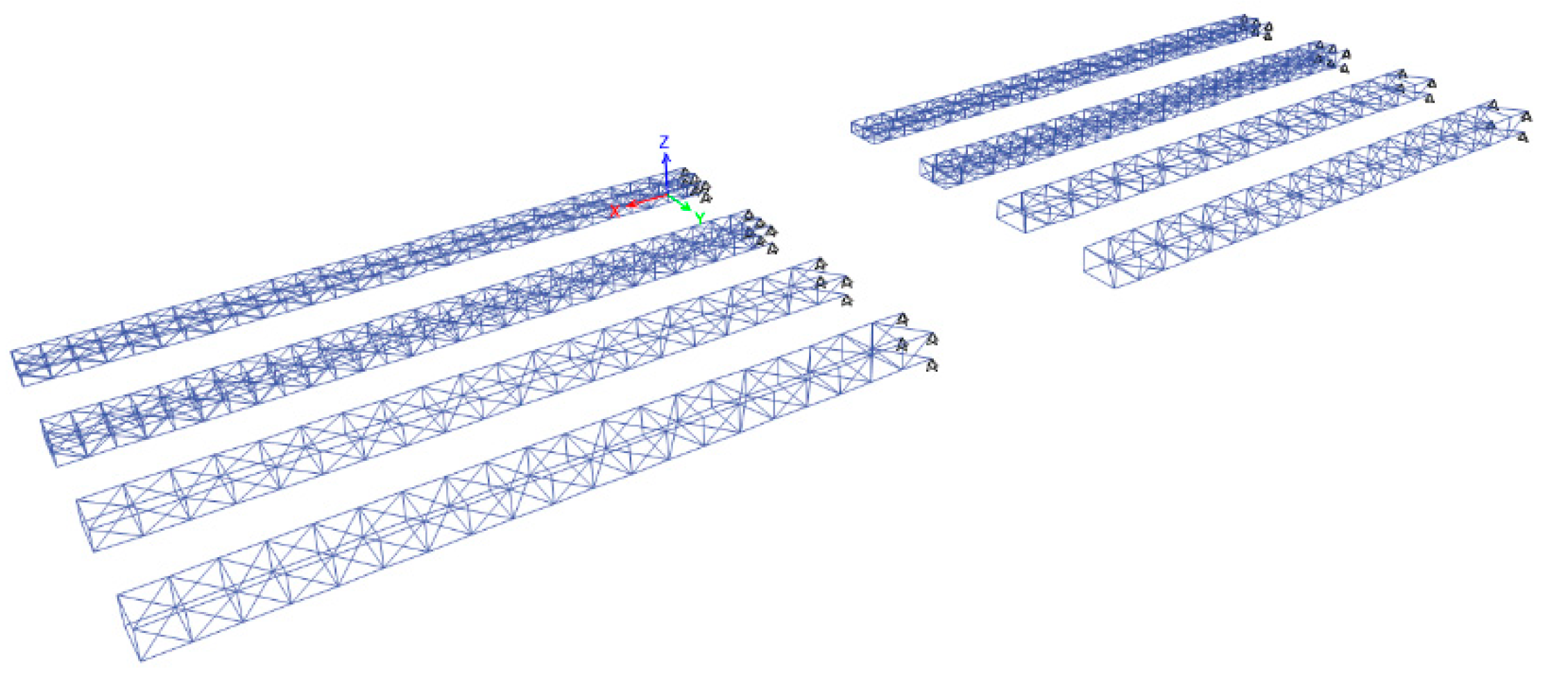
3. Floating Bridge Description
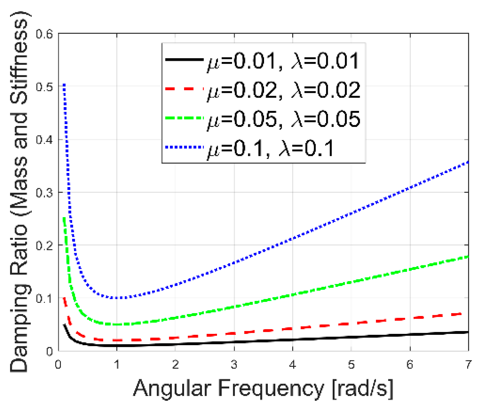
The deployment location of the floating bridge in this study is the coastal waters of Singapore, which are characterized as relatively shallow water with a water depth of 20 m and mild environmental conditions. Extreme sea conditions with a 100-year return period is taken as Hs = 2 m, Tp = 5.8 s. Long crested waves are studied. The water depth is 30 m. Since the focus is to find out different structural configuration effects and response properties. Other environmental load effects are not considered in this study.
Single curved bridges with two bridge total spans of 500 and 1000 m are the focus, with the same curve radius of 1000 m. The two bridges have the same rise-to-span ratio of 0.134. Discrete pontoons are used to support the bridge, with each pontoon supporting approximately 100 m of the bridge deck. The short bridge (500 m) includes four pontoons, while the long bridge (1000 m) has nine pontoons in total. The bridge deck is designed to have two ways, with three lanes in each way. The bridge cross-section is designed to be a truss configuration. The steel truss work forms the key structural component of the bridge. Figure 1 shows the two bridge configurations. The global coordinate system, local coordinate system, and pontoon positions are also shown. The local Y axis represents the weak axis of the bridge, while the local Z axis is the strong bridge axis. The two ends of the bridge are connected to the shore. Two types of end connections are investigated, i.e., rigid BC with all the six D.O.F fixed and flexible BC with rotational D.O.F regarding local Y and local Z free.
The pontoon supporting the bridges has an elliptic cylinder shape and 6 D.O.F rigid body motions as shown in Figure 2. The pontoons have uniform dimensions with the major axis length of 60 m, minor axis length of 22 m, and height of 9 m. The elliptic shape is expected to reduce the drag forces applied on the pontoon. These pontoons are evenly distributed along the bridge length, and the pontoon major axis is pointing to the global x direction. The center of gravity (C.O.G) of the pontoon is −2 m from the still water line (SWL), and the C.O.G of the bridge deck is 5 m from the SWL. The bridge deck weight distribution is estimated to be 3.99 Mkg/100 m. The stability of the pontoons was studied previously [27]. The dimensions and weight parameters of the pontoons and bridge deck are listed in Table 1.
A truss configuration is used in the bridge cross-section, resembling the Bergsøysund Bridge in Norway [28] but with different dimensions and bridge curvatures. To evaluate the bridge deck flexural rigidity EIy and EIz, and torsional rigidity GJ, which is about the local y, z and x axis, respectively, finite element models of truss work segments with various configurations and structural member sizes were developed using commercial software SAP2000 [29], as shown in Figure 3. Among these parameters, E is the Young’s modulus, A is the bridge’s cross-sectional area, I is the moment of inertia of the cross-sectional area, G is the shear modulus, and J is the torsional constant of the cross-section. Shear modulus and Young’s modulus have the relationship of G = E/2/(1 + ν), with Poisson ratio ν = 0.3. G = 76.92 GPa, E = 200 GPa. In the end, steel circular hollow sections with a diameter of 1200 mm for the main chord members and 800 mm for diagonal members are considered in this study, with EIy, EIz, and GJ values of 1.0 × 10⁷ MNm2, 2.0 × 10⁷ MNm2, and 1.0 × 10⁷ MNm2/rad, respectively. EA is taken as 1 × 10⁶ MN. Structural damping is also considered and is calculated by Rayleigh damping with the mass and stiffness proportional coefficients, then the damping ratio is calculated as ξ = 0.5(μ/ω + λ ω). With the variation of the coefficients μ and λ from 0.01 to 0.1, the damping ratio is plotted in Figure 4. It is seen that the damping ratio varies significantly. Focusing on the critical wave periods, which is around 2 s–10 s (0.628–3.14 rad/s) in this study, the parameters μ = 0.02 and λ = 0.02 induce damping ratios generally below 3% based on the estimation. This may be regarded as a reasonable assumption considering that other viscous effects, for example, from the wind and current, are not considered in the numerical model.

4. Numerical Model

Numerical modelling of the floating bridge involves both hydrodynamic and structural dynamic models, and these two models are coupled in one integrated model. Hydrodynamic properties of the pontoons as well as the structural properties of the bridge deck and the end connections are taken into consideration. Considering nonlinear features, such as viscous effects and structural geometrical nonlinearity, time domain analysis is needed.
Frequency domain hydrodynamic properties are calculated using the boundary element method [30] based on potential flow theory, followed by the transferring of these properties into the time domain. This method is called the hybrid time and frequency domain method [31,32], and is widely used in different offshore application studies [4,33,34,35,36,37,38,39,40]. In the case of strongly nonlinear hydrodynamic phenomenon, such as the slamming or green water problem [41], the linear hydrodynamic model is not suitable anymore. However, in this study, the linear hydrodynamic model is good enough, since there is no water entry and exit phenomena of the pontoons expected to occur. In the time domain, if r P T , r ˙ P T , and r ¨ P T are the displacement, velocity, and acceleration vectors of a pontoon, then the hydrodynamic forces applied on the pontoon can be expressed as:
F h y d = F e x t ( t ) A ( ) r ¨ P T ( t ) B ( ) r ˙ P T ( t ) 0 t k ( t τ ) r ˙ P T ( τ ) d τ C r ˙ P T ( t ) | r ˙ P T ( t ) | K r P T ( t )
where on the right hand side of the equation, the first term is the excitation force including Froude–Kryloff force due to the wave pressure distribution and diffraction force of the pontoon; the second to the fourth terms are forces due to radiation, in which the third term is the force due to the wave memory effect (retardation function force); the fifth term is due to the wave viscous effect, which is not considered in potential flow theory but is supposed to be considered in the time domain model; and the last term is the restoring force due to the pontoons’ vertical positions. More explanation is provided in the following.
The finite element method is used for the structural modelling of the bridge deck. The global dynamic equilibrium of the structural finite element formulation in time domain is expressed as [42]:
R I ( r , r ¨ , t ) + R D ( r , r ˙ , t ) + R S ( r , t ) = R E ( r , r ˙ , t ) ,
where r , r ˙ , and r ¨ are the displacement, velocity, and acceleration vectors for all the nodes in the FEM model; R I ( r , r ¨ , t ) is the inertia force vector of the nodes. It includes the bridge structural mass and pontoon mass. In addition, the added mass of the pontoons at infinite frequency as shown in Equation (1) can be considered. Therefore, the pontoon inertia term is expressed as ( M + A ( ) ) r ¨ P T ( t ) , where M is the pontoon structural mass matrix; A ( ) is the added mass matrix at infinite frequency; and r ¨ P T ( t ) is the pontoon acceleration, which is also the acceleration of the node, through which bridge element and pontoons are connected. The pontoon inertia forces are added in the inertia terms of the connecting node.
R S ( r , t ) is the stiffness force vector, including the structural internal stiffness of the bridge deck. In addition, the hydrostatic stiffness forces of the pontoons, like the inertia terms, are added to the stiffness terms of the connecting node. The hydrostatic stiffness of the pontoon is expressed as K r P T ( t ) , where K is the hydrostatic stiffness matrix, and r P T ( t ) is the pontoon displacement, which is also the displacement of the connecting node. The end connections of the bridge are also specified in the stiffness force vector.
R D ( r , r ˙ , t ) is the damping force vector, including the structural internal damping and infinite frequency wave radiation damping of the pontoons B ( ) r ˙ P T ( t ) ; and r ˙ P T ( t ) is the velocity of the pontoon, which also represents the velocity of the connecting node. It is noted that for floating structures with zero forward speed, B ( ) = 0 .
R E ( r , r ˙ , t ) is the external force vector. This term also includes forces that are not specified in the previous terms. In this study, those forces include the wave excitation forces, quadratic viscous forces, current forces, tidal variation-induced forces, and retardation forces. All these external applied forces are exerted on the pontoons. Note that the quadratic viscous forces are expressed as C r ˙ P T ( t ) | r ˙ P T ( t ) | , where C is the quadratic viscous damping coefficient matrix, in which the coefficients are set to 0.9 for surge and sway D.O.Fs of the pontoons, and 1.2 for the heave D.O.F [43]. The retardation force, as shown in Equation (1), is expressed by the convolution integral 0 t k ( t τ ) r ˙ P T ( τ ) d τ , where k ( τ ) is the retardation function matrix, and is expressed as:
k ( t ) = 2 π 0 [ B ( ω ) B ( ) ] cos ( ω t ) d ω = 2 π 0 ω [ A ( ω ) A ( ) ] sin ( ω t ) d ω ,
which tends to vanish with time.
In this study, the JONSWAP spectrum is used to describe the irregular wave condition or sea state. The JONSWAP spectrum is expressed as:
S ( ω ) = α g 2 ω 5 exp { 5 4 ( ω p ω ) 4 + ln γ exp [ 1 2 σ 2 ( ω ω 1 ) 2 ] } ,
where g = 9.81 ms−2; ω p is the peak frequency of the sea state; γ and σ are the spectral shape parameters, in which γ = 3.3 is used and σ = 0.07 when ω ω p , σ = 0.09 when ω > ω p ; and α is determined from the following equation:
α = 5.06 ( H s T p ) 2 ( 1 0.287 ln γ ) ,
where H s is the significant wave height, and T p is the spectral peak period. Once the sea state is determined, the JONSWAP spectrum can be used to generate the wave force spectrum from the wave force response amplitude operator; then, wave force time series are generated based on the superposition principle.
Several cases are specified and used in this investigation. The simulation cases are summarized in Table 2, where RS (Rigid B.Cs with Short bridge) and FS (Flexible B.Cs with Short bridge) represent the short 500-m bridge with rigid and flexible end connections, respectively, and RL (Rigid B.Cs with Long bridge) and FL (Flexible B.Cs with Long bridge) represent the 1000-m-long bridge. Rigid connection is fully rigid on the end connection, which represents the strong connections in the real structures. Flexible connection means the rotation D.O.F along the y and z directions (Ry and Rz) in the local coordinate system are set free.
The time domain calculation is carried out in SIMO-RIFLEX code, which was developed by Sintef Ocean (previously MARINTEK). SIMO [44] is a code to simulate marine operations involving various bodies in the time domain. RIFLEX [42] is a code for analysis of slender marine structures. It is a nonlinear time domain program with a finite element formulation that can handle large displacement and rotations.
The frequency domain hydrodynamic properties are calculated for the pontoon through the penal method in WADAM [45], generating the hydrodynamic excitation forces and added mass, potential damping, etc. Then, these data are transferred to the time domain through SIMO. The bridge deck girders are modelled in RIFLEX using beam elements. The pontoons are connected to the FEM model in RIFLEX through the connecting nodes [42]. Then, the wave loads are transferred to the FEM model. The FEM calculation is carried out in RIFLEX in the time domain, providing pontoon motion parameters, then these parameters are transferred to SIMO to update the wave loads applied on pontoons. Therefore, the model is the coupled hydro-structural dynamic model, in which the pontoon motion and bridge deck responses are calculated and updated at each time step. However, the pontoons are assumed to be rigid, and no hydroelasticity on the pontoons is considered, which means the hydrodynamic properties in the frequency domain are kept linear and unchanged in the coupled model. The calculation time step of 0.1 s is applied, and the Newmark method is used for numerical integration to solve the differential equation. Under irregular wave conditions, a time length of 4000 s of calculation is performed, and 3600 s (1 h) of steady-state simulation results are used for the analysis.

5. Numerical Results

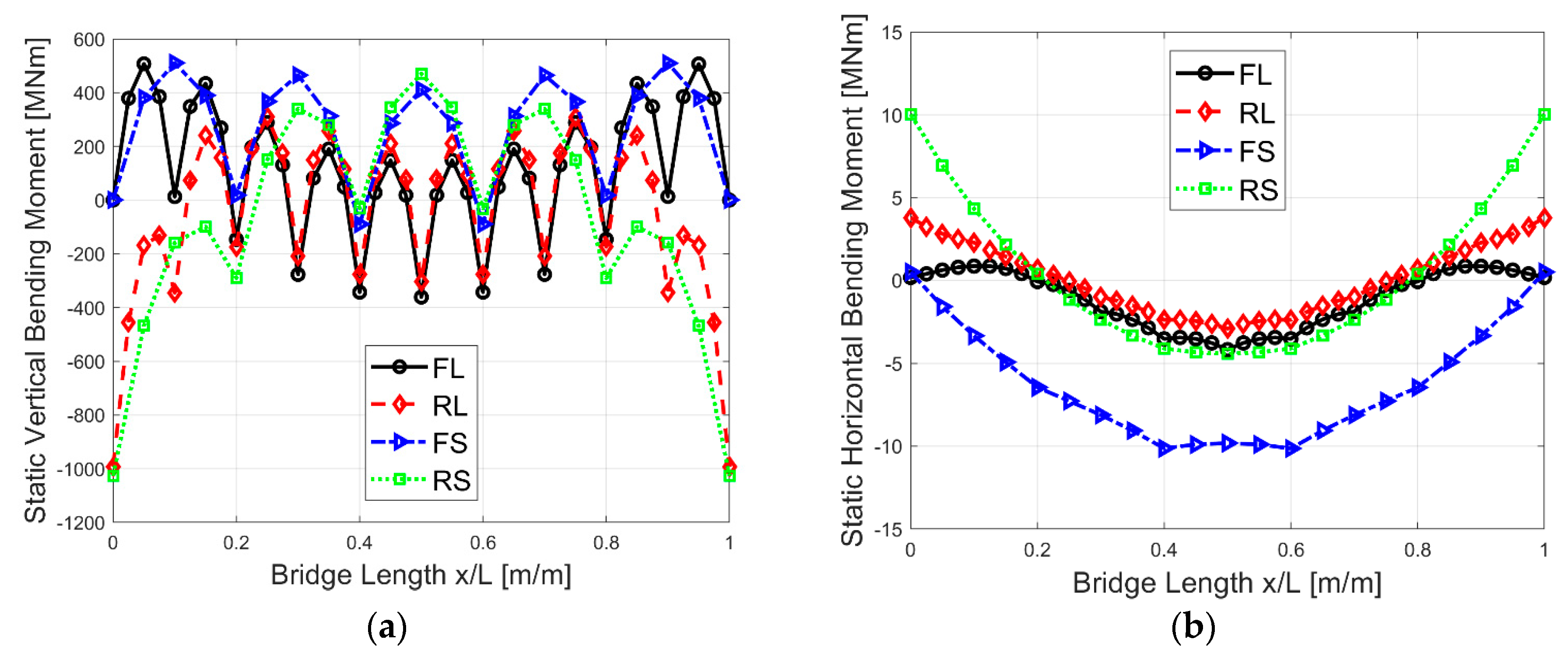
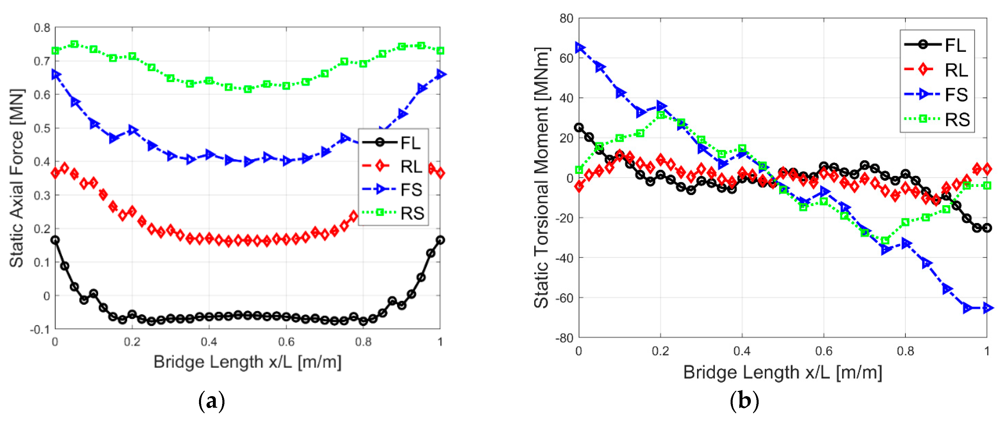
5.1. Static Responses

Figure 5 and Figure 6 present the static structural responses of the curved floating bridges with different B.Cs and span lengths. As for the vertical bending moment (Figure 5a), negative moment values were observed at both ends for bridges with rigid supports, and the magnitude is much larger than that of the positive moment at the mid-span. Compared to the short-span bridge cases, the long-span floating bridges own the same end negative moments but smaller positive moments in the middle, which are beneficial for future structural designs. In terms of the horizontal bending moment (Figure 5b), its magnitude is much smaller than that of the vertical moment, and the long-span bridge generally took less moment than the short-span bridge. Axial forces (Figure 6a) show some differences for the four cases. The reasons are due to different B.Cs and the uneven load distribution along the bridge length (differences between the bridge deck weight distribution and pontoon buoyancy force distribution). The torsional moment values are larger for bridge cases with flexible ends (Figure 6b).

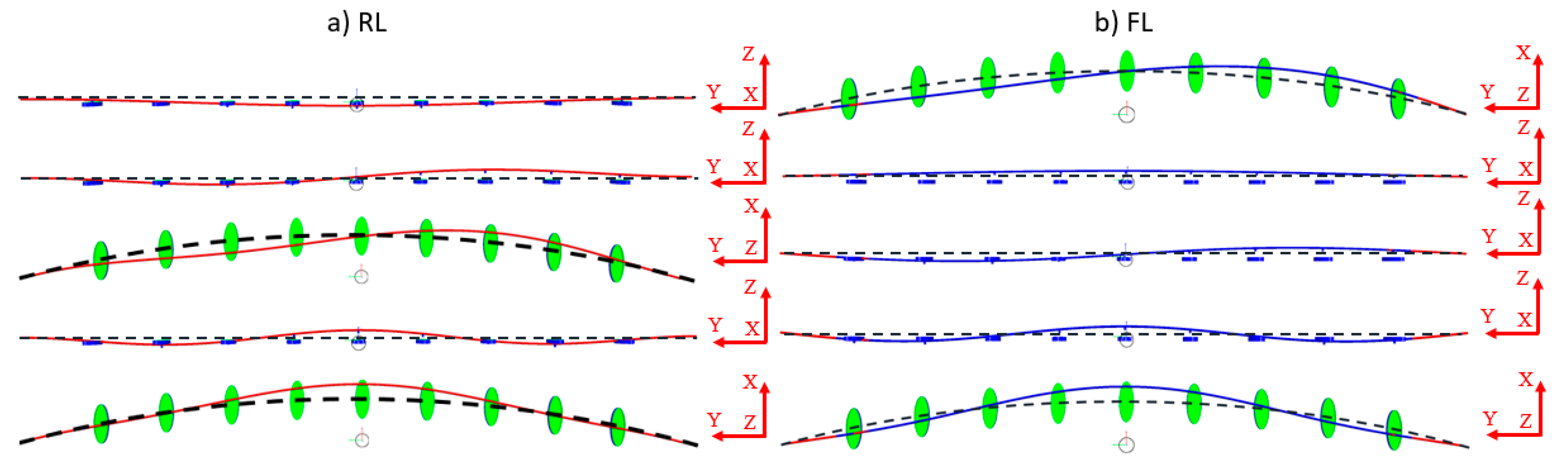
5.2. Eigen Value Analysis

Eigen value analysis was carried out to identify the eigen properties of the bridge with different B.Cs and total lengths. It is noted that only the added mass at infinite frequency (constant value) rather than its variation with frequency was considered. This may have introduced limited uncertainties. The uncertainties due to this simplification were addressed as follows: For the 4600-m-long floating bridge with discrete pontoons [38], the largest error with and without considering the frequency-dependent added mass is 10% for the first eigen period of around 57 s, while for the subsequent eigen period, the error varies from around 0.1% to 7%. In this study, the largest first eigen period is around 10s (shown later), which means the bridge is much stiffer than the 4600-m bridge. In this case, the mass effect on the eigen period is significantly less, indicating the uncertainties due to neglecting the added mass variation with frequency are quite limited.
The first 15 eigen periods are listed in Table 3. It is obvious that the largest eigen period corresponds to the softest bridge configuration, which is case FL. The value for the first eigen mode is 9.63 s for case FL, followed by 7.77 s for case RL, 7.36 s for case FS, and 6.03 s for case RS. The following eigen modes generally have the same trends. This trend shows that the softness of the bridge is most significantly influenced by the length for these two bridges. The data also show that for the long bridge, the eigen values decrease much slower than that for the short bridge, which means more eigen modes will be excited for the long bridge under the same excitation spectrum. It is noted that the Rayleigh damping is used in this study, so the damping ratios vary with the eigen periods. Considering that the first several eigen modes contribute significantly to the dynamic responses, damping ratios based on the first five eigen periods were calculated to be in the range of 2.2%–4.3%, with mass and stiffness proportional coefficients of 0.02, which is in a reasonable range. This damping level will not affect the dynamic responses significantly, which indicate negligible uncertainties due to damping coefficients.
The first five eigen mode shapes are plotted in Figure 7 and Figure 8. The first mode shapes are like simply supported and fixed beams, and except for case FL, the first mode shape is in the horizontal plane (X-Y plane). The other mode shapes are also like that of simple beams, as expected. The dynamic responses will be the superposition of the first dominant mode shapes with different weighting factors.

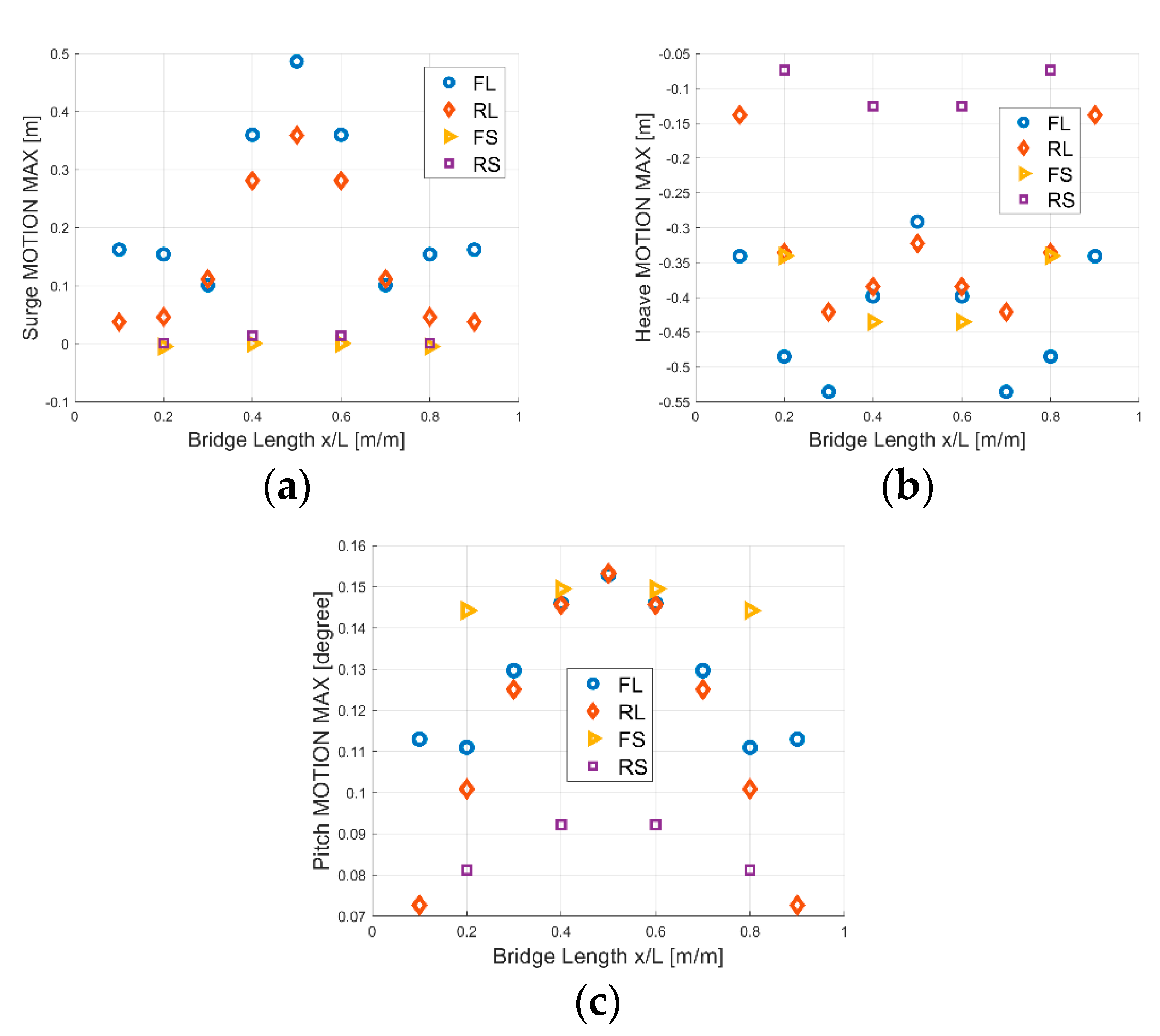
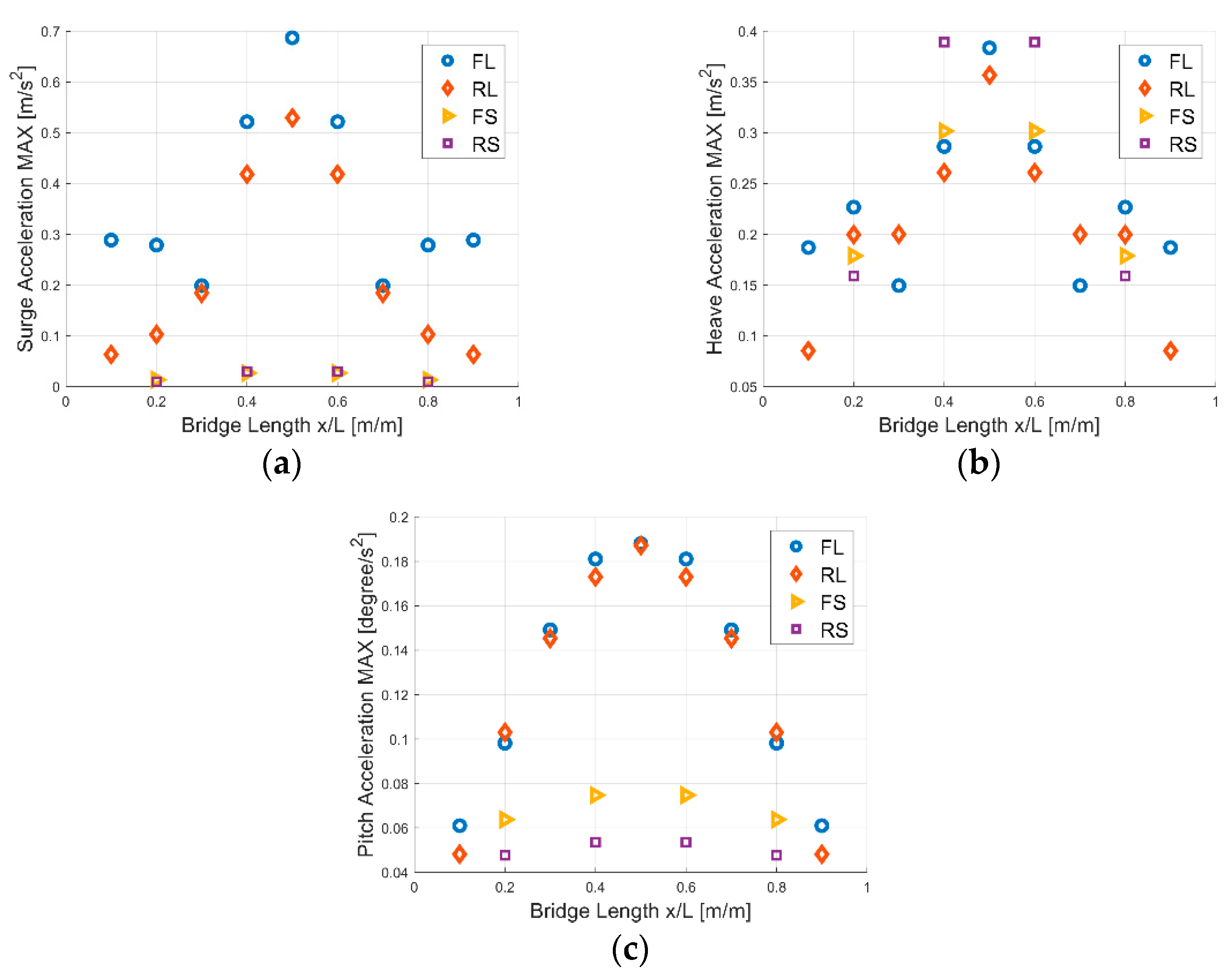
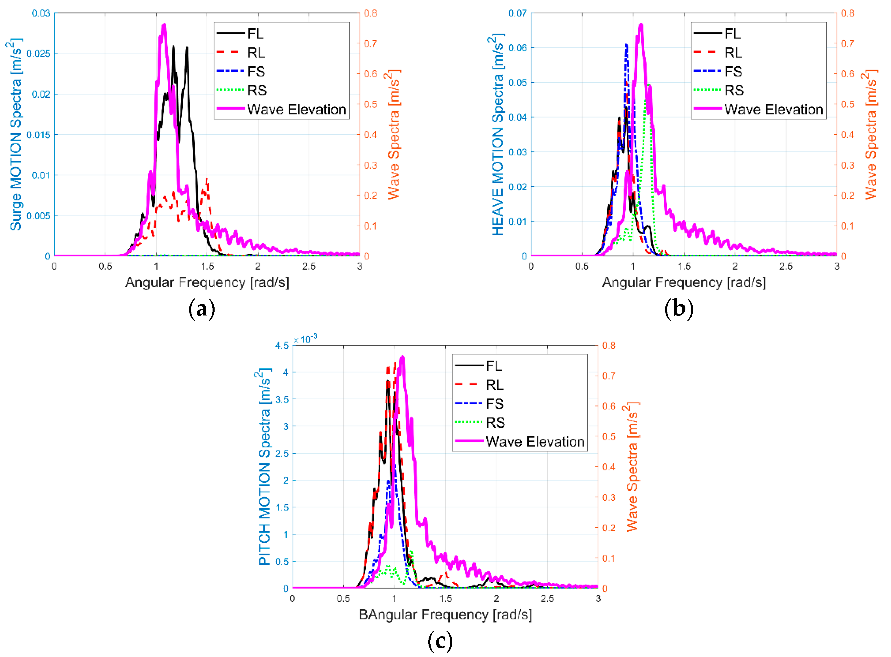
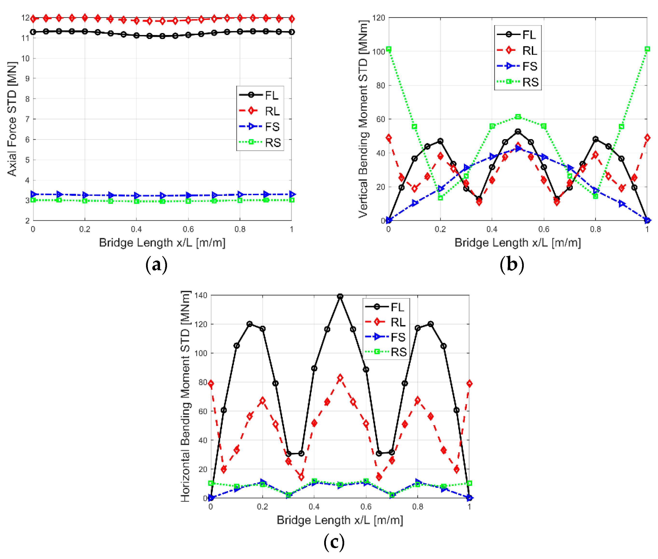
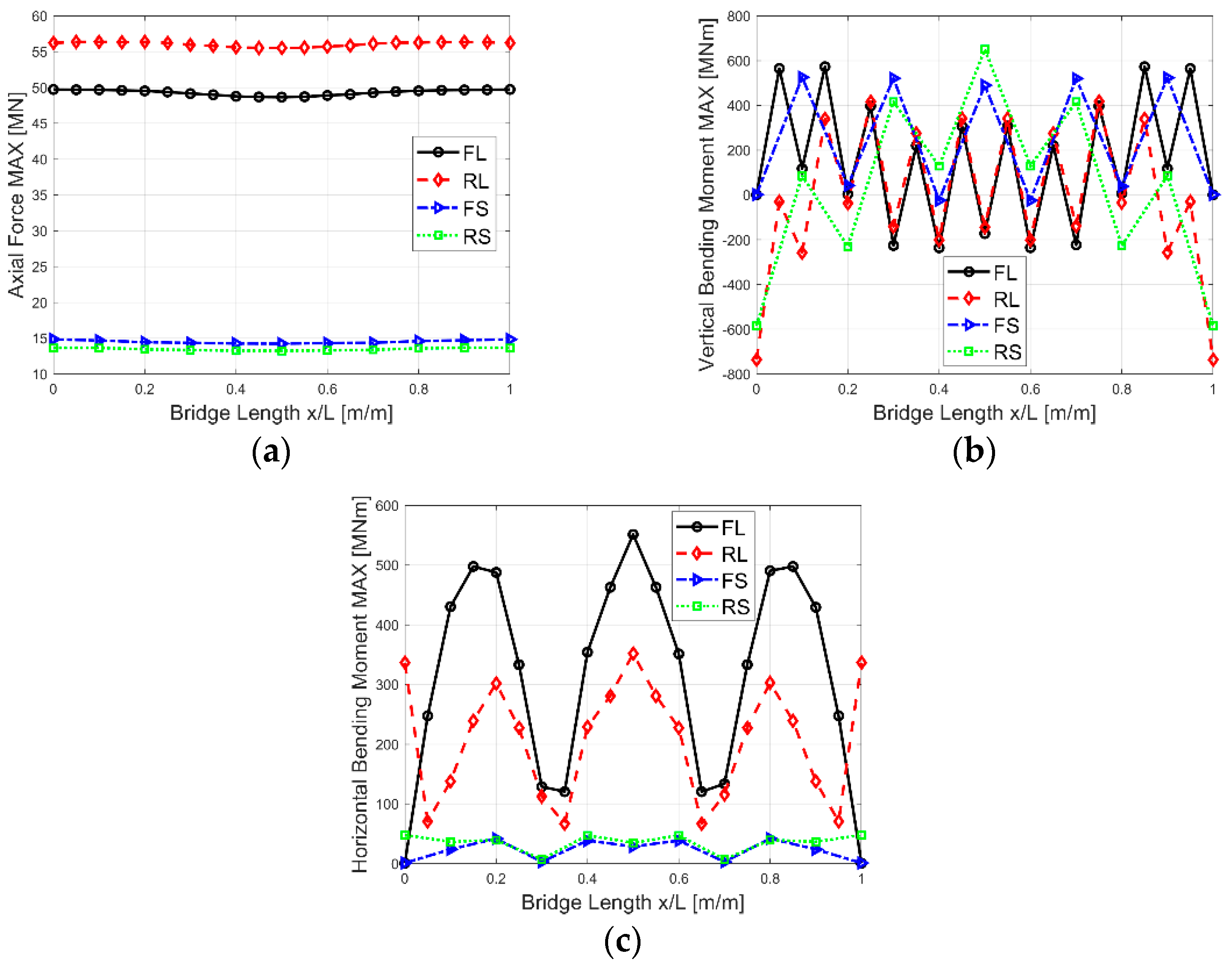
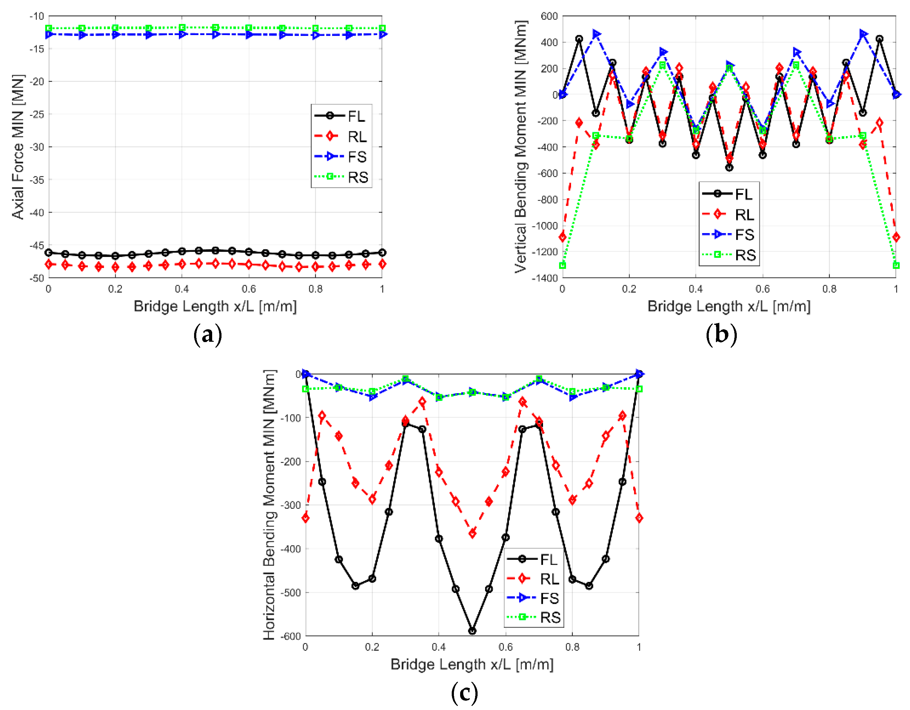
5.3. Irregular Wave Analysis

Bridge responses under irregular wave actions can to some extent reflect the real performance. In this study, the current and wind effects were considered marginally important, so were not included. Homogeneous wave conditions were assumed, which means the irregular wave forces applied on all the pontoons are the same.
The 100-year return period storm with Hs = 2m and Tp = 5.8 s was used in the irregular wave analysis. There was no repetition of the simulation, as only one seed number was used, and the wave was coming in one direction as shown in Figure 2. By irregular wave analysis, the pontoon motion, bridge deck structural response distribution along the bridge length, and response properties could be investigated. The results show the real performance of the bridge under extreme conditions. Based on 1-h of steady-state simulation, the statistical values and spectral results are presented.
Pontoon motions and accelerations directly affect the driving comfort and serviceability of the floating bridges. Under operational conditions, the wave-induced deflection should not exceed ±0.3 m in both the surge and heave, and ±0.5 degree in pitch, while the acceleration induced by the wave should not exceed ±0.5 m/s2, ±0.5 m/s2, and ±0.05 rad/s2 (±2.87 degree/s2) in the surge, heave, and pitch, respectively [25]. Under survival conditions, the structural responses should not exceed the capacity of the structure.
The pontoon motion Maximum (MAX) and Standard Deviation (STD) values along the bridge length are shown in Figure 9 and Figure 10. The pontoon acceleration MAX values along the bridge are shown in Figure 11. The spectral results of the surge, heave, and pitch motions of pontoon number 4 (PT4) for the long bridge and pontoon number 2 (PT2) for the short bridge (both located at 0.4 L position) are shown in Figure 12.
From Figure 9 and Figure 10, both surge and pitch responses for cases FL and RL are significantly larger than that for cases FS and RS. It is noted that the maximum values are also affected by the static deflection under bridge deck weight, so STD values can more properly reflect the dynamic effects. It can also be observed that for the RL case, the surge motion is significantly reduced compared with the FL case, while for the FS and RS cases, the surge STDs are similar, which means the BC strongly affects the surge motions for the 1000-m bridge. The reason could be due to the modes that are excited, because the fifth eigen mode of FL is 4.75 s (1.32 rad/s), which is close to the excitation periods and is in the X-Y plane, while eigen periods of 1.82 s (3.47 rad/s, RS) and 2.42 s (2.60 rad/s, FS) correspond to the horizontal eigen modes of the short bridges far away from excitation. This can also be observed in the surge spectra in Figure 12.
The heave motion responses are similar for the four simulation cases. By looking at the eigen periods, they all have vertical modes (global Y-Z plane) located in the wave region, which is also reflected in Figure 12. For the pitch motion, the effects from BC are not so significant for long bridges but are important for short bridges, inducing a larger pitch for FS. There are also significant influences from the bridge length to pitch motion. From the pitch spectra, it is seen that several eigen modes are involved, especially the modes close to 0.9 rad/s. The acceleration plots in Figure 11 also show similar trends with Figure 10, and the acceleration MAX values reflect the driving comfort. Even under the extreme sea state, the acceleration MAX values mostly do not exceed the guideline values.
Figure 13, Figure 14 and Figure 15 show the STD, MAX, and Minimum(MIN) values of the internal forces along the bridge length, including the axial force, vertical bending moment, and horizontal bending moment. Compared with the static results, the axial forces under wave actions are significantly larger. While being similar to the static results, the negative vertical bending moments under wave actions occur at ends of RL and RS, and the magnitudes of the negative moments are larger than the positive moment values in the mid-span location, which should be handled with caution in the structural design. In addition, a shorter span length (RS and FS) usually results in relatively larger positive vertical moments (middle of Figure 14 and middle of Figure 15), and rigid-end connections (RL and RS) also introduce large end values. On the contrary, much more significant horizontal bending moment values are obtained for long-span bridges (FL and RL) as compared to short spans (right of Figure 14 and right of Figure 15), in terms of STD, MAX, and MIN. This indicates that the arch effect (external loads transfer to the axial force rather than bending moment) is not so obvious, especially for the long bridge. In further structural design and optimization, it is suggested to increase the rise-span ratio or increase the horizontal stiffness of long-span bridge cases while the vertical stiffness can be slightly reduced.
Figure 16 and Figure 17 present the correlation between the axial force and horizontal bending moments (represented by the 1-h time series of various positions along the bridge length, e.g., 0.1 L, 0.2 L, etc.) for curved bridges with different span lengths and B.Cs. It is noted that only the half-length of the bridge was analyzed due to the symmetrical properties. Different trends of the axial force (N)-horizontal bending moment (Mz) couple effects were observed at different sections of the bridges with the varying span length and B.Cs. For instance, the distribution of the N-Mz points of the FL bridge changes from a horizontal line to inclined lines as the distance from the end support to the section increases (left of Figure 16 and left of Figure 17), while an opposite trend is observed for the RL bridge (right of Figure 16 and right of Figure 17).
The N-Mz coupling trends indicate the arch effect in the horizontal curved bridge when subjected to wave loads. It is observed that the ratio of the maximum bending moment to the maximum axial force is larger for the long bridge than the short bridge, indicating the arch effect is less significant for the long bridge compared with the short one. The maximum horizontal moment changes at different locations while the maximum axial force almost remains constant. Although N-Mz points scatter in different quadrants, fairly clear boundaries are seen in Figure 16 and Figure 17 as left and right vertical lines, and the critical N-Mz point can be utilized for further section designs.
The spectral results for the axial force, and horizontal and vertical bending moments at the bridge deck position of 0.4 L are shown in Figure 18. The axial forces and horizontal bending moments for the short bridge are much smaller than the long bridge, which is confirmed in Figure 13, Figure 14 and Figure 15, and differences between FL and RL are mainly due to various eigen modes. It is also seen that most response peaks are located at the wave region, which is due to the first several eigen periods that are close to the spectral period.

6. Conclusions and Discussion

This paper investigated curved floating bridges with a same small rise-span ratio. Different bridge lengths of 500 and 1000 m were studied. Varied B.Cs were also investigated. Static, eigen value, and dynamic analysis were carried out for the four different cases. Pontoon motions and structural reaction forces and moments were presented and analyzed. The motion responses indicated the satisfaction of the survivability criteria for the bridge configuration under the operational and extreme sea states. In this study, only the extreme sea state was studied to focus on the structural response properties under different bridge configurations. The structural reaction results showed that although the same rise-span ratio was applied, bridges with different lengths have various response properties, and the short bridge provides a prominent arch effect compared to the long bridge. In addition, the response properties provide insights into further structural design. Based on the investigation, the following conclusions can be drawn.
Eigen value analysis considers the infinite frequency added mass rather than the frequency-dependent added mass, which involves uncertainties, but these uncertainties are quite limited. The eigen periods showed that the softest bridge configuration is FL, followed by RL, FS, and RS. The eigen values were varied from 0.3 s to around 10 s. For the long bridge, eigen values decreased much slower than that for the short bridge, which means more eigen modes will be excited for the long bridge under the same excitation spectrum. Negative end moments were induced for the RL and RS bridge cases in static conditions, and the negative vertical moment value was much larger than the horizontal one. When compared to short-span bridge cases (FS and RS), a smaller positive moment was observed in the middle span of FL and RL, which is beneficial for structural design.
Irregular wave analysis was performed under the extreme sea state. The pontoon motions showed that BC strongly affected the surge motions for the 1000-m bridge, because it varied the eigen periods, i.e., the resonant region; another reason may be due to the relatively flexible properties of the long bridge, which highlights the importance of the BC. The heave motion responses were similar for the four simulation cases and frequencies were in the wave region. For pitch motions, there were significant influences from the bridge length. The acceleration MAX values mostly did not exceed the guideline values of the operational condition even under the extreme sea state, which indicates that the motion of the bridges under wave action is acceptable.
From the structural responses, it can be concluded that flexible end connections are better, considering the vertical and horizontal end bending moment. Short bridges are better in terms of the axial forces and horizontal bending moment, while long bridges have relatively lower vertical bending moments. In further structural design and optimization, it is suggested to increase the horizontal stiffness of long-span bridge cases while the vertical stiffness can be slightly reduced.
The bending effect was apparently observed in the current research study on the shallow curved floating bridge with a small rise-to-span ratio (0.134). It is not a preferable force state for an arch bridge geometry, where the axial compression effect is still prominent. However, the short bridge showed a greater arch effect than the long bridge. Therefore, larger rise-to-span ratios are to be considered in a companion paper to explore the optimal rise-to-span ratios for curved floating bridges and the coupling N-M effect will be further studied.

Author Contributions

Conceptualization, L.W., D.J. and J.D.; Methodology, L.W., D.J. and J.D.; Software, L.W.; Validation, L.W., D.J. and J.D.; Formal analysis, L.W., D.J.; Investigation, L.W., D.J.; Resources, L.W., D.J. and J.D.; Data curation, L.W., D.J. and J.D.; Writing—original draft preparation, L.W., D.J.; Writing—review and editing, L.W., D.J. and J.D.; Visualization, L.W.; Supervision, L.W., D.J. and J.D.; Project administration, L.W. and D.J.; Funding acquisition, L.W., D.J. All authors have read and agreed to the published version of the manuscript

Funding

This research was funded by Natural Science Foundation of Jiangsu Province, grant No. BK20180487; National Natural Science Foundation of China (NSFC), grant No.51808292; Research funds from Newcastle University through Newcastle Research & Innovation Institute Pte Ltd. (NewRIIS), Singapore; And research funds from State Key Laboratory of Hydraulic Engineering Simulation and Safety, Tianjin University, Grant number: HESS-1709. The aforementioned funds are gratefully acknowledged.

Conflicts of Interest

The authors declare no conflict of interest.

References

  1. Jiang, D.; Tan, K.; Ong, K.; Heng, S.; Dai, J.; Lim, B.; Ang, K. Behavior of prestressed concrete self-stabilizing floating fuel storage tanks. In Proceedings of the 4th Congrès International de Géotechnique–Ouvrages–Structures, Ho Chi Minh City, Vietman, 26–27 October 2017; pp. 1097–1106. [Google Scholar]
  2. Jiang, D.; Tan, K.H.; Dai, J.; Ong, K.C.G.; Heng, S. Structural performance evaluation of innovative prestressed concrete floating fuel storage tanks. Struct. Concr. 2019, 20, 15–31. [Google Scholar] [CrossRef]
  3. Jiang, D.; Tan, K.H.; Wang, C.M.; Ong, K.C.G.; Bra, H.; Jin, J.; Kim, M.O. Analysis and design of floating prestressed concrete structures in shallow waters. Mar. Struct. 2018, 59, 301–320. [Google Scholar] [CrossRef]
  4. Wan, L.; Han, M.; Jin, J.; Zhang, C.; Magee, A.R.; Hellan, Ø.; Wang, C.M. Global dynamic response analysis of oil storage tank in finite water depth: Focusing on fender mooring system parameter design. Ocean Eng. 2018, 148, 247–262. [Google Scholar] [CrossRef]
  5. Zhang, C.; Wan, L.; Magee, A.R.; Han, M.; Jin, J.; Ang, K.K.; Hellan, Ø. Experimental and numerical study on the hydrodynamic loads on a single floating hydrocarbon storage tank and its dynamic responses. Ocean Eng. 2019, 183, 437–452. [Google Scholar] [CrossRef]
  6. Dai, J.; Ang, K.K.; Jin, J.; Wang, C.M.; Hellan, Ø.; Watn, A. Large floating structure with free-floating, self-stabilizing tanks for hydrocarbon storage. Energies 2019, 12, 3487. [Google Scholar] [CrossRef] [Green Version]
  7. Watanabe, E.; Wang, C.; Utsunomiya, T.; Moan, T. Very large floating structures: Applications, analysis and design. Core Rep. 2004, 2, 104–109. [Google Scholar]
  8. Watanabe, E.; Utsunomiya, T. Analysis and design of floating bridges. Prog. Struct. Eng. Mater. 2003, 5, 127–144. [Google Scholar] [CrossRef]
  9. Kashiwagi, M. Research on Hydroelastic Responses of VLFS: Recent Progress and Future Work. In Proceedings of the Ninth International Offshore and Polar Engineering Conference, Brest, France, 30 May–4 June 1999. [Google Scholar]
  10. Watanabe, E.; Utsunomiya, T.; Wang, C. Hydroelastic analysis of pontoon-type VLFS: A literature survey. Eng. Struct. 2004, 26, 245–256. [Google Scholar] [CrossRef]
  11. Fu, S.; Cui, W.-C.; Chen, X.; Wang, C. Hydroelastic analysis of a nonlinearly connected floating bridge subjected to moving loads. Mar. Struct. 2005, 18, 85–107. [Google Scholar]
  12. Watanabe, E.; Utsunomiya, T.; Wang, C.M.; Xiang, Y. Hydroelastic Analysis of Pontoon-type Circular VLFS. In Proceedings of the Thirteenth International Offshore and Polar Engineering Conference, Honolulu, HI, USA, 25–30 May 2003. [Google Scholar]
  13. Seif, M.S.; Inoue, Y. Dynamic analysis of floating bridges. Mar. Struct. 1998, 11, 29–46. [Google Scholar] [CrossRef]
  14. Xu, Y.; Øiseth, O.; Moan, T. Time Domain Modelling of Frequency Dependent Wind and Wave Forces on a Three-span Suspension Bridge with two Floating Pylons Using State Space Models. In Proceedings of the ASME 36th International Conference on Ocean, Offshore and Arctic Engineering, Trondheim, Norway, 25–30 June 2017. [Google Scholar]
  15. Petersen, Ø.W.; Øiseth, O. Sensitivity-based finite element model updating of a pontoon bridge. Eng. Struct. 2017, 150, 573–584. [Google Scholar] [CrossRef] [Green Version]
  16. Løken, A.; Oftedal, R.; Aarsnes, J. Aspects of Hydrodynamic Loading and Responses in Design of Floating Bridges. In Proceedings of the Second Symposium on Strait Crossings, Trondheim, Norway, 10 June 1990; pp. 10–13. [Google Scholar]
  17. Solland, G.; Haugland, S.; Gustavsen, J.H. The Bergsøysund Floating Bridge, Norway. Struct. Eng. Int. 1993, 3, 142–144. [Google Scholar] [CrossRef]
  18. Cheng, Z.; Svangstu, E.; Gao, Z.; Moan, T. Field measurements of inhomogeneous wave conditions in Bjørnafjorden. J. Waterw. PortCoast. Ocean Eng. 2018, 145, 05018008. [Google Scholar] [CrossRef] [Green Version]
  19. Cheng, Z.; Gao, Z.; Moan, T. Wave load effect analysis of a floating bridge in a fjord considering inhomogeneous wave conditions. Eng. Struct. 2018, 163, 197–214. [Google Scholar] [CrossRef]
  20. Dai, J.; Leira, B.J.; Moan, T.; Kvittem, M.I. Inhomogeneous wave load effects on a long, straight and side-anchored floating pontoon bridge. Mar. Struct. 2020, 72, 102763. [Google Scholar] [CrossRef]
  21. Istrati, D.; Buckle, I.G. Effect of Fluid-structure Interaction on Connection Forces in Bridges Due to Tsunami Loads. In Proceedings of the 30th US-Japan Bridge Engineering Workshop, Washington, DC, USA, 21–23 October 2014. [Google Scholar]
  22. Higgins, C.; Lehrman, J.; Bradner, C.; Schumacher, T.; Cox, D. Hybrid Testing of a Prestressed Girder Bridge to Resist Wave Forces. In Proceedings of the 29th US-Japan bridge engineering workshop, Tsukuba, Japan, 11–13 November 2013. [Google Scholar]
  23. Sha, Y.; Amdahl, J. Numerical investigations of a prestressed pontoon wall subjected to ship collision loads. Ocean Eng. 2019, 172, 234–244. [Google Scholar] [CrossRef]
  24. Sha, Y.; Amdahl, J.; Dørum, C. Local and Global Responses of a Floating Bridge Under Ship–Girder Collisions. J. Offshore Mech. Arct. Eng. 2019, 141, 031601. [Google Scholar] [CrossRef]
  25. Lwin, M. Floating bridges. Bridge Eng. Handb. 2000, 22, 1–23. [Google Scholar]
  26. The ISSC Committee VI.2. Very Large Floating Structures. In Proceedings of the 16th International Ship and Offshore Structures Congress, Southampton, UK, 20–25 August 2006. [Google Scholar]
  27. Wan, L.; Magee, A.R.; Hellan, Ø.; Arnstein, W.; Ang, K.K.; Wang, C.M. Initial Design of a Double Curved Floating Bridge and Global Hydrodynamic Responses under Environmental Conditions. In Proceedings of the ASME 2017 36th International Conference on Ocean, Offshore and Arctic Engineering, OMAE2017-61802, Trondheim, Norway, 25–30 June 2017. [Google Scholar]
  28. Kvåle, K.A.; Sigbjörnsson, R.; Øiseth, O. Modelling the stochastic dynamic behaviour of a pontoon bridge: A case study. Comput. Struct. 2016, 165, 123–135. [Google Scholar] [CrossRef]
  29. Computers & Structures, Inc. CSI Analysis Reference Manual, rev. 15. Berkeley, CA, USA, July 2016; Available online: https://wiki.csiamerica.com/display/doc/CSI+Analysis+Reference+Manual (accessed on 10 May 2019).
  30. Faltinsen, O.M. Sea Loads on Ships and Offshore Structures; Cambridge University Press: Cambridge, UK, 1993; Volume 1. [Google Scholar]
  31. Naess, A.; Moan, T. Stochastic Dynamics of Marine Structures; Cambridge University Press: Cambridge, UK, 2013. [Google Scholar]
  32. Cummins, W. The impulse response function and ship motions. Schiffstechnik 1962, 47, 101–109. [Google Scholar]
  33. Wan, L.; Gao, Z.; Moan, T.; Lugni, C. Experimental and numerical comparisons of hydrodynamic responses for a combined wind and wave energy converter concept under operational conditions. Renew. Energy 2016, 93, 87–100. [Google Scholar] [CrossRef]
  34. Wan, L.; Gao, Z.; Moan, T. Experimental and numerical study of hydrodynamic responses of a combined wind and wave energy converter concept in survival modes. Coast. Eng. 2015, 104, 151–169. [Google Scholar] [CrossRef] [Green Version]
  35. Karimirad, M.; Moan, T. A simplified method for coupled analysis of floating offshore wind turbines. Mar. Struct. 2012, 27, 45–63. [Google Scholar] [CrossRef]
  36. Gao, Z.; Moan, T.; Wan, L.; Michailides, C. Comparative numerical and experimental study of two combined wind and wave energy concepts. J. Ocean Eng. Sci. 2016, 1, 36–51. [Google Scholar] [CrossRef] [Green Version]
  37. Michailides, C.; Gao, Z.; Moan, T. Experimental and numerical study of the response of the offshore combined wind/wave energy concept SFC in extreme environmental conditions. Mar. Struct. 2016, 50, 35–54. [Google Scholar] [CrossRef]
  38. Cheng, Z.; Gao, Z.; Moan, T. Hydrodynamic load modeling and analysis of a floating bridge in homogeneous wave conditions. Mar. Struct. 2018, 59, 122–141. [Google Scholar] [CrossRef]
  39. Wu, M.; Moan, T. Linear and nonlinear hydroelastic analysis of high-speed vessels. J. Ship Res. 1996, 40, 149–163. [Google Scholar]
  40. Kashiwagi, M. Transient responses of a VLFS during landing and take-off of an airplane. J. Mar. Sci. Technol. 2004, 9, 14–23. [Google Scholar] [CrossRef]
  41. Wan, L.; Greco, M.; Lugni, C.; Gao, Z.; Moan, T. A combined wind and wave energy-converter concept in survivalmode: Numerical and experimental study in regular waves with afocus on water entry and exit. Appl. Ocean Res. 2017, 63, 200–216. [Google Scholar] [CrossRef]
  42. Marintek. Riflex Theory Manual v4.0 Rev3. 2013. Available online: https://www.manualslib.com/products/Lexicon-Lx-Rev-3-2622504.html (accessed on 10 May 2019).
  43. DNV. Recommended Practice Dnv-rp-c205, Environmental Conditions and Environmental Loads. 2010. Available online: https://rules.dnvgl.com/docs/pdf/dnv/codes/docs/2010-10/rp-c205.pdf (accessed on 10 May 2019).
  44. Marintek. SIMO—Theory Manual Version 3.6, Rev: 2. 2009. Available online: https://projects.dnvgl.com/sesam/status/Simo/SIMO-release-notes_4.16.0.pdf (accessed on 10 May 2019).
  45. DNV. Wave Analysis by Diffraction and Morison Theory (WADAM), Sesam User Manual. V8.3. 2011. Available online: https://home.hvl.no/ansatte/tct/FTP/V2020%20Hydrodynamikk/Sesam/SESAM%20UM%20Brukermanualer/Wadam_UM.pdf (accessed on 10 May 2019).
Figure 1. Floating bridge configurations.
Jmse 08 00467 g001
Figure 2. Elliptic cylinder pontoon supporting the bridge, and the modes of the rigid body motion.
Jmse 08 00467 g002
Figure 3. Numerical model of various bridge girder cross-sections.
Jmse 08 00467 g003
Figure 4. Rayleigh damping ratios for various angular frequencies under different mass proportional coefficients µ and stiffness proportional coefficients λ.
Jmse 08 00467 g004
Figure 5. Static vertical (a) and horizontal (b) bending moment under the bridge’s self-weight for different cases.
Jmse 08 00467 g005
Figure 6. Static axial force (a) and torsional moment (b) under the bridge’s self-weight for different cases.
Jmse 08 00467 g006
Figure 7. First five eigen mode shapes for the floating bridge for RS (a) and FS (b) cases. (RS: Rigid B.Cs with Short Bridge; FS: Flexible B.Cs with Short bridge.).
Jmse 08 00467 g007
Figure 8. First five eigen mode shapes for the floating bridge for RL (a) and FL (b) cases. (RL: Rigid B.Cs with Long Bridge; FL: Flexible B.Cs with Long bridge.).
Jmse 08 00467 g008
Figure 9. Pontoon surge (a), heave (b), and pitch (c) motion maximum values’ distribution along the bridge length.
Jmse 08 00467 g009
Figure 10. Pontoon surge (a), heave (b), and pitch (c) motion standard deviation (STD) distribution along the bridge length.
Jmse 08 00467 g010
Figure 11. Pontoon surge (a), heave (b), and pitch (c) acceleration maximum values’ distribution along the bridge length.
Jmse 08 00467 g011
Figure 12. Spectral response of the surge (a), heave (b), and pitch (c) motions as well as the wave spectrum for different cases.
Jmse 08 00467 g012
Figure 13. Axial force (a), vertical moment (b), and horizontal moment (c) Standard Deviation (STD) distribution along the bridge length.
Jmse 08 00467 g013
Figure 14. Axial force (a), vertical moment (b), and horizontal moment (c) maximum values’ distribution along the bridge length.
Jmse 08 00467 g014
Figure 15. Axial force (a), vertical moment (b) and horizontal moment (c) minimum values distribution along bridge length.
Jmse 08 00467 g015
Figure 16. Correlation between the axial force and horizontal bending moment for the long-span curved bridge cases FL (a) and RL (b), represented by the 1-h time series of various positions along the bridge length (half-length due to symmetry).
Jmse 08 00467 g016
Figure 17. Correlation between the axial force and horizontal bending moment for the short-span curved bridge cases FS (a) and RS (b), represented by the 1-h time series of various points along the bridge length (half-length due to symmetry).
Jmse 08 00467 g017
Figure 18. Spectral response of the axial force (a), and vertical (b) and horizontal bending moment (c) at the 0.4 L position, as well as the wave spectrum for different cases.
Jmse 08 00467 g018
Table 1. Pontoon and bridge deck parameters.
Bridge Total Span L500/1000 (m)
Pontoon Number4/9
Pontoon Overall Dimension (Elliptic Cylinder)60 × 22 × 9 (m)
Pontoon Draft6 (m)
Pontoon C.O.G(0, 0, −2) (m)
GM (Horizontal and Longitudinal)3 and 35.5 (m)
Pontoon mass2.319 (Mkg)
Pontoon rotational Inertia Ixx, Iyy and Izz145.39, 660.29 and 721.03 (Mkg m2)
Bridge Deck C.O.G(0, 0, 5) (m)
Bridge Deck Weight3.990 (Mkg/100 m)
Table 2. Cases for the bridge deck’s cross-sectional rigidity and boundary conditions.
CasesTotal Span
(m)
EIy
(× 106 MNm2)
EIzv
(× 106 MNm2)
EA
(× 106 MN)
GJ
(× 106 MNm2/rad)
Boundary Conditions (B.Cs)
RS5001020110Fixed at 6 D.O.Fs
RL10001020110
FS5001020110Fixed at Translational D.O.F
Free at Ry and Rz, fixed at Rx
FL10001020110
Table 3. The first 15 eigen periods (unit: s) for the floating bridge under different B.Cs and total lengths.
LengthCases123456789101112131415
1000(m)RL7.776.846.135.184.283.672.822.632.611.961.901.541.441.281.27
FL9.637.927.446.054.754.373.253.092.632.392.241.711.531.441.36
500 (m)RS6.033.101.821.741.551.421.220.790.780.570.540.480.400.310.31
FS7.464.382.422.251.851.421.361.050.780.620.570.490.440.380.35

