1. Introduction
The assessment of ship behavior in an irregular seaway is one of the most difficult hydrodynamic problems. A large variety of different computational methods have been presented in the past three decades and are discussed in Hirdais et al. [
1]. They proposed the subdivision into six levels, where each “level” introduces mathematical models closer to the physical models, generally moving from frequency domain calculations to time domain simulations, from linearized to nonlinear boundary conditions, and from small wave amplitudes to breaking waves, spray, and water flowing onto and off the ship’s deck.
The simplest “Level 1” approach considers the potential flow linearized frequency domain methods, while “Level 6” deals with fully non-linear methods like Reynolds Averaged Navier Stokes (RANS) and Smooth Particle Hydrodynamics (SPH). Significant simplifications have been introduced in mathematical models considering separately vertical and horizontal motions and neglecting the viscous effects and the ship’s transversal symmetry.
Two main approaches are known—the frequency and time domains. Frequency domain methods have been widely used as strip theories (2D) or as panel methods (3D) with different levels of nonlinearities considered in the mathematical model. They are valid under small wave amplitudes and small ship motions hypothesis, assuming linearized boundary conditions and the linear superposition principle. If the phenomenon involves non-linearities, rising from high wave amplitudes, high advancing speed, or hull forms with strong flare, then the time domain approach should be considered. Today, time domain simulations based on Cummins equation [
2] are becoming standard as they can accommodate nonlinearities due to nonlinear wetted surface and steeper waves and are very fast. The original Cummins’ equation considers the fluid memory effects for radiation terms that are calculated using the damping and added mass values in the frequency domain. Although the direct calculation of convolution integrals in Cummins equation is possible (so called “full” time domain calculation), as stated in Perez and Fossen [
3], this is very time consuming, and for analysis and control system design, the convolutions are not suitable. One of the possible solutions is the introduction of “parametric model identification” since the convolution is a dynamic linear operator and can be represented by a linear ordinary differential equation-state-space model or transfer functions in the Laplace domain [
3]. Perez and Fossen [
4] schematized works on parametric model identification developed during time as Time Domain Identification (TDI) and Frequency Domain Identification (FDI) and reported the major contributions by different authors. Armesto et al. [
5] presented results of time domain simulations for the motion of the water inside an oscillating water column and a free decay test in the heave of a spar buoy by three techniques—the direct solution of convolution integral, an approximation of the convolution integral with state space model, and Prony’s estimation of the convolution. The state space method and Prony’s approximations are computationally cheaper, and their results are very close to those from the direct solution of convolution integrals. The authors reported different uncertainties seen in the identification of the coefficients in these methods and concluded that, with the increase of computational capabilities given by actual computers, they recommend the use of a direct integration method to compute the radiation term in Cummins’ equation.
Some of the important works for the “Level 2” methodology validation and application cases presented in the last years are:
Rodrigues and Guedes Soares [
6] with adaptive mesh and pressure integration scheme developed concerning the hydrostatic and Froude–Krylov forces evaluation on instantaneous wet hull surface;
Acanfora et al. [
7], where “level 2” seakeeping code method has been used for the excessive accelerations calculations acting on container stacks;
Cakici et al. [
8], who presented the seakeeping results of stabilized motor yacht obtained by the hybrid method using strip theory and direct calculation of convolution integrated into the control loop;
Kucukdemiral et al. [
9] used a time domain identification method as they develop a model predictive controller for vertical motions of a passenger ship;
Gaebele et al. [
10] presented a state space model for restricted heave motion of a full-scale array of floating oscillating water column wave energy converters.
The present work is further contribution to the validations of the time domain simulations. The 2 DOF time domain simulation code, developed by the authors of this paper and explained in detail in Cakici et al. [
8], has been validated for vertical motions in irregular head and following waves of the hard chine displacement boat and compared against experimental data obtained by the authors. The calculation of excitation and radiation terms in the frequency domain has been performed by Hydrostar
® software based on the 3D panel methods. Direct computation of the convolution integrals has been used for fluid memory effects. Restoring terms are considered linear and are calculated from the ship main properties. The wave loads in the time domain are obtained by a realization technique from the Hydrostar
® frequency domain calculations.
The considered ship is representative of actual small craft trends, oriented to the low drag simple hard chine hull form studied in Bertorello and Begovic [
11]. Seakeeping characteristics of hard chine and warped hull at high speed are characterized by strong nonlinearities due to the dynamic trim and constant changing of wetted surface. The general approach for planing hulls vertical motions prediction follows time domain simulation by Zarnick’s theory [
12] based on the potential flow, full planing condition, and constant deadrise angle in regular waves. On the other hand, flow separation and spray formation due to the hard chine present a complex hydrodynamic problem, which can be correctly studied only by RANS methods and sophisticated mesh modelling techniques with high computational efforts. At the moment, for a warped hard chine hull operating in displacement and semi-displacement regimes, there is no adequate numerical tool. Thorough validation of the applied method has been performed considering a very demanding hull form tested in irregular head and following seas at Froude numbers Fr = 0.2, 0.4, and 0.6. Simulations are performed with the time step equal to the frequency of sampling, and an identical analysis of the numerical and experimental time series is performed to obtain the fair comparison.
2. Mathematical Model
A brief overview of the fundamental equations used in the mathematical model for vertical motions of ship advancing in irregular waves is given.
2.1. Cummins Equation for Coupled Heave and Pitch Motion
Starting from the general Cummins’ Equation (1),
the following parameters can be defined:
is the added mass at infinite frequency,
is the impulse response (retardation) function matrix, defined as
is the damping matrix in frequency domain.
C is the restoring matrix.
is the oscillatory response of the ship.
is the transient wave force vector that can be created by a linear superposition of frequency domain results for different wave spectra.
In this study, the Cummins’ equation is solved for the coupled vertical motions of the ship advancing with the constant speed V, as written in Equations (3) and (4). Subscripts 3 and 5 refer to heave and pitch motions, respectively.
Added mass values at infinite frequency are dependent on the ship geometry only and can be obtained as the convergence value from the frequency domain added mass graphs. Bij(V) term stands for the constant damping arises from forward speed of the ship. According to Riemann–Lesbesque, Lemma Bij(V) can be replaced with B(∞) [
4,
13,
14]. Restoring coefficients C
33, C
35, C
53, and C
55 represent the constant values and they are calculated from ship main properties.
Convolution term for the restoring coefficients C
33C, C
35C, C
53C, and C
55C are also called radiation restoring terms, represent the correction to the hydrodynamic steady forces acting upon the ship surface and can be calculated as follows:
If regular waves are considered, as in Fonseca and Soares [
15], then the C
ijC will be constant and independent of the encounter frequency. While restoring terms are depending on the ship geometry and mass distribution and are independent of wave frequencies, the radiation restoring coefficient is introduced to accommodate for a correction to the hydrostatic buoyancy force/moments due to the unsteady ship motions. In Fonseca and Soares [
16,
17,
18] and in Vásquez et al. [
19], the radiation restoring and the memory functions are obtained by relating the radiation forces in the time domain and in the frequency domain by means of Fourier analysis. Ma et al. [
20] theoretically derived a formulation for radiation restoring coefficient by use of strip theory, and for the considered test cases, it seemed the more consistent formulation. Since the irregular waves are considered in the present study, the effects of radiation restoring are neglected.
2.2. Calculation of Convolution Terms
is the impulse response function, which can be calculated by Equation (6) for the coupled heave and pitch motions as:
where i, j = 3, 5.
The damping values are found using the 3D panel method implemented in Hydrostar® software by Bureau Veritas, France. can be obtained as the convergence value from the graphs of damping coefficients as function of the wave frequency. In the present study, three forward speeds are considered, and for each speed, the encounter frequencies are calculated in the range of wave frequencies ω = 0.3 rad/s to 2.1 rad/s. The definite integrals for impulse response functions defined by Equation (6) are calculated for head waves since the encounter frequencies range are sufficiently large, and it covers the following wave frequencies as well. It is noted that once the impulse response functions are calculated for three forward speeds for head waves, these values can also be used for the following wave simulations.
For calculation of the convolution integrals in Equations (3) and (4), the following approximation is applied. If the convolution integrals are split into two additional parts, one can obtain the following statements:
As noted in Cakici et al. [
8], Equations (7a) and (7b) can be approximated as [
21,
22,
23]
where
,
is the time step size
maximum time value,
The rule of thumb for choosing the time step and the maximum time value is given by the report of McTaggart [
24], formulating
These formulations suggest that the time interval Δt should be sufficiently small to capture the variation of retardation function, and the maximum time value should encompass the time when the retardation functions approach zero. In any case, the maximum time value should be determined according to retardation function plots.
2.3. Heave Force and Pitch Moment Calculation
To obtain randomized time record of heave force
and pitch moment
, first the response spectra of heave force and pitch moment
are calculated, using the linear superposition principle proposed by St Dennis and Pierson [
25] as in Equation (8):
where
is the encounter wave energy spectrum, in this work JONSWAP spectrum was used;
is the transfer function (RAO) of heave force or pitch moment;
denotes the encounter angle;
is the heave force or pitch moment response spectrum.
According to linear random wave theory, unidirectional and long-crested waves can be expressed by the sum of finite regular wave components. The instantaneous heave force amplitude can be stated as follows:
represents the amplitude of i-th heave force component,
is the i-th encounter wave frequency;
is the i-th phase lag, randomly assigned between 0 and 2π. It is noted that once random phase lag is chosen, it will be the same for pitch moment;
denotes heave force phase angle.
2.4. State Space Representation of Mathematical Model of Vertical Ship Motions
To solve the system of equations, the state space representation is used as explained in the following Equation:
where
is the differentiable state vector,
is the wave load input vector, and
is the convolution vector.
are known appropriate state space matrices.
The system matrices, disturbance inputs and states of the system are defined as
The statements in the state space matrices are defined as follows:
3. Experimental Campaign for Hard Chine Displacement Hull Form
3.1. Experimental Setup and Model Description
The experimental campaign was performed in the Towing Tank of University of Naples Federico II (UNINA), Italy. The towing tank dimensions are 135 × 9 × 4.2 m and it has a wave generator capable of generating waves from 0.20 /hz to 1.25 Hz and towing carriage with maximum speed of 8 m/s. The simulations are performed for the hard chine displacement hull form, studied in Bertorello and Begovic [
11] and shown in
Figure 1.
A wooden model of 2.00 m L
OA was tested at one displacement (342.17 N) in irregular waves, completing the previously performed experimental campaign in calm water and regular waves in Bertorello and Begovic [
11]. The values of main characteristics for the tested model are given in
Table 1.
The model has been ballasted again, and the center of gravity position and moments of inertia were measured by the model inertial balance shown in
Figure 2.
The towing point was at x = 0.87 m from the stern, and the weight of the mechanical arm is the part of the model ballast. The model scale ratio is λ = 15, which corresponds to 30 m LOA.
Measurement of pitch and heave motions were performed by the mechanical arm R47, which holds the model restrained to surge, sway, roll, and yaw. Accelerations were measured at the CG and at the bow. Three ultrasonic wave gauges were used for the wave measurements. Two wave gauges were aligned in the front of the model at the distance of 1.93 m from the R47, and one was aligned with the R47 on the tank side. All data are sampled at a frequency of 500 Hz without filtering. The experimental set up is shown in
Figure 3.
3.2. Experiments in Irregular Waves
The experiments in irregular head and following waves were performed to validate the hybrid frequency–time domain numerical method. The standard JONSWAP theoretical spectra, defined as
where
S
PM—Pierson-Moskowitz spectrum, as defined by DNV-RP-C205 [
26];
γ—non-dimensional peak shape parameter;
σ—spectral width parameter, σ = 0.07 for ω ≤ ωP, σ = 0.09 for ω > ωP;
Aγ—normalizing factor, defined as ;
were used for the representation of irregular waves. To obtain enough encounters, the runs were repeated 2–10 times, depending on the model speed and heading. For the head sea, the complete time series is 140 s, resulting in a minimum of 120 wave encounters. In the following sea, due to the very low (or negative) encounter frequency, the total time of experimental series is around 200 s, ending up with a minimum of 30 encounters. The JONSWAP spectrum parameters for model and ship scale are reported in
Table 2. The example of the measured spectrum is given in
Figure 4, together with the ideal wave and encounter spectra. Experimental set up and tested model velocities were identical to those in regular waves. In
Table 3, the number of encounters, significant wave height, and m0 are given for the spectra measured at the following three Froude numbers: 0.2, 0.4, and 0.6 in head waves.
Examples of the time series of 140 s registration of the wave, heave, and pitch at Fr = 0.4 in the head and following seas are given in
Figure 5a and
Figure 6. These show the appreciated different number of wave encounters, and consequently of heave and pitch oscillations for the same registration time in the head and following sea. In
Figure 5b, measured accelerations at center of gravity CG and at the bow are given. In the following waves, the measured accelerations were very low, and the signals were noisy, so for the sake of clarity, these data have been neglected for the further comparisons. It can be noted from
Figure 5b that the accelerations are normalized by g, so they oscillate around 1g value.
4. Hydrodynamic Coefficients and Exciting Forces Calculation
To be able to calculate motions in the time domain, the hydrodynamic coefficients for added mass and damping and exciting forces are needed as input, and they were obtained by the hydrodynamic software HydroSTAR® developed by Bureau Veritas.
HydroStar® is a 3D diffraction/radiation potential theory software based on the Green function method for wave–body interactions, and it provides a complete solution of first- and second-order wave loads. Calculations have been performed in ship scale for the following three Froude number cases: 0.2, 0.4, and 0.6, which correspond to ship speed values of 3.385, 6.77, and 10.155 m/s. For each of the Froude number cases, the frequencies of forward incoming regular waves have been considered in the range from 0.3 to rad/s 2.1 rad/s, with the step of 0.05, corresponding to wave periods of 2 s to 20 s.
The panelized hull geometry representation of the model in HydroSTAR
® is shown in
Figure 7.
For the simulation in the time domain, the following hydrodynamic coefficients and transfer functions TF values have been calculated:
Added mass coefficients A
33, A
35, A
55, A
53 in
Figure 8;
Damping coefficients B
33, B
35, B
55, B
53 for the ship reported as functions of the wave frequencies ω (rad/s) in
Figure 9;
Heave and Pitch exciting forces for the ship reported in
Figure 10.
All diagrams show ship values as a function of wave frequencies ω (rad/s). The model values, used as input for the time domain simulations, are obtained by applying the scaling law as indicated in
Table 4 and taking values at the highest wave frequencies.
5. Time Domain Simulations
5.1. Numerical Results
The simulations with the developed code are performed in model scale to be able to compare the time series directly with the measured data. The added mass and restoring coefficients from Hydrostar
® are recalculated in model scale as reported in the
Table 4. The values of the added mass coefficients at infinity used in further calculations for retardation functions are reported in the last column of the
Table 4. While at the sufficiently high frequencies, added mass coefficients are converging to the same value for all Froude numbers, the values of the damping coefficients at infinity are dependent on the forward speed of the model. In
Table 4, for the sake of compactness, only the values for Fr = 0.4 are reported.
Retardation function has been calculated for 5 s, with the time step equal to 0.002 s, and an example at Fr = 0.4 is reported in
Figure 11. Details of the 30 s of time series of heave force and pitch moment acting on the hull surface calculated according to the realization technique, in head and following waves, are given in
Figure 12 and
Figure 13.
For the solution, The fourth-order Runge Kutta Method is used, where the time step size is taken as 0.002, and the simulation time has been set equal to 140 s for head waves and 280 s for following waves to have a fair comparison with the experimental data. In
Figure 14,
Figure 15,
Figure 16,
Figure 17,
Figure 18 and
Figure 19, the examples of comparison of 30 s of simulated and measured time histories of motions and accelerations are given. It has to be noted that this comparison has to be seen only as a qualitative control of simulated data. Both time series are random processes and are given for the same interval of time, without trying to overlap signals. Therefore, they can be compared only statistically.
5.2. Results Comparison
Both numerical and experimental results have been analyzed in the time domain “peak to peak analysis.” The complete set of performed calculations and experiments are summarized in
Table 5.
Table 6 and
Table 7 report the number of peaks in each time series, significant height, 1/10th of the highest value, maximum height value, and mean values. The differences among mean values have been expressed in the last column. It can be noted from
Table 7 that calculated vertical accelerations in the following waves are very low, in the same order of magnitude as the measured ones. As the analysis of measured accelerations is strongly related to the filtering technique and cut off frequencies for the case of following waves, they have not been considered in the comparison.
In
Table 6 and
Table 7 the comparison for head and following seas, respectively, are given.
As deduced from
Table 6, the differences between numerical and experimental heave-pitch motions at head waves in terms of significant mean values remain in the range of 10% for all tested forward speeds, which indicates that the predicted motions have great level of accuracy when it is compared to experimental data. Only for the accelerations at CG at Fr = 0.2 and bow accelerations at Fr = 0.6 differences are 28% and 18%, respectively.
As shown in
Table 7, in the case of following waves, the differences between numerical and experimental heave-pitch motions are around 10%, except for Fr = 0.4, where the difference is around 24%. It has to be noted that at this Fr, encounter frequencies are close to zero, which is well known situation where there are theoretical restrictions on damping coefficients. Since this Fr also corresponds to the case in which wave celerity and ship speed are the same, it is expected that linear tools might fail to represent this case. As stated previously, in following waves, both measured and calculated vertical accelerations are very low, in the order of magnitude 0.02g, and therefore, this comparison has not been considered.
6. Conclusions
In the present work, a hybrid frequency–time domain 2 DOF simulations code is presented. The prediction of the wave loads in the time domain was made by a realization technique from the linear frequency domain calculations by HydroStar® software. Direct computation of the convolution integrals was used for the fluid memory effects. The validation of the method was performed comparing the numerical results with the experimental data for a hard chine displacement hull at three model speeds in irregular head and following waves.
Results showed that the applied method for the prediction of vertical ship motions in the time domain is reliable for head and following wave cases. The accuracy of the proposed numerical implementation is dependent on the calculation of the impulse response function, which is, in turn, a function of damping values in the frequency domain. As underlined, a 3D panel method is used in this work. If strip theory is used for the evaluation of damping terms, attention must be taken because there are theoretical restrictions at the low-frequency region that directly affect the impulse response function signal. In this situation, filtering for the frequency dependent damping function may help despite the loss of accuracy. Very challenging validation of the developed method has been performed considering hard chine warped displacement hull, relative ship speed corresponding up to Fr = 0.6, and the following sea at the low and negative encounter frequencies. It has to be highlighted that the calculations in HydroStar® have been performed at the static trim, although at the Fr = 0.6 the dynamic trim is around 1.5 deg and this has been neglected in the calculation of the hydrodynamic coefficients. Obtained results in terms of percentage difference of the mean values is at max 15% in all cases, except in following sea at a model speed close to the wave celerity. In that case, the differences are around 25%. For the following sea, the shorter times of the experimental series and the obvious benefit in using the numerical tool, reasonably accurate, and fast to obtain vertical motions in the time domain in the design procedure should all be noted. Future work will consider the implementation and validation of six DOF methodologies.
Author Contributions
Conceptualization, data curation, investigation, methodology, validation, writing—original draft, writing—review and editing, supervision: E.B.; Conceptualization, Data Curation, Investigation, Writing—Original Draft: C.B.; Conceptualization, data curation, methodology, software, validation, writing—original draft, writing—review and editing: F.C.; Formal analysis, software, validation, writing—review and editing: E.K.; Data curation, investigation, writing—review and editing: B.R. All authors have read and agreed to the published version of the manuscript.
Funding
Ferdi Çakici and Emre Kahramanoğlu were supported by the Scientific and Technological Research Council of Turkey (TÜBİTAK).
Conflicts of Interest
The authors declare no conflict of interest.
References
- Hirdaris, S.E.; Bai, W.; Dessi, D.; Ergin, A.; Gu, X.; Hermundstad, O.A.; Huijsmans, R.; Iijima, K.; Nielsen, U.D.; Parunov, J.; et al. Loads for use in the design of ships and offshore structures. Ocean Eng. 2014, 78, 131–174. [Google Scholar] [CrossRef]
- Cummins, W.E. The impulse response function and ship motions. Schiffstechnik 1962, 9, 101–109. [Google Scholar]
- Perez, T.; Fossen, T. A matlab toolbox for parametric identification of radiation force models of ships and offshore structures. Model. Identif. Control 2009, 30, 1–15. [Google Scholar] [CrossRef] [Green Version]
- Perez, T.; Fossen, T. Parametric Time Domain models based on frequency domain data. In One-Day Tutorial, CAMS’07; A Norwegian Research Bulletin: Bol, Croatia, 2007. [Google Scholar]
- Armesto, J.A.; Guanche, R.; Jesus, F.; Iturrioz, A.; Losada, I.J. Comparative analysis of the methods to compute the radiation terms in Cummins’ Equation. J. Ocean Eng. Mar. Energy 2015, 377–393. [Google Scholar] [CrossRef]
- Rodrigues, J.M.; Guedes Soares, C. Froude-Krylov forces from exact pressure integrations on adaptive panel meshes in a time domain partially nonlinear model for ship motions. Ocean Eng. 2017, 139, 169–183. [Google Scholar] [CrossRef]
- Acanfora, M.; Montewka, J.; Hintz, T.; Matusiak, J. On the estimations of of the design loads on container stacks due to excessive acceleration in adverse weather conditions. Mar. Struct. 2017, 53, 105–123. [Google Scholar] [CrossRef]
- Cakici, F.; Yazici, H.; Alkan, A.D. Optimal control design for reducing vertical acceleration of a motor yacht form. Ocean Eng. 2018, 169, 636–650. [Google Scholar] [CrossRef]
- Kucukdemiral, I.B.; Cakici, F.; Yazici, H. A model predictive vertical motion control of a passenger ship. Ocean Eng. 2019, 186. [Google Scholar] [CrossRef]
- Gaebele, D.T.; Magana, M.E.; Brekken, T.K.A.; Sawodny, O. State space model of an array of oscillating water column wave energy converters with inter-body hydrodynamic coupling. Ocean Eng. 2020, 195. [Google Scholar] [CrossRef]
- Begovic, E.; Bertorello, C. Low drag hull form for medium large yachts. In Design and Construction of Super & Mega Yachts; RINA: Genoa, Italy, 2017; pp. 81–89. [Google Scholar]
- Zarnick, E. A Nonlinear Mathematical Model of Motions of a Planing Boat in Regular Waves; David W Taylor Naval Ship Research and Development Center: Bethesda, MD, USA, 1978. [Google Scholar]
- Fossen, T.I. Environmental Forces and Moments. In Lecture Notes TTK 4190 Guidance and Control of Vehicles; NTNU: Trondheim, Norway, 2013; Chapter 8. [Google Scholar]
- Perez, T. Ship Motion Control. Course Keeping and Roll Stabilisation Using Rudder and Fins; Springer: New York, NY, USA, 2005. [Google Scholar]
- Fonseca, N.; Soares, G.C. Time Domain Analysis of Vertical Ship Motions, Transactions on the Built Environment; Wit Press: Southampton, UK, 1994; Volume 5, ISSN 1743-3509. [Google Scholar]
- Fonseca, N.; Guedes Soares, C. Comparison between experimental and numerical results of the nonlinear vertical ship motions and loads on a containership in regular waves. Int. Shipbuild. Prog. 2005, 52, 57–89. [Google Scholar]
- Fonseca, N.; Guedes Soares, C. Comparison of numerical and experimental results of nonlinear wave-induced vertical ship motions and loads. J. Mar. Sci. Technol. 2002, 6, 193–204. [Google Scholar] [CrossRef]
- Fonseca, N.; Guedes Soares, C. Time-domain analysis and wave loads of large-amplitude vertical ship motions. J. Ship Res. 1998, 42, 139–153. [Google Scholar]
- Vásquez, G.; Fonseca, N.; Guedes Soares, C. Experimental and numerical study of the vertical motions of a bulk carrier and a Ro–Ro ship in extreme waves. J. Ocean Eng. Mar. Energy 2015, 1, 237–253. [Google Scholar] [CrossRef] [Green Version]
- Ma, S.; Wang, R.; Zhang, J.; Duan, W.; Cengiz Ertekind, R.; Chen, X. Consistent formulation of ship motions in time-domain simulations by use of the results of the strip theory. Ship Technol. Res. 2016. [Google Scholar] [CrossRef]
- Kurniawan, A.; Hals, J.; Moan, T. Assessments of time-domain models of wave energy conversion system. In Proceedings of the Ninth European Wave and Tidal Energy Conference, Southampton, UK, 5–9 September 2011. [Google Scholar]
- Kashiwagi, M. Transient responses of a VLFS during landing and take-off of an airplane. J. Mar. Sci. Technol. 2004, 9, 14–23. [Google Scholar] [CrossRef]
- Taghipour, R.; Perez, T.; Moan, T. Hybrid frequency-time domain models for dynamic response analysis of marine structures. Ocean Eng. 2008, 35, 685–705. [Google Scholar] [CrossRef]
- McTaggart, K. ShipMo3D Version 3.0 user manual for creating ship models. In Technical Memorandum DRDC Atlantic TM 2011-307; Defence Research and Development Canada: Ottawa, ON, Canada, 2011. [Google Scholar]
- St Denis, M.; Pierson, W. On the motions of ships in confused seas. Trans. Soc. Nav. Arch. Mar. Eng. 1953, 61, 280–354. [Google Scholar]
- Det Norske Veritas. Recommended Practice DNV-RP-C205; Det Norske Veritas: Oslo, Norway, 2014. [Google Scholar]
Figure 1.
Hull form from Bertorello and Begovic [
11].
Figure 1.
Hull form from Bertorello and Begovic [
11].
Figure 2.
The model on the inertial balance at the Towing Tank of University of Naples Federico II (UNINA).
Figure 2.
The model on the inertial balance at the Towing Tank of University of Naples Federico II (UNINA).
Figure 3.
Experimental setup of low drag hard chine hull at UNINA.
Figure 3.
Experimental setup of low drag hard chine hull at UNINA.
Figure 4.
Ideal wave and encounter vs. measured JONSWAP spectra at Froude number Fr = 0.4.
Figure 4.
Ideal wave and encounter vs. measured JONSWAP spectra at Froude number Fr = 0.4.
Figure 5.
(a) Example of measured wave, heave, and pitch at Fr = 0.4 in head waves; (b) example of measured accelerations at Fr = 0.4 in head waves.
Figure 5.
(a) Example of measured wave, heave, and pitch at Fr = 0.4 in head waves; (b) example of measured accelerations at Fr = 0.4 in head waves.
Figure 6.
Example of measured wave, heave, and pitch at Fr = 0.4 in the following waves.
Figure 6.
Example of measured wave, heave, and pitch at Fr = 0.4 in the following waves.
Figure 7.
Hull geometry in Hydrostar® software.
Figure 7.
Hull geometry in Hydrostar® software.
Figure 8.
Added mass coefficients in the range of considered wave frequencies.
Figure 8.
Added mass coefficients in the range of considered wave frequencies.
Figure 9.
Damping coefficients in the range of considered wave frequencies.
Figure 9.
Damping coefficients in the range of considered wave frequencies.
Figure 10.
Transfer function (TF) of heave and pitch exciting force.
Figure 10.
Transfer function (TF) of heave and pitch exciting force.
Figure 11.
Impulse response functions for the Fr = 0.4.
Figure 11.
Impulse response functions for the Fr = 0.4.
Figure 12.
Detail of wave excitations time series for the Fr = 0.4 in head sea.
Figure 12.
Detail of wave excitations time series for the Fr = 0.4 in head sea.
Figure 13.
Detail of wave excitation time series for the Fr = 0.4 in following sea.
Figure 13.
Detail of wave excitation time series for the Fr = 0.4 in following sea.
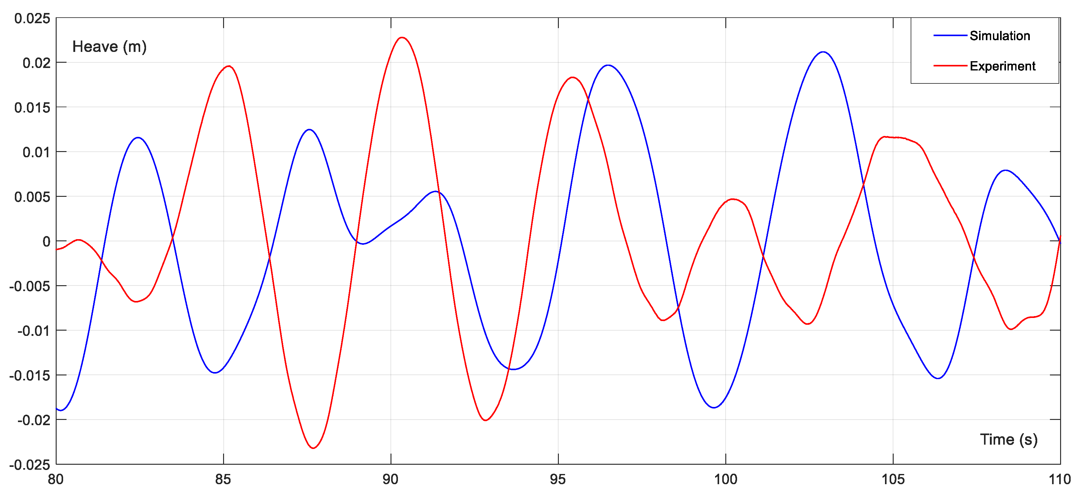
Figure 14.
Example of simulated and measured heave motion at Fr = 0.4 in head seas.
Figure 14.
Example of simulated and measured heave motion at Fr = 0.4 in head seas.
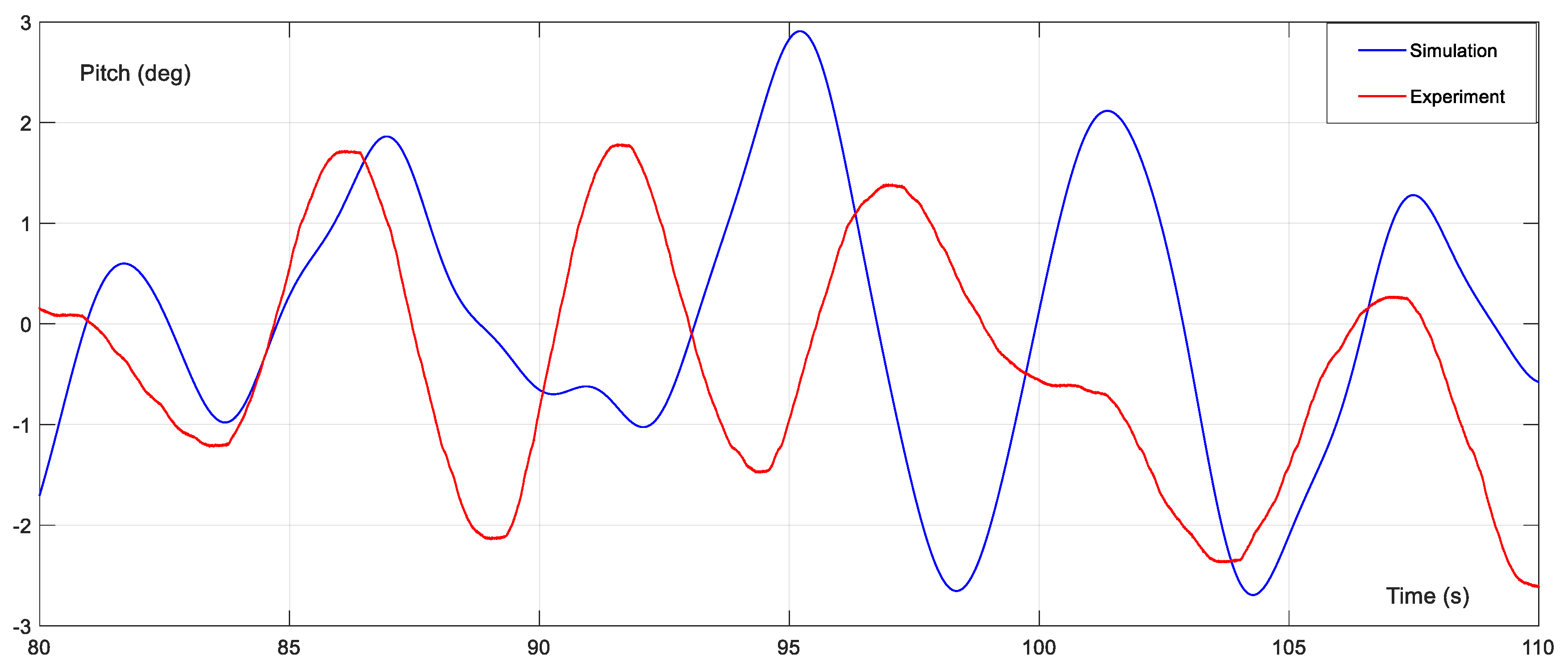
Figure 15.
Example of simulated and measured pitch motion at Fr = 0.4.
Figure 15.
Example of simulated and measured pitch motion at Fr = 0.4.
Figure 16.
Example of simulated and measured cg accelerations at Fr = 0.4 in head seas.
Figure 16.
Example of simulated and measured cg accelerations at Fr = 0.4 in head seas.
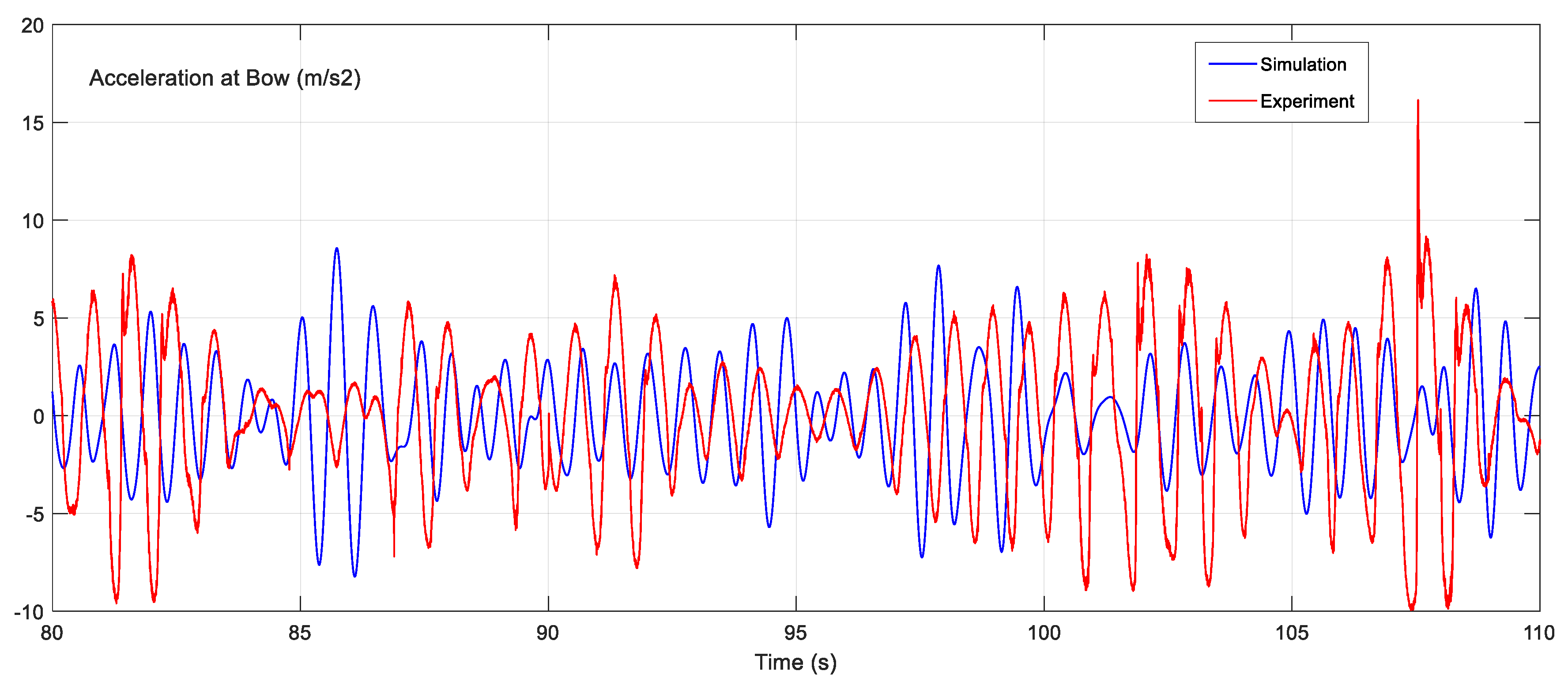
Figure 17.
Example of simulated and measured bow accelerations at Fr = 0.4 in head seas.
Figure 17.
Example of simulated and measured bow accelerations at Fr = 0.4 in head seas.
Figure 18.
Example of simulated and measured heave motion at Fr = 0.4 in following seas.
Figure 18.
Example of simulated and measured heave motion at Fr = 0.4 in following seas.
Figure 19.
Example of simulated and measured pitch motion at Fr = 0.4 in following seas.
Figure 19.
Example of simulated and measured pitch motion at Fr = 0.4 in following seas.
Table 1.
The main characteristics of the tested model.
Table 1.
The main characteristics of the tested model.
| Parameter | Model | Ship |
|---|
| Scale factor λ = 15 | | |
| LOA (m) | 2.000 | 30.000 |
| LWL (m) | 1.994 | 29.910 |
| BWL (m) | 0.494 | 7.410 |
| T (m) | 0.116 | 1.740 |
| ∆ (N,kN) | 342.17 | 1183.7 |
| LCG (m) | 0.932 | 13.980 |
| VCG (m) | 0.204 | 3.060 |
| r55 (kgm2) | 0.487 | 7.300 |
| Static trim (deg) | 0.000 | 0.000 |
| Pos. of the accelerometer at bow (m) (from CoG) | 0.963 | 14.445 |
Table 2.
Wave spectrum characteristics.
Table 2.
Wave spectrum characteristics.
| | SI Unit | Model Scale | Ship Scale |
|---|
| Significant wave height Hs | (m) | 0.096 | 1.44 |
| Peak period Tp | (s) | 1.429 | 5.533 |
| Peakness parameter γ | (-) | 3.3 | 3.3 |
Table 3.
Measured spectra properties-head waves.
Table 3.
Measured spectra properties-head waves.
| | Fr = 0.2 | Fr = 0.4 | Fr = 0.6 |
|---|
| Number of encounters | 144 | 167 | 219 |
| Significant wave height Hs (m) | 0.098 | 0.096 | 0.097 |
| Moment of 0 order (m2) | 0.00060 | 0.00058 | 0.00059 |
| Total Runs Time (s) | 140 | 140 | 140 |
Table 4.
Scaling of hydrodynamic coefficients from Hydrostar® to model scale.
Table 4.
Scaling of hydrodynamic coefficients from Hydrostar® to model scale.
| Parameter | SI | Scale Factor | Model Scale |
|---|
| (kg) | λ3 | 65.185 |
| (kg*m/rad) | λ4 | 9.442 |
| (kg*m) | λ4 | 11.338 |
| (kg*m2/rad) | λ5 | 9.653 |
| (kg/s) | λ2.5 | 91.230 |
| (kg*m/(rad*s)) | λ3.5 | 153.00 |
| (kg*m/s) | λ3.5 | −89.510 |
| (kg*m2/(rad*s2)) | λ4.5 | 23.820 |
| C33 | (kg/s2) | λ2 | 6.356 × 10³ |
| C35 | (kg*m/(rad*s2)) | λ3 | 7.526 × 10² |
| C53 | (kg*m/s2) | λ3 | 7.526 × 10² |
| C55 | (kg*m2/(rad*s2)) | λ4 | 1.258 × 10³ |
Table 5.
Summary of performed experiments and simulations.
Table 5.
Summary of performed experiments and simulations.
| No. | V | β | Fr | TP | fP | ωp | ωEP | Sim Time | Exp Time |
|---|
| | (m/s) | (deg) | (-) | (s) | (Hz) | (rad/s) | (rad/s) | (s) | (s) |
| 1 | 0.879 | 180 | 0.2 | 1.429 | 0.700 | 4.397 | 6.130 | 140 | 140 |
| 2 | 1.758 | 180 | 0.4 | 1.429 | 0.700 | 4.397 | 7.863 | 140 | 140 |
| 3 | 2.635 | 180 | 0.6 | 1.429 | 0.700 | 4.397 | 9.592 | 140 | 140 |
| 4 | 0.879 | 0 | 0.2 | 1.429 | 0.700 | 4.397 | 2.664 | 280 | 230 |
| 5 | 1.758 | 0 | 0.4 | 1.429 | 0.700 | 4.397 | 0.931 | 280 | 224 |
| 6 | 2.635 | 0 | 0.6 | 1.429 | 0.700 | 4.397 | −0.798 | 280 | 191 |
Table 6.
Head seas results comparison.
Table 6.
Head seas results comparison.
| | NUMERICAL_Fr = 0.2 | EXPERIMENTAL_Fr = 0.2 | DIFF (%) |
| | | No. | H1/3 | HMEAN | H1/10 | HMAX | No. | H1/3 | HMEAN | H1/10 | HMAX | HMEAN |
| Heave | (m) | 144 | 0.084 | 0.053 | 0.010 | 0.010 | 118 | 0.065 | 0.060 | 0.119 | 0.170 | −11.4 |
| Pitch | (deg) | 145 | 9.417 | 6.085 | 11.19 | 11.189 | 125 | 9.962 | 6.763 | 13.737 | 17.676 | −10.0 |
| acc_cg | (g) | 137 | 0.383 | 0.262 | 0.441 | 0.441 | 145 | 0.324 | 0.204 | 0.447 | 0.651 | 28.2 |
| acc_bow | (g) | 143 | 0.852 | 0.576 | 0.997 | 0.997 | 148 | 0.875 | 0.556 | 1.158 | 1.521 | 3.4 |
| | NUMERICAL_Fr = 0.4 | EXPERIMENTAL_Fr = 0.4 | DIFF (%) |
| | | No. | H1/3 | HMEAN | H1/10 | HMAX | No. | H1/3 | HMEAN | H1/10 | HMAX | HMEAN |
| Heave | (m) | 170 | 0.102 | 0.071 | 0.123 | 0.123 | 142 | 0.102 | 0.065 | 0.133 | 0.171 | 9.1 |
| Pitch | (deg) | 186 | 8.131 | 5.376 | 10.18 | 10.178 | 149 | 9.535 | 6.236 | 12.008 | 13.747 | −13.8 |
| acc_cg | (g) | 167 | 0.751 | 0.513 | 0.929 | 0.929 | 167 | 0.750 | 0.476 | 1.001 | 1.161 | 7.8 |
| acc_bow | (g) | 173 | 1.305 | 0.8760 | 1.627 | 1.627 | 160 | 1.382 | 0.922 | 1.744 | 2.563 | −5.0 |
| | NUMERICAL_Fr = 0.6 | EXPERIMENTAL_Fr = 0.6 | DIFF (%) |
| | | No. | H1/3 | HMEAN | H1/10 | HMAX | No. | H1/3 | HMEAN | H1/10 | HMAX | HMEAN |
| Heave | (m) | 218 | 0.094 | 0.059 | 0.121 | 0.121 | 173 | 0.083 | 0.055 | 0.110 | 0.132 | 7.3 |
| Pitch | (deg) | 240 | 6.405 | 4.337 | 8.223 | 8.223 | 179 | 5.890 | 3.950 | 7.779 | 9.680 | 9.8 |
| acc_cg | (g) | 219 | 0.897 | 0.612 | 1.173 | 1.173 | 197 | 0.846 | 0.562 | 1.123 | 1.444 | 8.7 |
| acc_bow | (g) | 230 | 1.407 | 0.987 | 1.794 | 1.794 | 191 | 1.261 | 0.834 | 1.727 | 2.568 | 18.3 |
Table 7.
Following seas results comparison.
Table 7.
Following seas results comparison.
| | NUMERICAL_Fr = 0.2 | EXPERIMENTAL_Fr = 0.2 | DIFF (%) |
| | | No. | H1/3 | HMEAN | H1/10 | HMAX | No. | H1/3 | HMEAN | H1/10 | HMAX | HMEAN |
| heave | (m) | 114 | 0.044 | 0.028 | 0.056 | 0.066 | 81 | 0.051 | 0.033 | 0.069 | 0.081 | 14.6 |
| Pitch | (deg) | 117 | 5.688 | 3.602 | 6.730 | 7.722 | 89 | 5.386 | 3.566 | 7.365 | 8.752 | −1.0 |
| acc_cg | (g) | 107 | 0.031 | 0.021 | 0.037 | 0.044 | 70 | | | | | |
| acc_bow | (g) | 102 | 0.059 | 0.041 | 0.069 | 0.077 | 84 | | | | | |
| | NUMERICAL_Fr = 0.4 | EXPERIMENTAL_Fr = 04 | DIFF (%) |
| | | No. | H1/3 | HMEAN | H1/10 | HMAX | No. | H1/3 | HMEAN | H1/10 | HMAX | HMEAN |
| heave | (m) | 50 | 0.037 | 0.024 | 0.043 | 0.049 | 37 | 0.042 | 0.032 | 0.048 | 0.057 | 24.0 |
| pitch | (deg) | 45 | 4.303 | 2.953 | 5.008 | 5.562 | 34 | 4.444 | 3.516 | 4.740 | 4.801 | 16.5 |
| acc_cg | (g) | 75 | 0.005 | 0.004 | 0.007 | 0.009 | | | | | | |
| acc_bow | (g) | 78 | 0.008 | 0.005 | 0.010 | 0.012 | | | | | | |
| | NUMERICAL_Fr = 0.6 | EXPERIMENTAL_Fr = 0.6 | DIFF (%) |
| | | No. | H1/3 | HMEAN | H1/10 | HMAX | No. | H1/3 | HMEAN | H1/10 | HMAX | HMEAN |
| heave | (m) | 120 | 0.049 | 0.034 | 0.059 | 0.068 | 38 | 0.041 | 0.030 | 0.044 | 0.044 | −13.4 |
| pitch | (deg) | 133 | 5.324 | 3.549 | 6.534 | 7.392 | 33 | 4.840 | 3.316 | 5.488 | 6.096 | −7.0 |
| acc_cg | (g) | 213 | 0.050 | 0.033 | 0.060 | 0.074 | | | | | | |
| acc_bow | (g) | 244 | 0.115 | 0.078 | 0.142 | 0.168 | | | | | | |
© 2020 by the authors. Licensee MDPI, Basel, Switzerland. This article is an open access article distributed under the terms and conditions of the Creative Commons Attribution (CC BY) license (http://creativecommons.org/licenses/by/4.0/).

 ,
, 


