IMO Second Generation Intact Stability Criteria: General Overview and Focus on Operational Measures

Abstract

At the beginning of 2020, after a long and demanding process, the Second Generation Intact Stability criteria (SGISc) have been finalized at the 7th session of the International Maritime Organization (IMO) sub-committee on Ship Design and Construction (SDC). At present, SGISc are not mandatory, nevertheless IMO endorses their application in order to assess their consistency and validity. It is envisaged that SGISc can support the design of safer ships, nevertheless such a rules framework might have an impact also on the ship operational aspects in a seaway. In fact, within the SGISc framework, Operational Measures have also been implemented providing guidance and limitations during navigation. After a comprehensive overview about SGISc vulnerability levels and direct stability assessment, this paper provides a specific insight into the methodological approach for the Operational Measures extensively addressed as a complementary action to ship design.

1. Introduction

The so called Second Generation Intact Stability criteria (SGISc) have been finalized during the 7th session of the IMO sub-committee on Ship Design and Construction (SDC) in 2020. Currently, the criteria are intended not to be mandatory but they received the endorsement of IMO, to be extensively applied in the shipping community. It is foreseen that they need further refinement, but it is expected that SGISc will positively influence the ship design process in the next years. The ship stability performance in waves has been addressed by the SGISc, with specific focus on five dynamic phenomena that is, parametric roll, pure loss of stability, dead ship condition, surf-riding and excessive accelerations. An interesting innovation introduced by the SGISc is the multi-layered approach which defines three assessment levels, characterized by different level of accuracy and therefore conservativeness. Adopting this structure, a designer may choose the kind of analysis to be carried out about the ship stability performance.

Moreover, within the SGISc framework, ship operational aspects during navigation have been introduced. It is recognized that, in order to get a safer ship performance, addressing only design aspect cannot be enough. Operational measures should be also taken into account and indications should be provided to the master. For this reason, both Operational Limitations and Operational Guidance have been developed in the SGISc framework.

In the following sections, an overview of the development process that lead to the finalized version of SGISc is given. Moreover, all the five stability failure modes have been presented with a brief description of the vulnerability level requirements. Finally, a focus on the Operational Measures defined by the SGISc is provided with considerations about the relevant approach and the possible acceptable scenarios.

2. From the Intact Stability Code to the Second Generation Intact Stability Criteria

For a long time, through the Rahola criteria [1] and the Weather criterion [2], until the Intact Stability (IS) code issued at the beginning of the 21st Century, the stability of intact ships in calm water has been one of the main topics in the naval architecture field and in the rule making environment. An exhaustive description of the history of intact stability criteria, from the origin up to the IS code, can be found in References [3,4].

During the discussion about the finalization of the IS code, the need to consider more attentively the physics of what may lead to stability failure has been pointed out. This approach, which is less dependant on database of previous incidents, could guarantee criteria in principle applicable regardless the ship typology, adaptable also for new ship projects but above all able to take into account also the dynamic behaviour of ships due to the presence of waves. In the discussion, the new modality has been often named as a physical approach, implying therefore also the possibility to take into consideration the hydrodynamic aspects of a ship in a seaway condition. Adopting such approach requires an enhanced knowledge of the complex behaviour of ship in a rough sea and of the strong non linearities that might entail even the ship capsizing phenomena [5,6,7,8].

The IS code has been finalized in 2008 and the need of performance-based criteria addressing ship stability in a seaway condition has been introduced and highlighted in its text, more precisely within the general provisions of its mandatory part [9] (Part A—Section 1.1).

The stability failure modes identified by the IS code are the ones addressed within the new intact stability criteria [10,11,12] and already previously taken into consideration in some IMO Circulars [13,14]:

• Restoring moment variation due to waves profile (Parametric Rolling and Pure Loss of Stability);
• Stability failure in the Dead Ship condition;
• Manoeuvring-related stability failure (Surf-Riding and Broaching-to).

In the early 2008, during the 51st session of the IMO Sub-committee on Stability and Load lines and on Fishing vessels safety (SLF), an inter-sessional correspondence group was established ad hoc [15] (Section 4.27) with the aim to develop a set of criteria for the above identified stability failure modes. At the 53rd session of SLF in 2010 instead of new generation criteria, it has been proposed the current name of criteria, that is, Second Generation Intact Stability criteria (SGISc). Moreover, the excessive acceleration stability problem was added as a further phenomenon to be addressed in the SGISc framework [16,17]. The framework and the relevant terminology have been identified along with the development of the process for the methodology and the criteria identification. Soon, the task appeared to be complex and the required time for its accomplishment long accordingly.

2.1. The Multi-Layered Approach

The so called multi-layered approach has been an interesting innovation introduced in the SGISc creation. It consists of a set of criteria, defined for each stability failure, characterized by an increasing level of accuracy, in relation with the layer. This approach assumes three assessment levels: the first two levels, namely the vulnerability assessment levels, are meant to identify ships which could be vulnerable to the stability failure under investigation; conversely, the third level is a purely performance-based direct stability assessment. In addition to what above, also the operational aspects of a ship have been considered within the SGISc framework and relevant assessment approaches to identify Operational Measures have been provided as well. The criteria defined at the first vulnerability level (Lv1), for each stability failure mode, are a simplified check to initially separate roughly vulnerable ships from not vulnerable ones. First vulnerability criteria consist of simple assessments, taking into account few ship geometrical data and loading condition parameters, for example, metacentric height and righting moment in calm water. Second vulnerability levels (Lv2) require the knowledge of more details than Lv1; the phenomena are addressed relying on physics-based approaches taking possibly into account the ship dynamic behaviour in a seaway condition. In the criteria of Lv2, the environmental condition are more detailed as well; therefore a wide set of sea states is processed and a sort of long-term analysis is requested to be carried out. The direct stability assessment (DSA) represents the so called third level of the multi-layered approach. It should predict as close as practically possible the actual ship motions in a seaway condition. It should consist of a non-linear time domain numerical simulations considering at least four degrees of freedom and some of their coupling factors. Model tests ensuring the same level of accuracy can be adopted as well. The DSA therefore is the most accurate, but also the most computationally time-consuming level in the SGISc framework. As a supplementary level, the SGISc introduces some measures acting on the environmental conditions and ship operational aspects—such Operational Measure (OM) respectively are named as the Operational Limitations (OL) and Operational Guidance (OG). The latter is a document containing information and recommendation about ship navigation with the aim to reduce the likelihood of failures. Differently, the OL identify restrictions to the ship operability in relation with specific geographical area and environmental conditions, with the aim to avoid stability failures.

The multi-layered structure has been introduced in the SGISc framework with the aim of avoiding unnecessary high computational burden when not necessary, that is, when ships are nor likely to be vulnerable. In the framework, the higher is the level, the more complex is the required analysis. On the other hand, as an inherent consequence, a relevant conservative safety margin is introduced at lower levels. Therefore, the sequential application of levels would be desirable—if a ship is deemed vulnerable by Lv1, the second level criteria should be used in order to understand whether it is really an issue or not; in the case where the ship is also considered vulnerable by Lv2, the DSA should be applied as the last level, as the one characterised by the best possible reliability, before the introduction of operational measures.

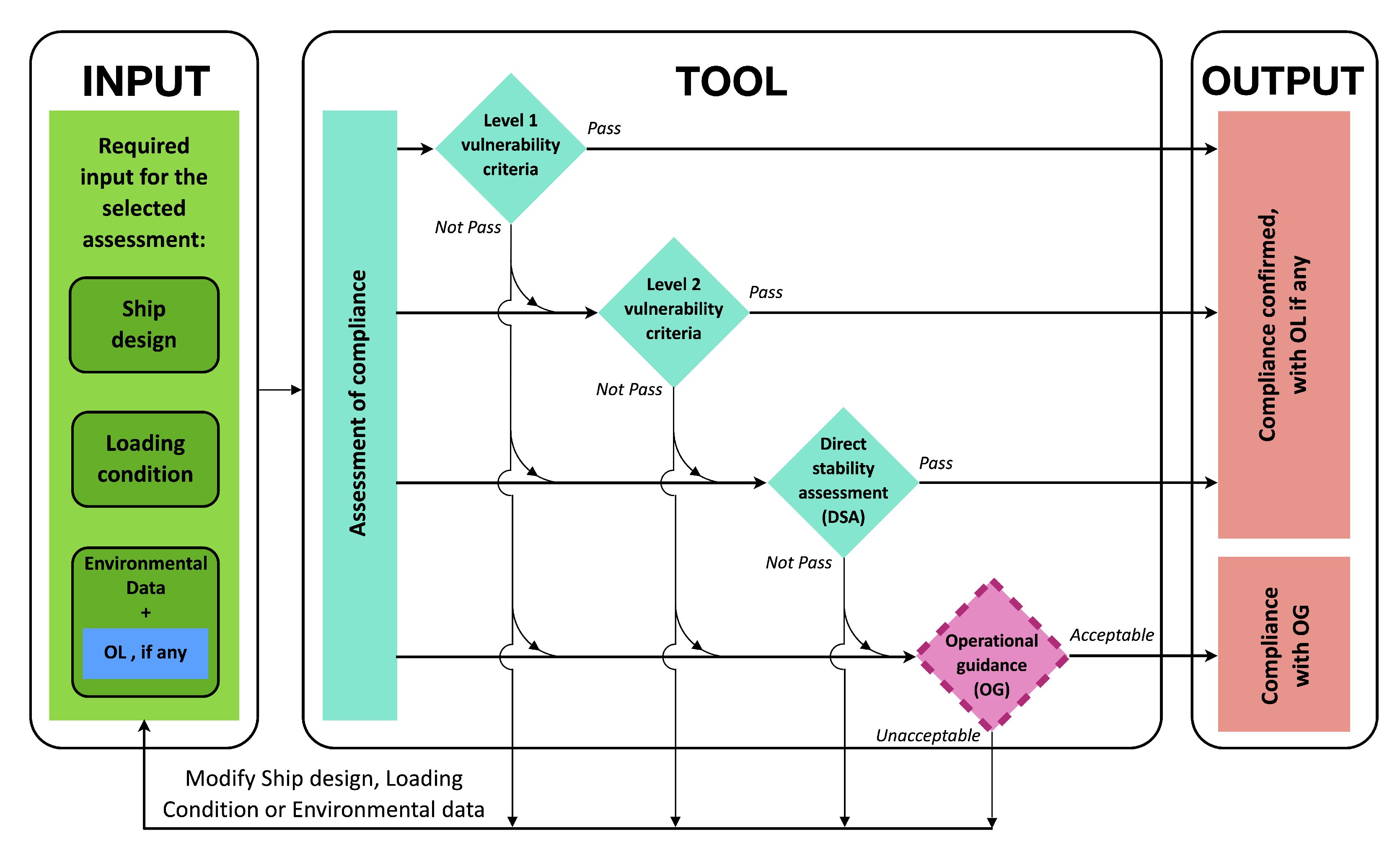
Nevertheless, the finalized version SGISc deem it acceptable that the user can directly apply any design assessment (Lv1, Lv2 or DSA) or operational measures option (OG or OL), without any hierarchy as the one described above. This allow the user to start the design assessment analysis from the DSA or even to directly move to the operational level and apply OL without performing any design assessment. The simplified scheme of the application logic of SGISc is given in Figure 1.

Applying the multilayered approach in a sequential logic (from Lv1 to DSA), it is expected that the higher level gives a more reliable answer in confirming the vulnerability of the ship or in rejecting it. On the contrary, a consistency problem between levels can be identified when a lower level considers the ship not vulnerable while a higher level deems the opposite. In this perspective, during the development of the different criteria for the various vulnerability assessments, concerns about consistency of results rose, especially when Lv1 and Lv2 criteria are compared [18,19,20,21]. Most of the issues have been fixed during the refinement of the criteria formulation, even if some consistency problem still remains. In this perspective, failure modes have different evidences, for example, Lv1 and Lv2 for dead ship condition may provide non consistent results or Lv2 for pure loss of stability may appear too much conservative for ship with low freeboard. In order to bypass these consistency issues, the sequential application of the multilayered approach is not binding and the user can take advantage of the criteria support in the way it is deemed as the most appropriate.

2.2. Toward the Finalization

The SGISc development process has been articulated along the years thanks to the intense work of the inter-sessional correspondence groups and the activity during the sessions of the IMO Sub-Committees in charge (the SDC replaced the SLF after 2013). About four years since the beginning of SGISc development, the first structured draft text of the criteria has been presented at IMO [22] (Annex 1 and Annex 2). Meanwhile, a draft text also of explanatory notes has been drawn up, gathering relevant information about the physics background of each stability failure mode and the criteria formulation [23] (Annex 1–5). After this first milestone, the working group proceeded to develop the guidelines identifying the fundamental features of the numerical tool required for an appropriate DSA. The Sub Committee instructed the correspondence group to develop the DSA procedures separately for each stability failure. The first version of the Guidelines for Direct Stability Assessment have been presented at the 1st SDC session in 2014 [24] (Annex 27). Between the 5th and 6th session of SDC, the consolidated version of the vulnerability level criteria has been finalized as well as the DSA guidelines. Also the Operational Measures has been put in the final form in the same very intense period by the inter-sessional correspondence group. Eventually, as an epochal moment, the final version of the Guidelines on the second generation intact stability criteria has been adopted at the 7th session of SDC [25]. A further step still needed is to complete the explanatory notes; this activity is intended to be carried out within the next SDC sessions.

The SGISc have been issued as a complementary analysis aside the mandatory criteria defined in the part A of IS code. The Guidelines will be kept under review for a trial period during which the stakeholders are encouraged to provide feedback on SGISc application on existent and new ships. In the Guidelines is clearly stated that SGISc are not intended to be used instead of the existing mandatory criteria.

3. Details about Design Assessment

As stated above, SGISc address pure loss of stability (PLS), parametric rolling (PR), surf-riding (SR), dead ship condition (DS) and excessive accelerations (EA). In this section, a brief description of the physics behind each phenomenon and the requirements of each criterion is given. The final version of vulnerability levels and DSA for SGISc, as approved at 7th session of SDC, can be found in Reference [25] (Chapters 2–3).

3.1. Restoring Arm Variation Due to Waves

This phenomenon is related to the interaction between the hull geometry and the encountered wave profile. When a longitudinal wave having a length comparable to the ship length encounters a vessel, variations of waterplane area and immersed volume distribution are registered. This has an effect on the ship restoring capability. The worst case happens when the wave crest is located amidships entailing a righting arm decrease that, in comparison with the one in calm water, can be quite critical. The opposite happens when the wave trough is amidships: in this case the effect is a strengthening of the righting moment.

This phenomenon may lead to two different stability failures, that is, pure loss stability and parametric rolling. The typical scenario, that better characterizes PLS, considers a longitudinal wave as long as the vessel, approaching from stern with a celerity just faster than the ship speed. In this situation, the wave takes a long time to pass the vessel and the critical situation, with the wave crest amidship, lasts considerably decreasing the stability performance for a not negligible time.

PR can happen when the ship interacts with a train of waves having the length comparable to the ship length and an encounter period that is half of the ship natural roll period. The typical scenario for PR can be depicted as follows: when the ship is far away from its upright position and the wave trough is amidships, the righting arm is “stronger” and therefore the ship is vigorously pushed back to the upright position. When the ship is in the upright position, the wave crest has already moved amidship. In this condition, the righting moment is “weaker” and the ship rolls to an even larger heel angle on the opposite side. If the wave trough moves again amidships when the maximum heel angle on the opposite side is reached, the cycle starts again leading to heel angles larger and larger.

3.1.1. First Vulnerability Levels for PLS and PR

First levels for PLS and PR assess the metacentric height variation due to the wave profile with a very simplified formulation. Both the levels evaluate an upright hydrostatics at the draft of the specific wave trough. PR requires also an additional hydrostatics at the draft of the wave crest of the same specific wave. The wave characteristics are a length equal to the ship length and a steepness factor of $S_W=0.0334(-)$ for PLS and $S_W=0.0167(-)$ for PR.

The assessed loading condition of a ship is not judged vulnerable to PLS when condition (1) is verified.

$$G{M}_{min}\ge 0.05\left(\mathrm{m}\right),$$

(1)

where $G{M}_{min}$ is the metacentric height calculated for the hydrostatics at the drafts defined above.

The assessed loading condition of a ship is not judged vulnerable to PR when condition (2) is verified.

$$\frac{\Delta G{M}_1}{GM}\le R_{PR},$$

(2)

where $GM$ is the metacentric height in calm water for the considered loading condition; $\Delta G{M}_1$ is defined as $\frac{I_{T_H}-I_{T_L}}{2·\nabla }$; ∇ is the immersed volume; $I_{T_H}$ and $I_{T_L}$ are the transverse moment of inertia of the waterplane located respectively at the drafts corresponding to the wave crest and the wave trough. The standard $R_{PR}$ is defined as a function of breadth, length, amidship coefficient and the bilge keel projected area; it ranges from 0.17 (−) to 1.87 (−).

Moreover, both criteria consider a ship vulnerable if the condition (3) is not verified.

$$\frac{{\nabla }_D-\nabla }{A_W·(D-d)}\ge 1.0.$$

(3)

3.1.2. Second Vulnerability Levels for PLS and PR

The structure of second vulnerability levels is very similar among all the stability failure modes addressed within the SGISc framework. A sort of long-term analysis is undertaken, based on the wave scatter diagram of North-Atlantic ocean, as shown in Equation (4). This analysis implies at first a short-term assessment for each sea state, which is different for the various stability failure modes.

$$C=\sum _{H_S}\sum _{T_Z}{C}_S·W(H_S;T_Z).$$

(4)

Second vulnerability level for PLS judges a ship not vulnerable if condition (5) is verified.

$$max\left(C{R}_1;C{R}_2\right)\le R_{PL0},$$

(5)

where $R_{PL0}=0.06(-)$; $C{R}_1$ and $C{R}_2$ are the long-term indexes evaluating respectively the capsizing angle in waves and the static equilibrium heel angle under the action of a heeling lever $l_{PL2}$ considering the restoring moment in waves. The wave to be considered are obtained by filtering the wave scatter diagram by means of the Grim’s wave theory [26,27].

Second vulnerability level for PR considers a ship not vulnerable if condition (6) is verified.

$$C1\le R_{PR1}\hspace{1em}\mathrm{or}\hspace{1em}C2\le R_{PR2},$$

(6)

where $R_{PR1}=0.06(-)$; $R_{PR2}=0.025(-)$; $C1$ and $C2$ are the long-term indexes. The first long-term index takes into account the actual GM variation in waves evaluated for 16 different waves defined within the criterion. The long-term index $C2$ needs a 1-DoF model able to reproduce roll motions when the ship interacts with longitudinal waves. The waves required by the latter analysis are obtained as specified in the second level criteria for PLS.

3.2. Manoeuvring-Related Stability Failure

Manoeuvring-related stability problems are those referring to the broaching-to and surf-riding stability failure modes. These phenomena are strictly linked, in fact, broaching is preceded by surf-riding as studied in References [28,29].

Broaching-to can be defined as a sudden and uncontrollable turning despite the opposite action of the rudder to counter act it. This phenomenon may lead to large heel angle and even the capsizing. Instead, the surf-riding happens when a quartering waves with specific characteristics reaches the vessel and accelerates it at the wave celerity. In this condition most of the ships are directionally unstable, thus broaching-to may occur. In light of this relation between broaching and surf-riding, the developed criterion assess ship vulnerability to the latter in order to prevent broaching-to.

Surf-riding phenomenon may develop when the ship speed is comparable to the wave celerity and the wave length is about one to three times the ship length, together with a wave steepness great enough to generate a sufficient wave surge force. Surf-riding is characterized by two ship speed thresholds. A ship is affected by the surge motion when the speed is below the first threshold and SR cannot happen. In this condition, a vessel is accelerated by the front part of the approaching wave and then it is decelerated by the back part of the passing wave. Over the first speed threshold surf-riding may occur only under a specific condition. This condition depends mainly on the relative position between the ship and the wave crest. Finally, when the ship speed overreaches the second threshold, SR occurs under any condition. Due to the relative high speed of the vessel, the wave having the above mentioned characteristics trigger the surf-riding regardless the relative position between the ship and the wave crest.

3.2.1. First Vulnerability Level for SR

First vulnerability levels for SR is made up of a very simple assessment. A ship is judged not vulnerable if relations (7) are verified.

$$L\ge 200\left(\mathrm{m}\right)\hspace{1em}\mathrm{or}\hspace{1em}\mathrm{Fn}\le 0.30(-),$$

(7)

where L is the ship length and $Fn$ is the Froude number at the service speed.

3.2.2. Second Vulnerability Level for SR

The second vulnerability level for SR adopts the same structure defined in condition (4) as a long-term assessment. A ship is judged not vulnerable to SR if condition (8) is verified.

$$C\le R_{SR},$$

(8)

with $R_{SR}=0.005(-)$.

For this stability failure mode the short-term index is evaluated as defined in Equation (9).

$$C_S(H_S;T_Z)=\sum _{i=0}^{N_{\lambda }}\sum _{j=0}^{N_a}{w}_{ij}·C{2}_{ij},$$

(9)

where $w_{i,j}$ is a statistical weighting factor calculated with the joint distribution of local wave steepness and lengths; $C{2}_{i,j}$ is a coefficient as a function of the critical Froude number and the service ship speed. The coefficient $C2$ is evaluated by an iterative procedure where the equilibrium among ship resistance, propeller thrust and wave surge are pursued.

3.3. Dead Ship Condition

The stability problem related to the dead ship condition is already addresses by the so called weather criterion included in the IS code. Moreover, the MSC.1 Circular 1200 [30] has been issued by IMO during the IS code revision, introducing alternative assessment procedure for the weather criterion. All the same, it has been decided to address this stability failure mode in the SGISc framework adopting a more precise physical-based analysis.

The typical scenario of DS considers a ship which has lost its power and it is rolling under the action of wind and waves, usually turned in beam seas. The ship is assumed to be inclined leeward while rolling under the combined effect of wind and waves. In this situation, a sudden wind gust acts on the vessel when it is at the maximum windward roll angle. The criterion is aimed to assess the acceptable value of the dynamic angle of equilibrium under this circumstances.

3.3.1. First Vulnerability Level for DS

First vulnerability criterion for DS embeds the Severe wind and rolling criterion known as the weather criterion and defined in Reference [9] (Chapter 2). It differs only for the table of wave steepness factor, which is replaced by the extend version introduced in Reference [30]. The weather criterion is an energy-based model where the energy balance between the wind action and the righting moments is assessed.

3.3.2. Second Vulnerability Level for DS

The second vulnerability level for DS adopts a different approach with respect to the first level. Often, this is the origin of some inconsistency issues between the two levels. The Lv2 criterion relies on a dynamic-based method where the environmental condition and the ship characteristic parameters are modelled by means of a 1-DoF computational tool. This kind of analysis has to be carried out for each sea state defined in the wave scatter diagram. As a result of this dynamic assessment a short-term index is obtained.

Also in this case, a long-term analysis is carried out according to condition (4). A ship is judged not vulnerable if condition (10) is verified.

$$C\le R_{DS0},$$

(10)

where C is the long-term index and $R_{DS}=0.06(-)$ is the standard threshold.

3.4. Excessive Acceleration

The EA stability failure mode has been introduced in the SGISc assessments after a list of casualties had been submitted to IMO consideration. In particular, this problem usually involves vessels sailing in ballast condition having high values of metacentric height.

The scenario considered in the formulation of EA criteria entails the ship rolling under the action of pure beam seas in the zero-speed condition. Looking at a selected point located on board, the higher is the vertical distance from the roll axis, the longer is the shift to be covered in a half roll period. Since the angular roll velocity is constant along the whole ship, the highest point has the fastest linear velocity in order to cover in the same time a longer distance. Since every half roll period the roll motion changes its direction, also the linear velocity direction changes and this leads to a linear transverse acceleration. The faster is the linear velocity change, the larger is the transverse acceleration due to roll motion. With reference to the close relationship between the roll period and the metacentric height, if the latter is higher the roll period is shorter and in turns this implies that large transverse acceleration may occur during roll motion.

Transverse acceleration is very dangerous onboard, both for the cargo and the crew members. Beside seasickness, it may cause loss of balance, fall or even being thrown against bulkheads or furniture. The same for the cargo, which may fall outboard or get damaged.

3.4.1. First Vulnerability Level for EA

A ship is judged not vulnerable to EA according to Lv1 if condition (11) is verified.

$$\phi ·k_L·\left(g+4{\pi }^2·\frac{h_r}{T_{roll}^2}\right)\le R_{EA1},$$

(11)

where $R_{EA1}=4.64(\mathrm{m}/{\mathrm{s}}^2)$ is the standard; $\phi$ is the characteristic roll amplitude; $k_L$ is a coefficient taking into account simultaneous action of roll, yaw and pitch motions; g is the gravity acceleration; $T_{roll}$ is the roll period and $h_r$ is the vertical distance between the roll axis and the highest point where crew or passenger may be present.

3.4.2. Second Vulnerability Level for EA

The second vulnerability level for EA requires to perform a long-term analysis as defined in condition (4). The short-term index to be considered is given in Equation (12).

$$C_S=exp\left(-\frac{R_2^2}{2{\sigma }_{LA}^2}\right),$$

(12)

where $R_2=9.81(\mathrm{m}/{\mathrm{s}}^2)$ and ${\sigma }_{LA}$ is the standard deviation of the lateral accelerations at zero speed in a beam sea. The short-term index $C_S$ represents the probability to exceed a specified lateral acceleration.

3.5. Direct Stability Assessment: Requirements & Methodology

The DSA can be considered the third level of assessment and it represents the most reliable approach able to evaluate ship stability performances in a seaway condition. Nevertheless, due to the complexity of the investigated phenomenon (i.e., dynamic behaviour of a ship in a seaway), its satisfactory formulation and implementation is challenging. To this regard, significant steps forward have been made in latest years, with promising results [31,32].

The DSA has been conceived to enable the measurement of the level of safety in terms of average stability failure rate, namely the probability that the stability failure event may occur over a specified period of time. As concern the SGISc framework, the failure event is defined as either the exceedance of roll angle or the exceedance of lateral acceleration. The former is defined as the minimum value among 40${}^{°}$, the capsizing angle or the downfloading angle, all evaluated in calm water. The considered acceleration should be evaluated at the highest point on board the ship where crew members and/or passengers may be present, the threshold should be compliant with 9.81 (m/s${}^2$).

The procedure for the DSA can be split in two main parts: the methodology able to reproduce reliable ship motions in a seaway, even at very large heel angles, and the post-processing procedure. Detailed specifications and requirements about DSA can be found in the Guidelines for direct stability assessment [25] (Chapter 3).

3.5.1. Prediction of Ship Motions

The method to adequately model and predict ship motions can be done either by a numerical tool, a model test or a combination of them. Whichever is the selected method, it should be able to reproduce the ship motions in irregular seas. Depending on the investigated stability failure, the direct assessment tool should replicate identified degrees of freedom in the time domain simulation, considering coupling factors among motions. In

Table 1. Degrees of freedom required in the simulation of particular stability failure modes.

Stability Failure Mode	Surge	Sway	Heave	Roll	Pitch	Yaw	General Note
Dead Ship Condition	-	X	X	X	X	-	Aerodynamical forces should be taken into account.
Excessive Acceleration	-	-	X	X	X	-	When sway motion is not modelled, care about lateral acceleration reproduction should be paid.
Parametric Rolling	-	-	X	X	X	-	-
Pure Loss of Stability	X	X	-	X	-	X	-
Surf-Riding/Broaching-to	X	X	-	X	-	X	Hydrodynamical forces due to vortex shedding should be properly modeled.

For those degrees of freedom not included in the dynamic modelling, static equilibrium should be assumed.

, required degrees of freedom to be modelled during the simulation for each stability failure mode are given.

In the guidelines, the requirements for the numerical tools are defined as well as how to model the roll damping coefficient, forces and moments acting on the hull. In order to comply with the necessary qualitative and quantitative validations, the numerical tool could be calibrated by means of model tests. The qualitative validation should ensure that the numerical tool is able to reproduce the physics of the stability failure mode considered. The quantitative validation should ensure the degree of accuracy the software is capable to reproduce the stability failure mode. As concern the prediction of ship motions, it is worth mentioning that it is sufficient to be validated only for the phenomenon considered. Therefore, the validation of numerical tool is failure-mode specific.

3.5.2. Post-Processing of Results

Within the so called post-processing procedure, the estimation of the likelihood that a stability failure may occur is to be calculated. The Guidelines for DSA define three different approaches for such activity:

• Full probabilistic assessment;
• Probabilistic criteria for assumed design situation; and
• Deterministic criteria for assumed design situation.

The first method reproduces as accurately as possible the actual ship operative life, considering every combination of sea states, ship speeds and headings. The criterion is the estimate of the mean long-term stability failure rate, which is calculated as the average over all the combinations that have been simulated. All the stability failures, except for DS, should be simulated considering the heading ranging uniformly from 0${}^{°}$ to 180${}^{°}$ as well as the ship forward speed should be distributed from zero to the maximum speed. For the DS stability failure, simulations should be carried out considering beam seas and zero speed condition. Since stability failures may be rare, the full probabilistic method requires additional effort in the solution of the problem of rarity, especially when the mean time to failure is very long with respect to the ship natural roll period. In order to circumvent this issue, methods relying on a selection of assumed design situations have been introduced.

The assumed design situations are specifically defined for each stability failure mode, addressing the wave directions, ship speeds and wave periods to be considered in the simulation. Introducing these constrains, the amount of simulations and their duration is notably decreased. The assumed design situation can be assessed with either probabilistic or deterministic criteria. The probabilistic criteria takes into account the maximum stability failure rate over all the simulations for the considered failure mode. To reduce further the simulation time, the deterministic criterion takes into account the greatest mean three-hour maximum roll amplitude or lateral acceleration. Because of the large level of inaccuracy introduced by the deterministic procedure, an additional margin has been added in the selection of the standard: the thresholds have been halved.

In addition to the specifications and requirements for the assessment procedures described above, in Reference [25] (Chapter 3) judging criteria are reported as well, to verify whether the failure recorded during a simulation can be considered as the failure mode for which the numerical tool is validated. Since the validation of the numerical tool or model test procedure is failure-mode specific, for each phenomenon a set of different criteria is provided in the Guidelines for DSA.

4. An Overview on the Operational Measures

It is recognised that safety cannot only be a matter of ship design. To enhance the level of safety of a vessel in a seaway condition, an approach complementary to the ship design is required, as is also recognised in References [33,34]. This can be implemented with operational measures provided to the master, suggesting the safest behaviour in handling ship navigation for specific environmental conditions. It is worth pointing out that, however, when a vessel or a specific loading condition are affected by too many operational restrictions, it means that a refinement of the ship design is needed. Considering the framework of SGISc, the OM have been categorized in two typology—Operational Limitations and Operational Guidance.

4.1. Operational Limitations

Operational Limitations define operational limits to the navigation, for a specific loading condition, delimiting the environmental condition. The environmental condition may be limited by the OL with two restriction typologies. The first typology is related to the geographical areas where the ship sails (i.e., sheltered water, specific sea area and route) or it can be a seasonal limitation when the likelihood of stability failure is higher. This kind of limitation is called in the IMO document as Operational limitations related to areas or routes and season. The second OL typology is related to the significant wave height that the vessel is able to safely cope with during navigation. It is named Operational Limitations related to maximum significant wave height by IMO document.

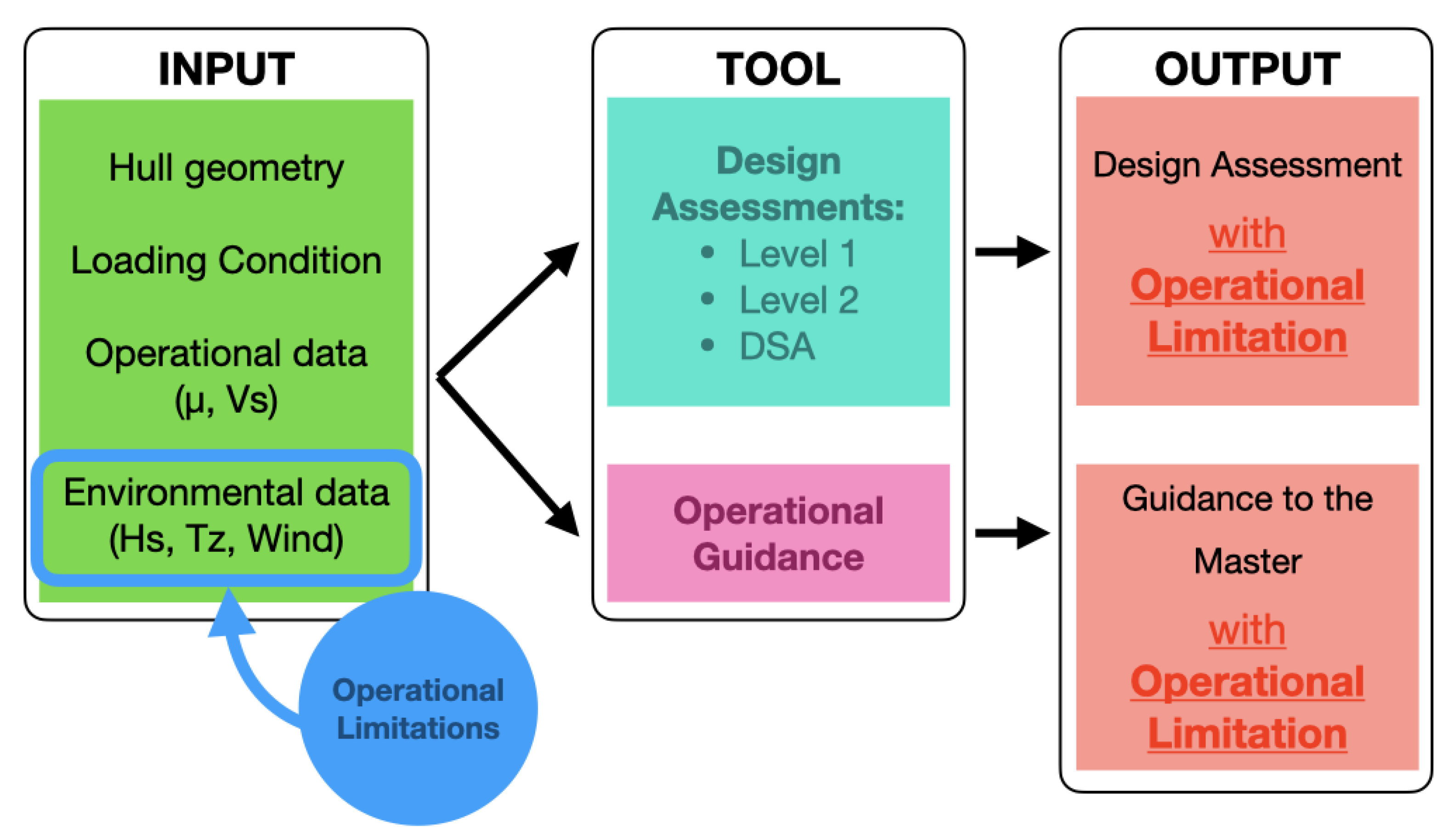
OL need an assessment tool in order to be identified, for example, vulnerability levels or direct stability assessment. For this reason, OL may be considered a tool able to tune the considered operational profile in the design assessment. This concept is facilitated by the modularity structure of the SGISc which are formulated to easily introduce modifications to selected methodologies or boundary conditions. Therefore, OL should be considered as a complementary instrument to the assessment process and not as a stand-alone assessment tool. A graphical representation of this concept is proposed on Figure 2.

In the SGISc, the environmental conditions can be modified by directly acting on the wave scatter diagram which is considered for the evaluation of the long term stability failure rate for each phenomena. Possible restrictions are aimed to reduce at an acceptable level the risk that a stability failure event occurs in a seaway. As regards the OL related to the geographical area, the whole scatter diagram is replaced accordingly, thus, real time weather forecasts are not required for this restrictions. On the contrary, OL related to the significant wave height modify the wave scatter diagram cutting-off sea states having a significant wave height greater than the selected threshold. The obtained scatter table is named limited scatter table. This limitation implies that detailed weather forecast, including significant wave heights, must be available to the master in real time, in order to avoid the limited sea states. Interesting applications of OL have been presented in References [35,36].

4.2. Operational Guidance

The Operational Guidance defines all the situations that are not recommended or should be avoided for each sea state during the navigation. An assumed situation represents the combination of ship operational parameters, such as ship speed and wave encounter heading (i.e., sailing condition) together with the environmental characteristics, that is, significant wave height, zero-crossing wave period, wind direction and gust characteristics. OG defines a set of operative information that support the master in the ship navigation for determined sea states. Following the suggestions of OG, the rate of a stability failure is decreased to an acceptable level. Since the OG is drawn up during the design phase, it is important that guidance addresses all the possible sea states the ship might encounter in relation with the area of navigation. As required for the OL related to the wave height, OG can be fully used only if weather forecast are available on board. In particular, detailed sea state information are beneficial for the master to plan the safest sailing condition (i.e., ship speed and heading) according to the OG.

In the SGISc framework, three different approaches have been defined in order to prepare the OG for each loading condition. They differ for the methodology which predicts the stability failure rate. According to their accuracy, an appropriately conservative threshold is introduced in order to guarantee the same level of safety. The three OG approaches are the following:

• Probabilistic operational guidance;
• Deterministic operational guidance;
• Simplified operational guidance.

The simplified OG are based on simple methodologies such as those introduced in the vulnerability levels. The other two approaches share the same method adopted in DSA, that is, a model test or a numerical calculation tool able to reproduce ship motions in the time domain with at least three degrees of freedom, considering coupling factors and necessary non linearities in irregular seas. More precise technical requirements for these methodologies are given in Reference [25] (Chapter 4).

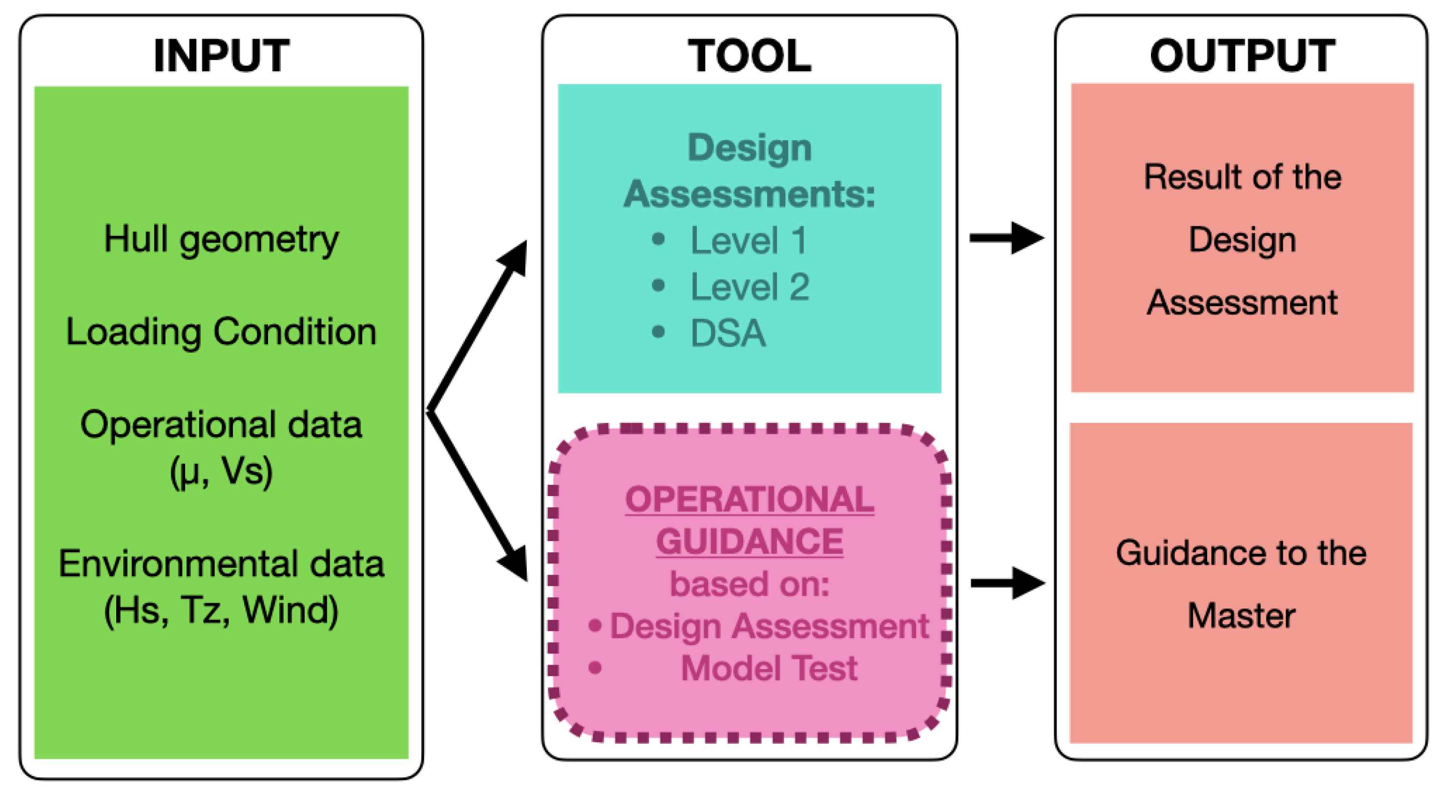
As a consequence of the requirements briefly described above, OG can be considered an additional assessment level independent from the design assessment (i.e. Lv1, Lv2 and DSA). Although it may share the same methodology, OG can be directly performed without assessing the ship vulnerability for a specific stability failure with another assessment tool. This concept is schematically represented in Figure 3.

4.3. Acceptance of Operational Measures

Because of their different concept, OG and OL can be combined together with a multiple choice of combinations. The number of possible cases increases even more when also the design assessments are taken into account. Therefore, a single loading condition can be deemed acceptable according to a set of options defined in Reference [25] (Section 4.4). These configurations have been enumerated below and gathered in Figure 4.

• Acceptable for unrestricted operation. This case is applicable when the design assessments have been satisfied for each stability failure mode. Thus, no OG or OL are provided for the considered loading condition.
• Acceptable for limited operation. In this case, the design assessment of one or more stability failure modes have been passed with operational limitations (e.g., limitations on wave height or on geographical area), while the remaining stability failure have been accepted with unrestricted operation, that is, without any kind of restrictions.
• Acceptable for operation using onboard operational guidance. In this configuration, the loading condition is deemed acceptable if operational guidance are provided without any restrictions for one or more stability failure, and the remaining stability failure satisfy the design assessment either with unrestricted or limited operation.
• Acceptable for operation in a specified area or in a specified route during a specified season. This configuration is achieved when the design assessment for one or more stability failure mode has operational limitations related to areas or routes and season. The remaining stability failure modes do not evidence any vulnerability during the design assessment for unrestricted operation.
• Acceptable for limited operation in a specified area or in a specified route during a specified season. This option allows the loading condition to have an operational limitation related to the significant wave height in a specific area or route and season for one or more stability failure modes. The remaining stability failure mode can be satisfied either with operational limitation related to the area or route and season (i.e., no limitations on the wave height) or without any other restriction nor guidance.
• Acceptable for operation using onboard operational guidance in a specified area or in a specified route during a specified season. In this configuration, the loading condition is judged acceptable if operational guidance are provided together with limitations related to the area or route and season for one or more stability failure modes. The remaining stability failure can be provided either with operational limitations for the same area or route and season, otherwise without any restrictions on the design assessments.

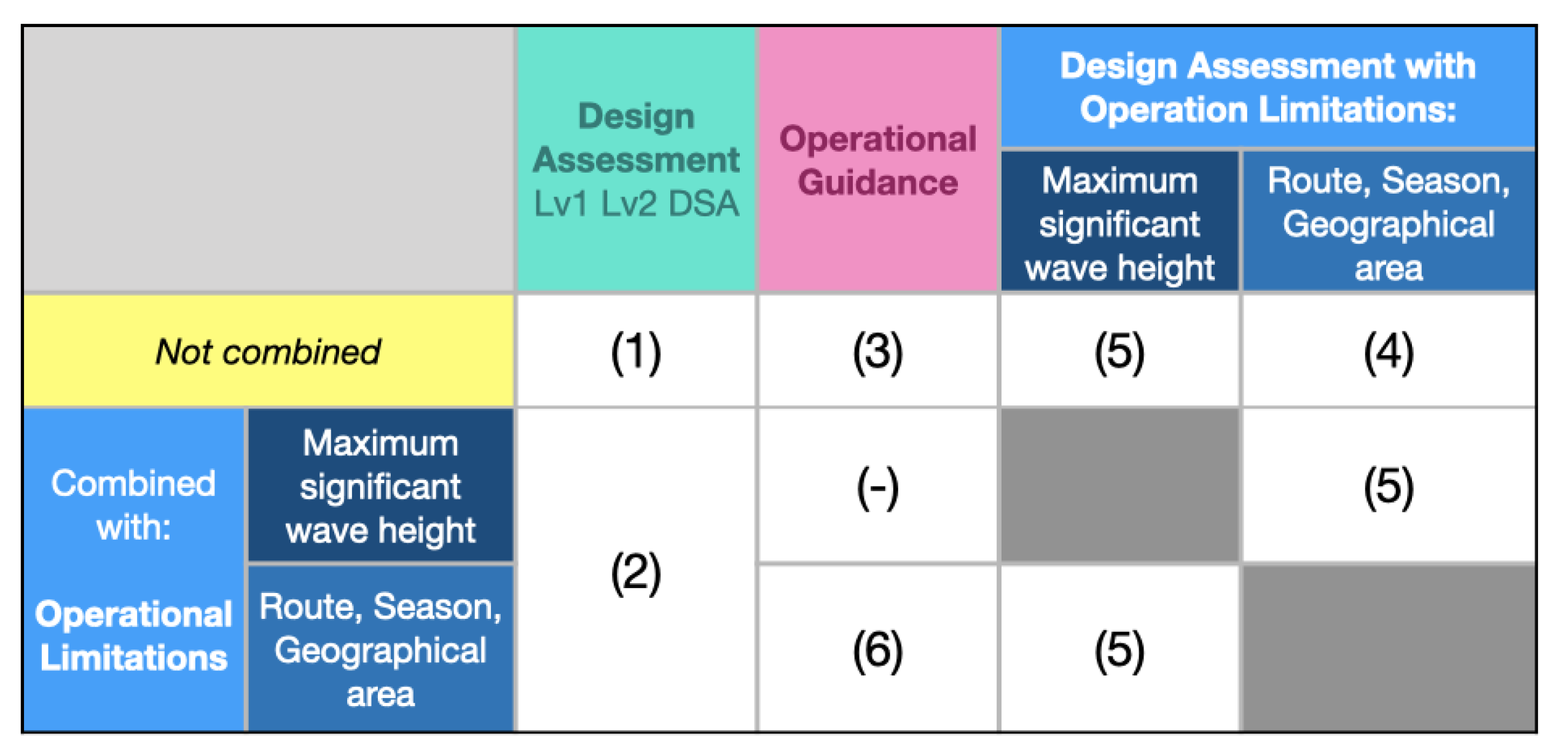
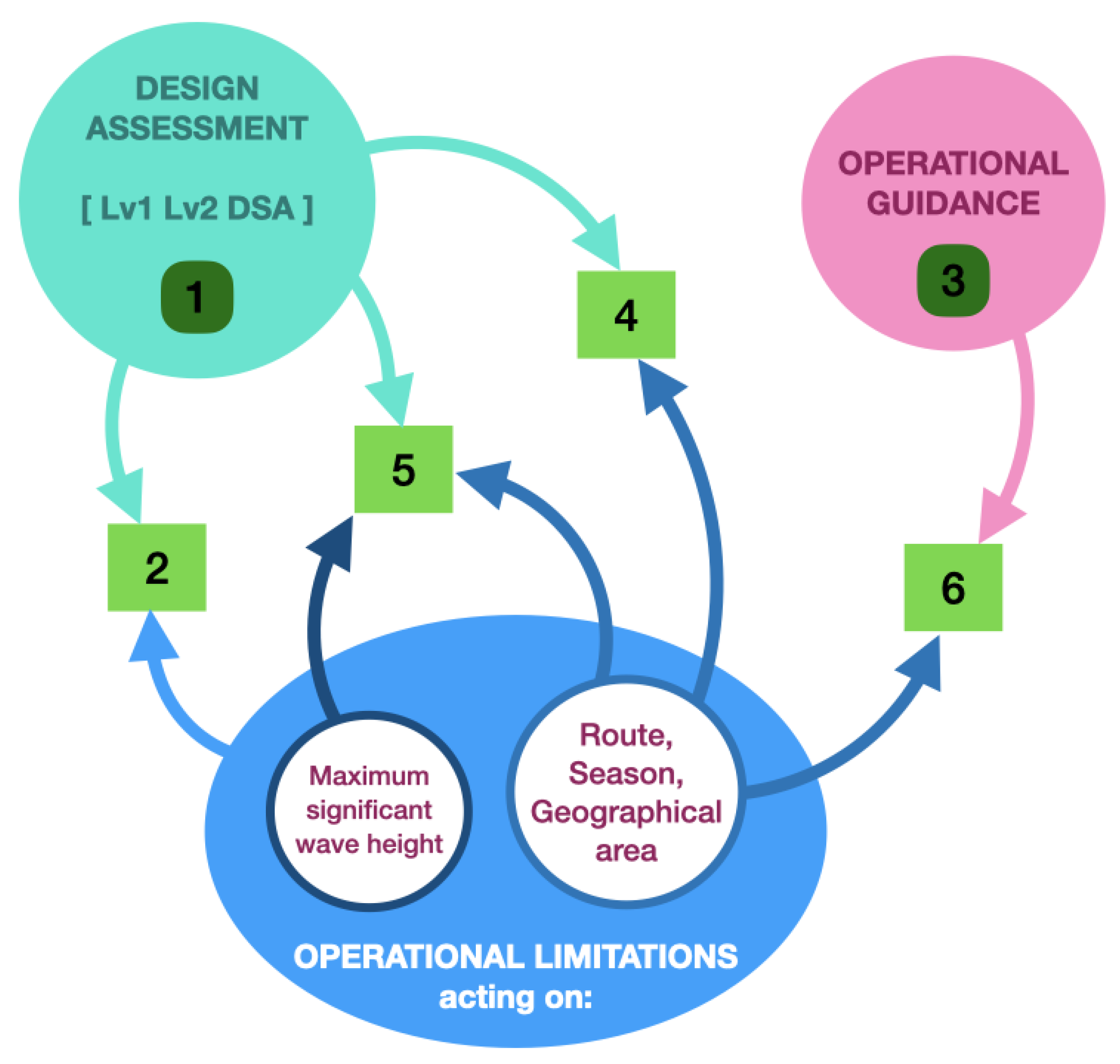
A schematic representation of all possible cases is proposed in Figure 5. Design assessment made up of vulnerability levels (Lv1 and Lv2) and the DSA is represented. The OG and the OL are evidenced as well. The latter is divided in two sub-domains making reference to the two typologies of limitations (i.e., those related to the significant wave height and to a specific area or route and season). The number in the square stands for the possible configuration, while the arrows indicate which tools are combined in it (i.e., design assessment, operational limitation or operational guidance). Looking at the graph, it is possible to point out that only design assessment and OG may exist alone (configuration 1 and 3) while this is not true for the OL.

It is important to highlight that operational guidance may indicate as safe some sailing conditions in relation to the roll motion disregarding other technical aspects, for example, limits of propulsion and steering systems, excessive vertical loads as well as slamming. This should be taken into account in order to avoid misleading OG that can jeopardise vessel navigation because of other problems. For example, sometimes transverse excessive accelerations can be reduced with increasing forward ship, but high speeds cannot be reached in some sea states or may lead to larger vertical motions and slamming.

5. An Example of Application and Results

In order to appreciate the effectiveness of vulnerability levels and operational limitations, an application to a representative Ro-Ro pax ferry is given in this section. In particular, pure loss of stability, dead ship condition and excessive acceleration have been analysed.

Principal vessel dimensions are shown in

Table 2. Ro-Ro pax ferry main dimensions.

Main Dimensions
Length overall	L${}_{\mathrm{OA}}$	211.20	(m);
Length according IS code	L${}_{\mathrm{ISc}}$	200.55	(m);
Maximum breadth	B${}_{\max }$	30.40	(m);
Design draught	d	7.82	(m);
Displacement	$\Delta$	28,234	(t);
Service speed	V${}_{\mathrm{S}}$	22.0	(kt);
Block coefficient	C${}_{\mathrm{B}}$	0.650	( - );
Bilge keel length	L${}_{\mathrm{BK}}$	66.0	(m);
Bilge keel span	b${}_{\mathrm{BK}}$	0.30	(m);
Design vertical centre of gravity	KG	13.43	(m);
Design metacentric height	GM${}_{\mathrm{design}}$	1.43	(m).

. In this analysis four drafts have been considered as representative of the most common loading conditions, that is, Departure and Arrival condition considering loaded on board only trucks or only cars. For the EA assessment, the highest point where people may be present is located in x = 169.8 (m) and z = 34.0 (m). For the DS assessment, the considered lateral exposed surface is about A${}_{\mathrm{L}}$ = 5400 (m${}^2$).

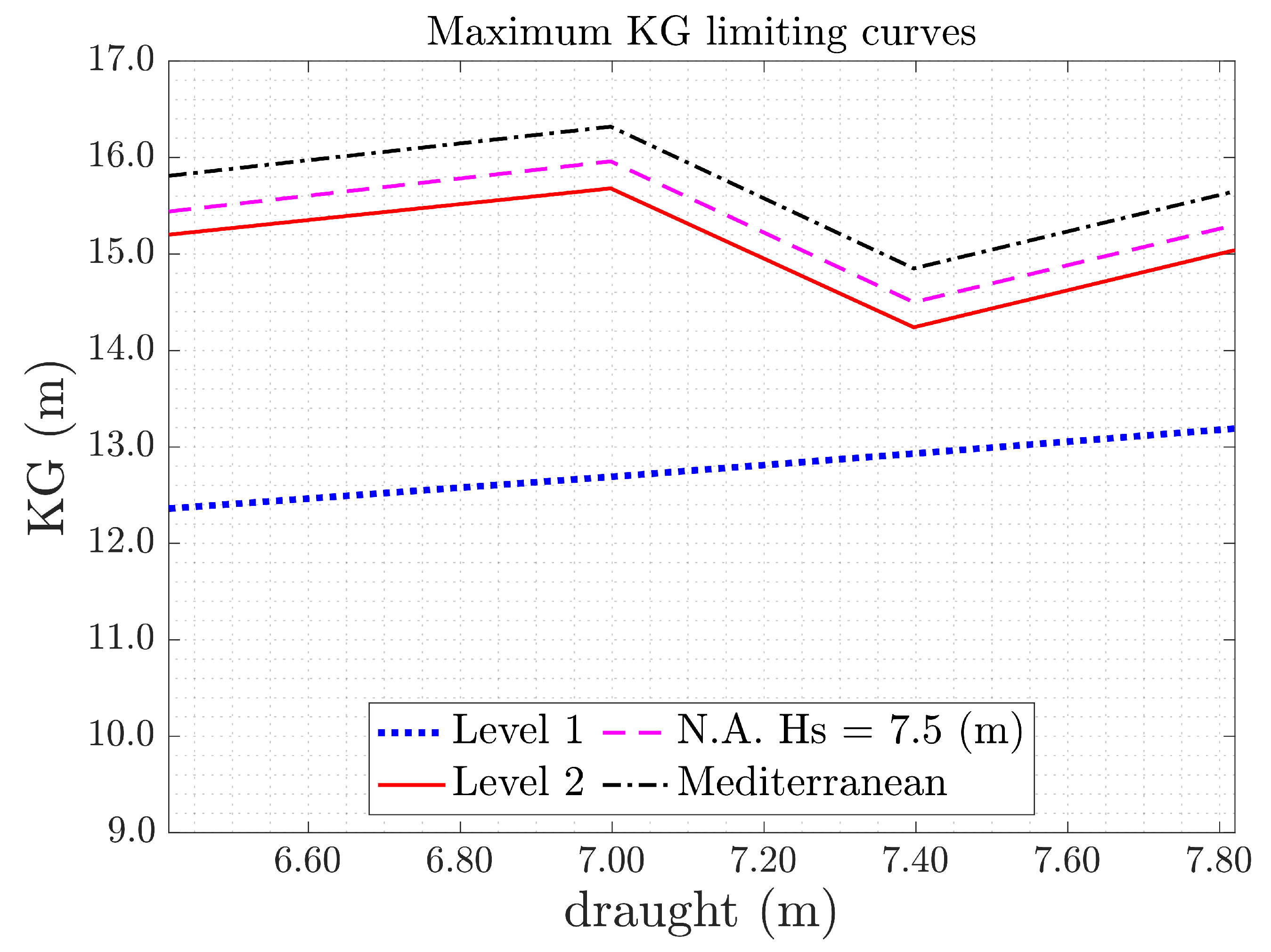
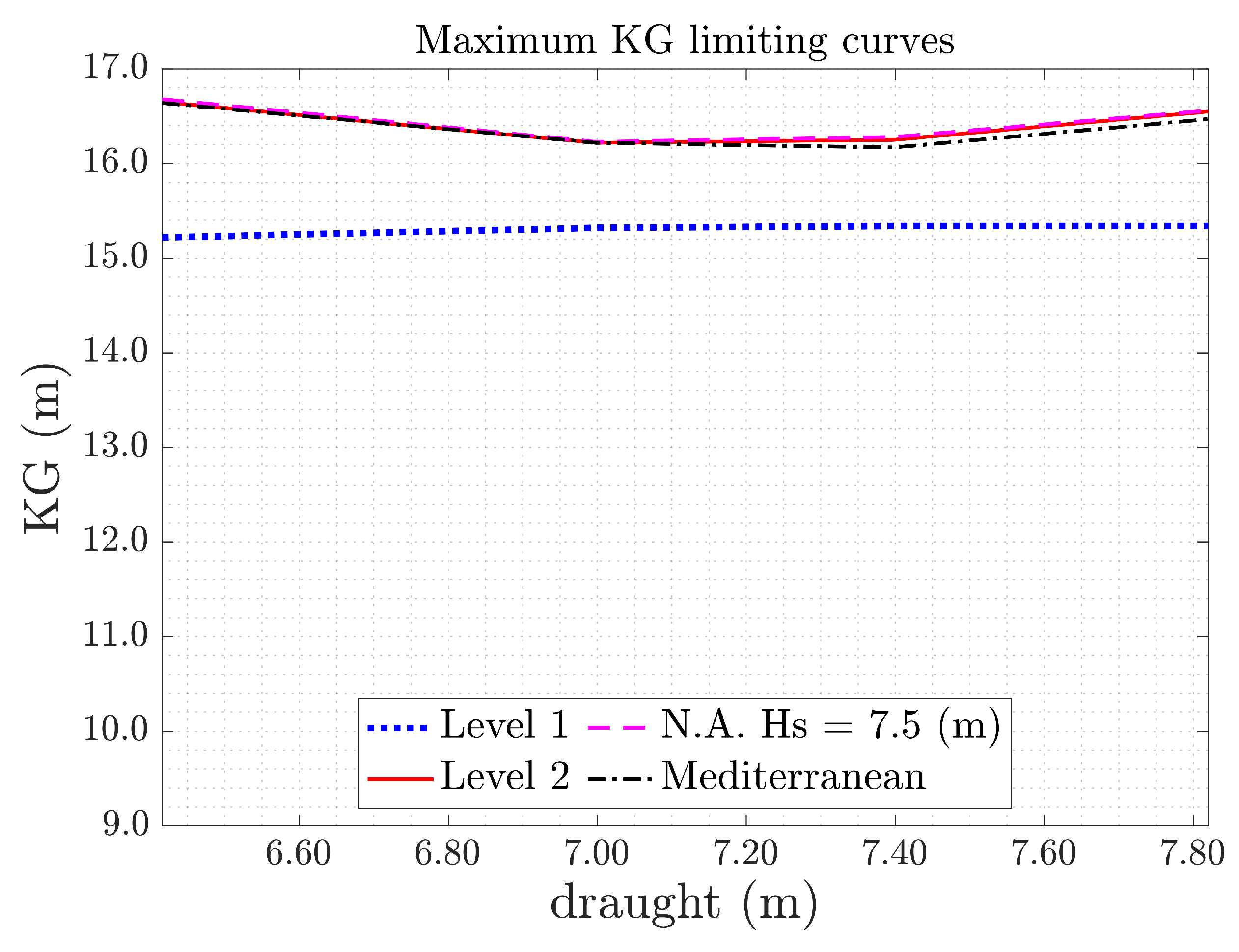
Results are presented in terms of vertical position of center of gravity (KG) limiting curves, as shown in Figure 6, Figure 7 and Figure 8. It is worth to note that results for EA are given by minimum KG curves. Drafts are presented on the horizontal axis, while the limiting KG are on the vertical axis. In each graph, the limiting curves obtained by the application of Lv1, Lv2, Lv2 with a limitation on the significant wave height and Lv2 with a limitation on the geographical area are shown. The first OL set an admissible significant wave height of ${\mathrm{H}}_{\mathrm{S}}=7.5\left(\mathrm{m}\right)$, while in the second limitation the unrestricted navigation has been replaced by a navigation confined in the Mediterranean sea.

The design domain is defined as the area below the maximum KG limiting curve (vice-versa for the minimum KG limiting curve due to EA), where the design centre of gravity of the ship may be placed safely. Outcomes point out that there is a significant difference in terms of design domain between first and second vulnerability levels. As expected, this is due to the caution factor inherent with the structure of first levels. Looking at the application of OL, it seems that no noticeable effect of these restrictions are evident on the second vulnerability level of DS. OL increases the design domain for PLS and EA; in particular for this vessel, the restriction on the geographical area gives the greatest improvement in term of KG domain range.

6. Conclusions

An overview of the SGISc has been outlined, comprehensive of the first and second vulnerability level criteria (Lv1 and Lv2), the so called direct stability assessment and the Operational Measures that in turn are inclusive of Operational Limitations and Operational Guidance. Graphical representations to better describe the mutual relation among the whole set of different rules have been provided, able to deliver the complex SGISc framework at a glance. The set of rules is the results of a very innovative trade off on different domains:

• Physically based modelling and formulation;
• Computational approach and relevant computational power needed;
• Design assessment complemented with operational support and vice-versa.

The point of strength of SGISc is the ability to introduce into the stability assessment the dynamic interactions of the ship with the environment. Nevertheless, it is to be demonstrated now that such set of rules is really and effective asset to design and operate safer ships. The calculation burden and procedure complexity in some cases are really demanding and the sensitivity of results to significant design and operational parameters is to be investigated. Therefore an intensive application campaign of this innovative set of rules is encouraged by IMO in order to possibly improve the SGISc in terms of formulations, procedures and standards.

As an example, the vulnerability assessments for pure loss of stability, dead ship condition and excessive acceleration modes have been presented; operational limitations in terms of maximum significant wave height and geographical area have been further investigated as well. Outcomes show how in this case, the consistency of the multilayered philosophy has been respected between levels of the same stability failure mode. Nevertheless, the application of OL for the dead ship failure mode shows how the influence of this option is very limited compared to other stability failure modes.

For this case study, SGISc do not imply any severe constrains to the design of the vessel. The application of OL was actually not needed for the analysed vessel, although it shows that introducing restrictions—with a relatively low-impact on the operative life of a ship (i.e., maximum admissible wave height equal to 7.5 (m))—may further enlarge the design domain available to the designer. Furthermore, a proper integration of design modifications with operational measures may lead to an improvement of ship safety without any significant issue on the project. In any case, the study and definition of OG as a support to the master represents a significant aid to the navigation. It becomes an important tool to be complemented with the master experience at sea, with the aim to further improve the ship safety performance.