Numerical Study on Regular Wave Shoaling, De-Shoaling and Decomposition of Free/Bound Waves on Gentle and Steep Foreshores

Abstract

Numerical tests are performed to investigate wave transformations of nonlinear nonbreaking regular waves with normal incidence to the shore in decreasing and increasing water depth. The wave height transformation (shoaling) of nonlinear waves can, just as for linear waves, be described by conservation of the mechanical energy flux. The numerical tests show that the mechanical energy flux for nonlinear waves on sloping foreshores is well described by stream function wave theory for horizontal foreshore. Thus, this theory can be used to estimate the shoaled wave height. Furthermore, the amplitude and the celerity of the wave components of nonlinear waves on mildly sloping foreshores can also be predicted with the stream function wave theory. The tests also show that waves propagating to deeper water (de-shoaling) on a very gentle foreshore with a slope of cot(β) = 1200 can be described in the same way as shoaling waves. For de-shoaling on steeper foreshores, free waves are released leading to waves that are not of constant form and thus cannot be modelled by the proposed approach.

1. Introduction

When waves generated offshore propagate into shallow water, wave transformation processes occur. These processes include shoaling, refraction, diffraction, wave breaking, dissipation due to bottom friction, wave reflection and wave–wave interaction. These transformation processes are key parameters to quantify for coastal engineers when designing new coastal structures. The wave height at the toe of the structure is a typical design parameter and is highly influenced by these transformation processes. The designs by the coastal engineers are often tested in small-scale tests before they are constructed in full scale. In many cases, these tests are carried out in short wave flumes and thus only shoaling, breaking, wave reflection and wave–wave interaction are relevant. As the response of most structures is related to the incident waves, it is very important to be able to estimate the incident wave train accurately. Usually, the incident wave train is obtained by separating the total waves measured at multiple locations into incident and reflected wave trains (Goda and Suzuki [1], Mansard and Funke [2], Zelt and Skjelbreia [3], Frigaard and Brorsen [4], Medina [5], Lykke Andersen et al. [6,7] and Eldrup and Lykke Andersen [8]). Reliable estimates for tests with large water depth variations within the measurement array require that shoaling is included in the mathematical model used in the wave separation method. That was done by Baldock and Simmonds [9] for linear waves only.

The present paper deals with shoaling of nonlinear regular waves with normal incidence to foreshores with parallel depth contours by numerical modelling. Existing nonlinear shoaling theories only give the shoaling of the wave height, while the application in wave separation method requires shoaling of the individual components including the bound harmonics. The shoaling theories have mainly been applied to incident waves. The shoaling process of the reflected waves is different when waves are nonlinear. When reflected waves are de-shoaling into deeper water, free waves might be released from the primary wave (see Beji and Battjes [10]). Therefore, de-shoaling processes of the reflected waves are also investigated and compared to existing shoaling theories.

2. Literature Study on Foreshore Processes for Regular Waves

The wave shoaling process is a well-known transformation process and was described by Green [11] and Burnside [12]. Green [11] described the shoaling for linear shallow water conditions while Burnside [12] extended it by using conservation of the mechanical energy flux of linear waves. Close to the coast nonlinear effects become important, but the above references provide the fundamental background for shoaling. The time-averaged energy contained in the control volume (Figure 1) should be conserved. In the absence of dissipative processes, this gives that the time-averaged mechanical energy flux trough section A should equal the time averaged mechanical energy flux trough section B.

In many cases, it is assumed that section A is on deep water, but in the present paper, the wave height ratio between any two sections A and B is referred to as the shoaling coefficient (K_s = H^B/H^A). As stated above, this can be calculated from the conservation of the mechanical energy flux:

$$E^A{c}_{\mathrm{g}}^A=E^B{c}_{\mathrm{g}}^B$$

(1)

where c_g is the energy propagation velocity, and E is the time-averaged mechanical energy per unit area in the horizontal plane. For linear waves, E is proportional to the wave height squared, and the energy propagation velocity is equal to the group velocity. Based on Equation (1), the linear shoaling coefficient K_sl can be calculated with Equations (2) and (3) (see Burnside [12]).

$$K_{\mathrm{sl}}=\frac{H^B}{H^A}=\sqrt{\frac{c_{\mathrm{g}}^A}{c_{\mathrm{g}}^B}}$$

(2)

$$c_{\mathrm{g}}=\frac{g}{2\mathsf{\omega }}\left(\tanh \left(kh\right)+\frac{kh}{{\cosh }^2\left(kh\right)}\right)$$

(3)

Here, g is the gravity acceleration, ω = 2π/T is the angular frequency. k = 2π/L is the wavenumber based on linear dispersion, h is the water depth. Above is based on linear potential wave theory on horizontal bottom and thus its validity is limited to linear waves on mild slopes and no energy dissipation.

In shallow water conditions, shoaling makes the waves higher and steeper and thus more nonlinear as h/L decreases and H/L increases. For this reason, the linear shoaling is in many cases underestimating the actual shoaling. As pointed out by Le Méhauté and Webb [13], the energy flux conservation might also for nonlinear waves be based on wave theories for horizontal seabed as long as the bottom slope is mild. This is because the terms in the bottom slope are small compared to the other nonlinear terms under mild slope conditions. Le Méhauté and Webb [13] used Stokes third-order theory to develop a formula for the nonlinear shoaling coefficient. Koh and Le Méhauté [14] extended that work to fifth-order. However, as both methods are based on Stokes theories, they are only valid for small nonlinearities with Ursell numbers, Ur = HL²/h³ < 10. Methods based on cnoidal wave theory were developed by Svendsen and Brink-Kjær [15] and Svendsen and Buhr Hansen [16], where the energy flux is calculated by linear Stokes waves in deep water followed by cnoidal waves with a transition point at h/L = 0.1. In both studies, they included only the leading terms in the energy flux for the cnoidal waves. Based also on cnoidal wave theory, Shuto [17] developed three simple equations to describe the nonlinear shoaling coefficient. The transitions between the three formulae are at Ur = 30 and Ur = 50. Shuto [17] found that, for linear waves (Ur < 30), the cnoidal wave theory was unreliable and instead the shoaling is based on linear wave theory. Kweon and Goda [18] developed a simple formula to approximate the three equations developed by Shuto [17] in one equation. Rienecker and Fenton [19], developed a shoaling method which is based on the stream function wave theory and conservation of mechanical energy flux. Rienecker and Fenton [19] used the closed-form expression for the mechanical energy flux derived by Longuet-Higgins [20] and Cokelet [21], see Equation (4).

$$F=\left(3T-2V\right)c+0.5\overline{u_{\mathrm{b}}^2}\left(I+ch\right)+c{c}_{\mathrm{E}}Q$$

(4)

Here, T and V is the kinetic and potential energy per unit horizontal area, respectively. c is the phase celerity, $c_{\mathrm{E}}$ is the time mean Eulerian velocity, $u_{\mathrm{b}}$ is the bed velocity, h is the water depth and Q is the time averaged rate of flow underneath the wave. These variables are calculated with the stream function wave theory and the details are given in Rienecker and Fenton [19].

The stream function theory is valid in all depths and thus the combination of Stokes and shallow water wave theories as used in most previous studies is not needed. Their method is based on regular wave theory of permanent form (symmetrical about the wave crest) for the horizontal seabed. Thus, it is assumed that the seabed slope is so small that there is no reflection from the seabed and that the seabed does not influence the velocity, surface elevation and pressure profiles. The same shoaling method was used by Franco and Farina [22] who additionally also studied the wave breaking angle.

Swart and Crowley [23] developed a covocoidal wave theory for regular waves on a gently sloping bottom based on an assumed covocoidal mathematical expression for the surface elevation. However, the theory has not provided very reliable estimates of the measured wave parameters (see Swart and Crowley [23]). Chen et al. [24] derived a wave theory based on a Lagrangian description of waves on sloping bottoms by using a third-order asymptotic solution. Thus, the assumption of horizontal floor is avoided, but their method is valid for linear and mildly nonlinear waves only and is therefore not suitable to study the shoaling processes of highly nonlinear waves.

Using the method by Kweon and Goda [18] or Rienecker and Fenton [19], the nonlinear shoaling coefficient K_sn in Figure 2 has been obtained. The predicted shoaling coefficient is shown as function of k₀h and H₀/L₀ where the wavenumber k₀ = 2π/L₀ is based on the deep-water wavelength L₀ = gT²/(2π). The shoaling coefficients are only shown for waves that are not breaking due to depth-induced wave breaking, which is assumed to occur at H/h ≈ 0.8 for shallow water waves on horizontal seabed (see McCowan [25] and Goda [26]). The figure shows that deviations are observed between the nonlinear shoaling coefficient by Kweon and Goda [18] and Rienecker and Fenton [19] close to the wave breaking point, but otherwise the agreement is good. It is also observed that the linear and nonlinear shoaling coefficients are almost identical for k₀h > 0.25, while for k₀h < 0.25, the nonlinear shoaling coefficient becomes significantly larger than the linear shoaling coefficient. Based on the nonlinear shoaling coefficient, it can also be observed that the shoaling coefficient is increasing with increasing offshore wave height (corresponding to higher H₀/L₀ for identical k₀h in the diagram).

When waves shoal into shallow water, their nonlinearity increases which generates higher order bound harmonics that propagate with the celerity of the primary wave component. Linear shoaling theory assumes waves remain monochromatic and can thus not predict the amplitudes of the bound higher order components. The analysis of accuracy and the validation of the shoaling coefficient estimation methods presented above have been based on the examination of the evolution of the wave height only. The stream function theory seems not to have been used to investigate the shoaling of the primary component and the bound harmonics. However, the amplitudes of the primary and the bound wave components might be calculated with stream function theory by Fenton and Rienecker [27] based on the shoaled wave height. As the Fenton and Rienecker [27] theory is valid for horizontal foreshores only, this methodology needs first to be validated for various foreshore slopes.

In order to apply a shoaling theory in a reflection separation algorithm it is also necessary to study the de-shoaling process for the reflected waves as they are propagating into deeper water. Some of the de-shoaling processes can be described from the well-known tests by Beji and Battjes [10] and Luth et al. [28]. They tested the wave transformation of regular waves propagating over a submerged bar for breaking and non-breaking wave conditions. The tests with non-breaking waves by Beji and Battjes [10] showed that incident waves passing a submerged bar would generate a complicated wave pattern behind the bar that looks like irregular waves. This pattern is caused by the incident wave decomposing into free and bound waves with different celerities and thus waves with non-constant form are generated. These wave processes have in the past been difficult to model accurately with partially nonlinear and dispersive numerical models, e.g., of Boussinesq type (see Dingemans [29]). However, these processes can be solved with fully nonlinear and dispersive models (see Raoult et al. [30]). The decomposition process has been attributed to the de-shoaling process on the leeward slope of the submerged bar. However, it was not mentioned if the horizontal part on the submerged bar releases free waves as well. Therefore, numerical tests are performed in the present study to quantify the processes that can influence the waves propagating to deeper water.

3. Numerical Study of Nonlinear Wave Shoaling

The MIKE 3 Wave Model FM by DHI has been used to propagate waves from deep water to shallow water. The model is a phase-resolving, fully nonlinear wave model that is based on the 3D Reynolds Averaged Navier-Stokes equations (RANS) with k-ε turbulence model. The free surface is described by a height function (see DHI [31]). The model has been validated against a set of typical benchmark tests which, for example, includes validation of regular wave shoaling over a submerged bar with physical tests from Luth et al. [28] (see DHI [32]).

Table 1. Test conditions at the wave generation zone.

Case	H (m)	T (s)	k0h	H/L (%)	h/L	Ur
I	0.10	2.4	2.15	1.14	0.343	0.3
II	0.10	3.7	1.10	0.58	0.175	1.1
III	0.10	5.0	0.76	0.40	0.120	2.3

shows the three sea states (cases) that have been generated at 3 m water depth. The sea states have periods of 2.4 s, 3.7 s and 5.0 s. The wave height is 0.1 m at the wave generation line for the wave periods corresponding to deep water wave steepnesses H/L of 1.1%, 0.6% and 0.4%. The numerical tests can be considered to be scale 1:20 of prototype swell conditions. The table shows for the generation zone the relative water depth k₀h, the wave steepness H/L and the relative water depth h/L, where the wavelength is calculated with linear dispersion.

The waves are then propagating on a simple straight foreshore with slopes of cot(β) = 100, 50 and 30 (see Figure 3). To avoid any wave breaking in the numerical model, the water depth at the end of the foreshore slope is set to 115% of the depth where the shoaled wave is expected to break according to the method by Goda [26]. The water depth at breaking (h_b) is dependent on the deep water wavelength and the foreshore slope. The obtained value of H/h is 0.76–0.87 at the end of the foreshore slope. According to Goda [26], the waves are in the tested conditions breaking at 0.77 < H/h < 0.88 depending on the wave steepness and foreshore slope. The waves are always normal to the shore, i.e., no refraction occurs.

The model is discretized into ten equidistant vertical layers, and the horizontal cell size is Δx = L_end/200, where L_end is the wavelength based on linear wave theory of the primary component with the water depth at the end of the foreshore slope. The critical CFL number is set to 0.4. The data is sampled at 50 Hz. A relaxation zone behind the generation line is used to generate and absorb any reflected waves, and at the end of the flume, an effective sponge layer is used to absorb the incident waves. The generated regular waves are based on stream function wave theory.

Figure 4 shows the shoaling of the wave height from a water depth of 3 m to the water depth at the end of the foreshore slope on the three different foreshore slopes. The results are compared to the predicted wave height shoaling with linear (Equation (2)) and the nonlinear shoaling theories by Kweon and Goda [18] and Rienecker and Fenton [19]. The figure shows that for Case II and Case III the wave height is increasing throughout the entire slope, while for Case I the wave height is decreasing before it starts to increase. The overall pattern is as presented in Figure 1, as the observed difference is due to the different k₀h values at the generation point. Case II and Case III are in the numerical model not generated in deep water, but instead, in intermediate water and for this reason, the drop in wave height is not observed.

Furthermore, the numerical results show that the shoaling of the wave height is only slightly dependent on the foreshore slope as also predicted by the shoaling theories. For Case I, the linear theory significantly underestimates the shoaling for k₀h < 0.35, and the nonlinear method by Kweon and Goda [18] slightly underestimates for k₀h < 0.21. The nonlinear method by Rienecker and Fenton [19] fits well to the numerical results, but for H/h ≈ 0.69 the stream function wave theory breaks down due to the assumption of horizontal seabed. For Case II and Case III, there is a significant underestimation with the linear theory for k₀h < 0.20 and k₀h < 0.17, respectively. The nonlinear shoaling theory by Kweon and Goda [18] slightly underestimates the wave height for k₀h < 0.15, while the method by Rienecker and Fenton [19] fits better to the numerical results where deviations are to be explained by the fact that vertical asymmetric waves have less energy than symmetrical waves with the same height. It is though not consistent in the sense that the steepest foreshore (cot(β) = 30) causes the most asymmetric waves, but not always the highest shoaling. Thus, also reflections from the seabed for the steeper slopes are probably affecting the results.

The wave parameters at the water depth at the end of the foreshore slope in Figure 4 can be seen in

Table 2. Test conditions at the end of the foreshore slope.

Case	T (s)	Foreshore Slope, cot(β)	h (m)	H (m)	k0h	H/L (%)	h/L	Ur
I	2.4	100	0.215	0.167	0.40	4.91	0.063	194.1
		50	0.211	0.169	0.39	5.02	0.063	204.2
		30	0.204	0171	0.39	5.16	0.062	221.3
II	3.7	100	0.276	0.220	0.29	3.66	0.046	377.7
		50	0.271	0.229	0.29	3.85	0.046	407.9
		30	0.264	0.229	0.28	3.90	0.045	430.2
III	5.0	100	0.325	0.248	0.23	2.80	0.037	566.2
		50	0.320	0.263	0.23	2.99	0.036	619.6
		30	0.312	0.253	0.23	2.92	0.036	627.2

. The table shows that the relative water depth number k₀h has decreased significantly compared to the generation point at h = 3 m (Table 1), indicating that the nonlinearity has increased as well.

Figure 5 shows the surface elevation, the wave amplitudes and the phase difference between the primary component and the bound higher order harmonics for Case III. The phase is not shown for amplitudes less than 5 mm as the uncertainty on the phase is too large. Results are shown for the three different foreshore slopes and at three different water depths. The surface elevation clearly shows that the vertical asymmetry of the waves increases as the foreshore slope increases. The vertical asymmetry is typically described by the atiltness factor (see Goda [33]) (Eq. 10.138). Adeyemo [34] also found that the vertical asymmetry is increasing for increasing foreshore slope and also when the relative water depth h/L decreased (i.e., increasing nonlinearity). In the bottom of Figure 5, the phase difference of the bound higher order components and the primary component is given. For a nonlinear regular wave with no vertical asymmetry, the phase difference is zero according to the stream function wave theory. The present results show that the phase difference is largest for the steepest foreshore slope which increases the vertical asymmetry and thus the results are in line with the study by Adeyemo [34]. However, it is observed that the wave at h = 0.36 m and foreshore slope cot(β) = 100 has smaller phase difference compared to the results at h = 0.60 m. The smaller phase difference is not seen for the steeper foreshore slopes. Figure 5 also shows that the amplitude of the primary component increases with increasing foreshore slope and that the higher order components decrease, thus non-breaking waves on gentle slopes are more nonlinear than on steep foreshores.

Figure 6 shows the same parameters as Figure 5, but for Case I. The results are similar to Figure 5, but the conclusions are not as clear since the nonlinearity of the wave is much smaller.

It has been shown that the shoaling of the wave height is mostly independent on the foreshore slope, but the foreshore slope and wave nonlinearity influence the wave amplitudes and phases. Therefore, it is not expected that the amplitudes can be very accurately estimated if the foreshore slope and nonlinearity are disregarded, but as a starting point for including shoaling in a reflection analysis on sloping foreshores, it might be reasonable as the shoaling distance (the length of the wave gauge array) is limited.

3.1. Procedure for Shoaling of Wave Components

The calculated shoaling coefficient gives the shoaling of the wave height, but the shoaling of the individual components (primary and bound superharmonics) is also studied. Using linear theory, only a primary component exists, and thus the shoaling coefficient for the primary component is identical to the shoaling of the wave height. This is not the case for nonlinear waves where the shoaling of the primary and higher order components instead is estimated with the stream function wave theory by Fenton and Rienecker [27]. For a given wave height the stream function, wave theory predicts the amplitudes of each wave component and thus the shoaling of the individual components may be estimated under the assumption that the bottom slope is small and that the nonlinear shoaling method by Rienecker and Fenton [19] is reliable.

Figure 7 shows the numerical modelled and predicted amplitudes for the three different foreshore slopes. The numerical amplitudes are oscillating, and this is especially seen on a₁ for Case III on the steep slope. Closer examination reveals that the wavelength of the oscillations equals half the length of the incident waves. Thus, the oscillations are very likely caused by partial nodes and antinodes due to the reflection from the seabed. An additional argument for this explanation is that the amplitude of the oscillations is highest for low steepness waves on steep foreshores. The oscillations are also much smaller for the higher order components as the reflected waves are almost linear.

For a₁ the nonlinear method is a closer match to the numerical modelled amplitude for all foreshore slopes compared to the linear method. The nonlinear method is very accurate both for the primary component as well as for the bound harmonics for the foreshore slope cot(β) = 100. The agreement even seems better for the individual components than for the wave height given in Figure 4. However, a closer examination reveals that all the higher order harmonics amplitudes are slightly higher in the numerical model than predicted by the shoaling theory. For the steeper foreshore slopes, the deviations on the individual components are higher as the shoaling theories use the kinematics of waves on horizontal foreshore to calculate the mechanical energy flux. Thus, for slopes of cot(β) ≤ 50, the vertical asymmetry is very important when the wave nonlinearity becomes high. In Figure 5 and Figure 6 this was also demonstrated as increasing foreshore slopes cause less high harmonic energy and more primary energy. The deviations between the numerical modelled and predicted amplitudes by the nonlinear shoaling method are mainly due to accumulation of small errors over large distance. If the present results are used in a wave separation method the errors are less relevant as they accumulate only over a small distance (the length of the wave gauge array is typical 45% of the dominant wavelength, see Eldrup and Lykke Andersen [8]).

3.2. Procedure for Wave Component Celerity

As long as no free incident waves and reflected waves exist, all the components in a regular wave have a constant celerity on a given depth. This constant celerity is decreasing with depth and is increasing with the wave nonlinearity. The latter is known as the amplitude dispersion and Lykke Andersen et al. [6] concluded that this is important for wave separation of highly nonlinear waves. They used the predicted celerity from the stream function theory by Fenton and Rienecker [27]. The Fenton and Rienecker [27] method is valid for horizontal foreshore, but in the present work, it is investigated if the method can be used to estimate the celerity for waves on a sloping foreshore when the local depth is used. The celerity in the numerical model data is found by Equation (4).

$$c\left(x_i\right)=\frac{(x_{i+\alpha }-x_{i-\alpha })}{\Delta t}$$

(5)

here, c(x_i) is the celerity at grid cell number i with coordinate x_i, Δt is the time difference of the numerically modelled surface elevation between grid cells number i + α and i − α with coordinates x_i+α and x_i−α. Δt is obtained by using a cross-correlation analysis between the signals at x_i+α and x_i−α. α = 3 is used to calculate average values over several grid cells. The signal has been resampled to 5000 Hz to reduce the uncertainty of the calculated Δt from the cross-correlation analysis.

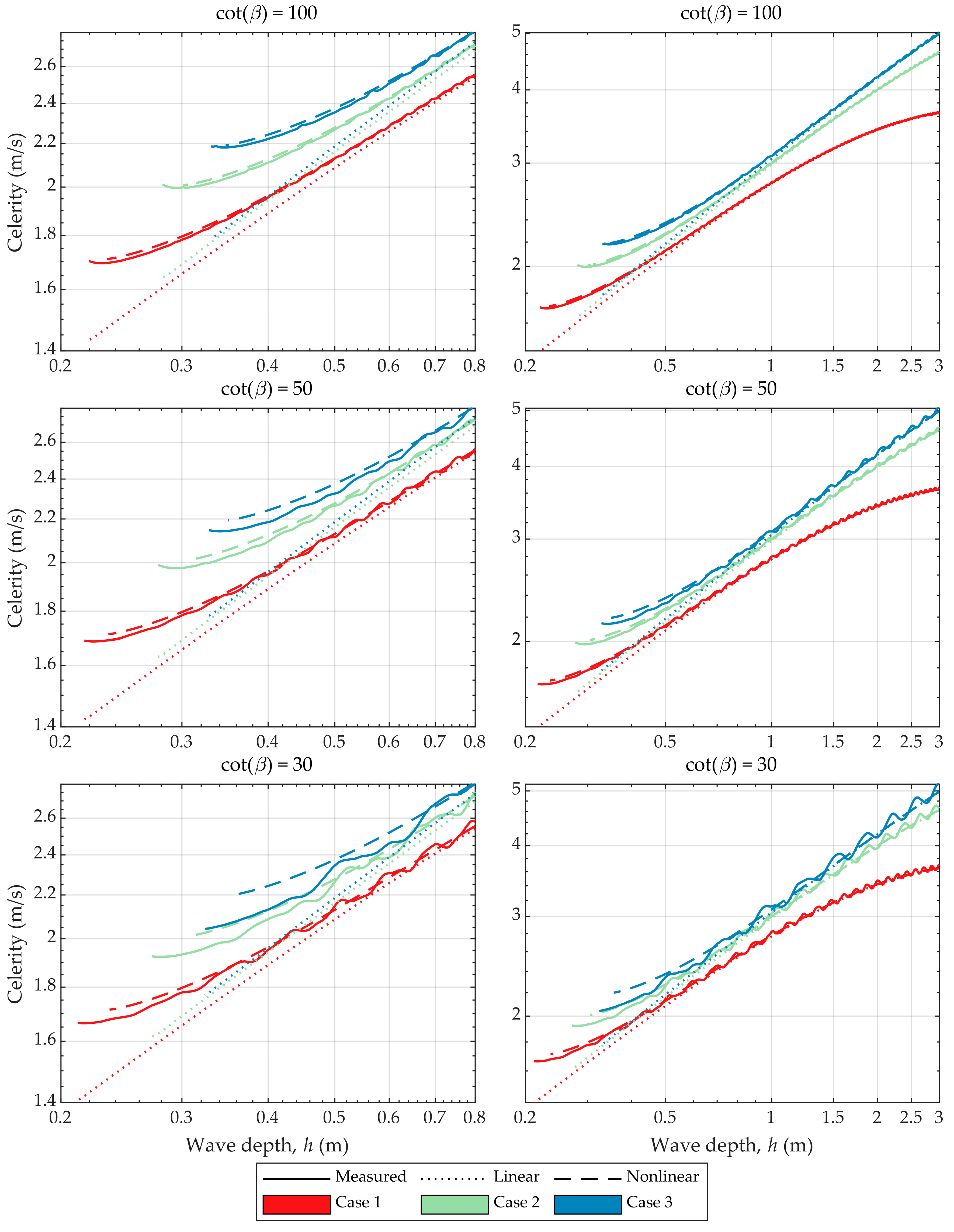
Figure 8 shows the numerical modelled and predicted celerity of the wave on the three foreshore slopes. Predictions by linear wave theory and stream function theory for nonlinear waves by Fenton and Rienecker [27] are also shown. The predicted celerity by both methods is almost identical until a water depth of h ≈ 1 m. For water depths smaller than h ≈ 1 m, the predicted celerity with linear theory is smaller than the one with nonlinear theory. As for the amplitudes, the numerical modelled celerity shows oscillations for the steep slopes, which is most likely due to reflection from the seabed. Disregarding the oscillations of the numerical modelled celerity, then, it is clear that foreshore slopes do have a very minor influence on the celerity in the numerical model results. In shallow water, the celerity in the numerical model is slightly smaller than the stream function theory predictions. These deviations are highest for the steepest foreshore slope and might thus be an influence of the slope on the celerity. Similar observations were found by Li et al. [35], which showed that the phase celerity decreases with increasing foreshore slope. Lower celerity must result in higher wave height in order to have the same mechanical energy flux. Thus, part of the observed deviations on the wave height shoaling might be caused by the lower celerity. The results show that the celerity based on Fenton and Rienecker [27] is a reasonable estimate of the wave celerity for sloping foreshores.

3.3. Shoaling Process Conclusion

A methodology has been found to describe shoaling of the components of nonlinear incident regular waves on a constant foreshore slope. The methodology is based on stream function wave theory for horizontal foreshore. For a foreshore slope of cot(β) = 100 the methodology was found very accurate, while inaccuracies increase with increasing foreshore slope. This is expected to be caused by the fact that the stream function wave theory assumes horizontal seabed leading to vertical symmetric waves and no reflection. On sloping foreshores, waves are vertical asymmetric and reflection from the seabed occurs. The overall conclusion is that the shoaling of the incident waves on a constant slope is well described with above methodology when the relative water depth h/L is larger than the value given in

Table 3. The lower limit for the relative water depth to which the present shoaling methodology is valid.

Foreshore Slope, cot(β)	h/L
100	0.036
50	0.073
30	0.085

for a given foreshore slope. For the mildest slope, the methodology is valid up to the lowest studied relative water depth in the numerical tests. Thus, the lower limit of h/L given in Table 3 for the mildest foreshore slope is conservative and a lower limit might be found if waves of higher nonlinearity are studied.

4. Numerical Study of Nonlinear Wave De-Shoaling

Before the de-shoaling of reflected waves can be included in a wave separation method, deeper insight of the de-shoaling process of the reflected waves is needed. The de-shoaling process can consist of additional processes, for example, release of free waves as demonstrated by Beji and Battjes [10]. Therefore, new numerical tests are performed to investigate the wave transformation of the de-shoaling waves.

4.1. Wave De-Shoaling

Figure 9 shows a setup with a simple straight slope where the generated waves are highly nonlinear and are propagating to deeper water. The waves are generated with stream function wave theory with a wave height of H = 0.168 m and T = 5 s corresponding to the wave at h = 0.5 m in the previous setup for foreshore slope cot(β) = 30. If the wave de-shoaling is identical to the shoaling, then the results at h = 3 m should be a close match to the generated waves at h = 3 m in the previous section. The generated waves at the boundary are in the present case assumed vertical symmetric and not vertical asymmetric as found in Section 3.

Free waves with smaller wave periods than the generated wave might exist in the deep part of the model if the de-shoaling is not identical to the shoaling. This is accounted for in the discretization of the model and thus 20 equidistant vertical layers are used. The horizontal cell size is Δx = L_0.5m/200, where L_0.5m is the linear wavelength in 0.5 m water depth of the primary component. The critical CFL number is set to 0.4. The data is sampled at 50 Hz. A relaxation zone behind the generation line is used to generate and absorb any reflected waves and at the end of the flume, an effective sponge layer is used to absorb the incident waves.

Figure 10 shows the numerical modelled and the predicted amplitude by using the nonlinear shoaling coefficient by Rienecker and Fenton [19] and the predicted amplitudes with the method by Fenton and Rienecker [27]. When the waves de-shoal they become less nonlinear and thus bound energy will shift to other components. Under some circumstances, this energy is mainly shifted to the primary component, but under other circumstances it leads to large higher harmonic free waves. The results show that, for a foreshore slope of cot(β) = 1200, the numerical modelled and the predicted amplitudes are a close match and thus the de-shoaling is identical to the shoaling process and no free energy is released. Thus, all the bound higher harmonic energy is transferred to the primary component during de-shoaling. However, for the other foreshore slopes this is not the case as instead the primary amplitude is less than predicted and the amplitudes of the higher harmonics is larger than predicted. For the foreshore slope with cot(β) = 100, a₁ is only slightly smaller than predicted using the nonlinear shoaling theory and some small oscillations are observed in the numerical model results. More important is that a₂ and a₃ deviate significantly even for a mild slope of cot(β) = 100. At h = 3 m, significant energy is still present at the 2nd and 3rd harmonics indicating they have been released as free waves. For the foreshore slope with cot(β) = 30, these two effects are more visible indicating that the steeper the foreshore slope, the more energy is released into free waves and less energy is being transferred to the primary component. Thus the reason for the deviations on the steeper foreshores is release of free waves as also found by Beji and Battjes [10] for very steep slopes. The free waves also explain the strong oscillations of the amplitudes with x-coordinate as both bound and free energy exist at the same frequency. As the free and bound components have different celerities, the total amplitude at that frequency will vary depending on the phase of the two components at the specific coordinate. The release of free waves is investigated further in the present paper so that a reliable de-shoaling method can be established.

4.2. Wave Decomposition of Free/Bound Energy

A new model setup with a horizontal plateau at the crest of a submerged bar is tested (see Figure 11). The bathymetry is chosen as cot(β) = 30 for the foreshore slopes as the results in Figure 10 showed that a steep foreshore generates a significant amount of free waves. The new setup is seen in Figure 11. The discretisation of the model is the same as in Section 4.1.

The horizontal part avoids further shoaling, but the waves have to adapt to the new horizontal foreshore. This adaption process might lead to free waves being generated as the waves have shoaled into vertical asymmetric waves and should evolve toward vertical symmetric waves at the horizontal foreshore. For the following analysis, it is assumed that this adaptation has taken place after 100 m and thus the following 280 m (x = 225–505 m) is used to analyze the free and bound wave components. Assuming that several wave components exist at the horizontal crest and wavenumbers, amplitudes and frequencies are constant in time and space, it is possible to estimate these wave components by a two-dimensional Fourier transformation (2DFFT). The used FFT is based on the work by Frigo and Johnson [36]. This analysis can show if any free waves are generated when the slope of the foreshore changes. A time window of 30 periods has been selected for the analysis and thus the primary and harmonic components are all periodic in the selected time window. As both bound and free waves might exist with various wavelengths it was instead for the spectral domain decided to use a 10% Tukey (cosine) taper window in each end.

Free waves might also be released when the waves propagate from the horizontal part to the leeward side of the submerged bar due to the slope transition and de-shoaling processes. It is not expected that further free waves are released at the intersection between the leeward side of the submerged bar and the horizontal part behind the submerged bar since the nonlinearity of the waves is small and is no longer significantly influenced by the seabed. The horizontal part behind the submerged bar is used to investigate if any bound waves or free waves still exist after the de-shoaling process by applying 2DFFT also at this part.

Figure 12 shows the amplitudes with respect to the wavenumber and wave frequency for the setup in Figure 11. Figure 12a shows the results for the horizontal part on the submerged bar (x = 225–505). The red line shows components with the same celerity as the primary wave that is generated with a frequency of 0.2 Hz. On the red line, the bound higher order harmonics are thus also observed. The 2DFFT detects the high energy both at the primary component and at the 2nd and 3rd bound harmonics. The black line shows the linear dispersion relation, which means that small amplitude free waves would be located on the black line. The components placed at 0.4 and 0.6 Hz on the black line are free waves that are released on the horizontal top part of the submerged bar. If these free waves had any bound higher order harmonics, they would be located on the green and blue line. These free waves are not highly nonlinear, and therefore no significant higher order components are bound to these free waves. The free waves and the primary wave interact with each other and thereby subharmonics and superharmonics are generated according to third-order irregular wave theory. These interactions between the primary wave and the free waves are shown with red circles.

Figure 12b shows the results at the horizontal part after the submerged bar (x = 700–980). The figure shows only one component on the red line, and thus all the bound superharmonic energy has been moved to other components due to the decrease in wave nonlinearity during de-shoaling. A significant amount of free energy is found at 0.4 Hz (located at the black line) and it seems to have increased during the de-shoaling process indicating release of additional free energy on the leeward slope of the submerged bar. The amplitude of the free wave component at 0.6 Hz has also increased which indicates release of third order energy. Thus, the waves after de-shoaling include free energy at the frequencies of the primary component and the bound components. The nonlinearity has decreased so that the bound subharmonics and superharmonics have vanished. The transfer of energy from the bound components to the free components is complicated. To better understand this, further numerical and/or physical model tests should be performed with different foreshore slopes and wave nonlinearities in order to establish a better understanding with the final goal of establishing a mathematical model for the de-shoaling. Additionally, the knowledge on the interaction of the incident and reflected waves is very limited but might be needed for accurate description of the shoaling and de-shoaling under reflective conditions.

5. Conclusions

Numerical model tests have been carried out to study the shoaling and de-shoaling process of regular waves. Under the assumption of conservation of the mechanical energy flux, existing linear and nonlinear shoaling theories are evaluated. It was found that the shoaling of the wave height can be described with a nonlinear shoaling coefficient by Rienecker and Fenton [19]. The amplitudes and the celerity of the wave components can be described for shoaling waves with the stream function wave theory by Fenton and Rienecker [27], but some deviations are found for steeper foreshore slopes. Applicability ranges for the present shoaling methodology have been given as a function of the relative water depth h/L and foreshore slope. The applicability ranges might be extended to cover a larger range of relative water depths if a reliable wave theory valid for sloping seabed and highly nonlinear waves is developed, but until then, the best alternative is to use methods for highly nonlinear waves over horizontal seabed, e.g., the Rienecker and Fenton [19] method.

In order to study the release of free waves during de-shoaling, additional numerical model tests were performed with a simple straight slope from shallow to deep water, and tests with a submerged bar with a horizontal plateau. A similar setup was studied by Beji and Battjes [10] and they found that free waves are released from the primary wave when propagating to deeper water. The present tests with a simple straight slope showed that no free waves were released when the slope was very gentle (cot(β) = 1200). In that case, the de-shoaling followed the same processes as for the shoaling waves and could be described with the nonlinear methods by Rienecker and Fenton [19] and Fenton and Rienecker [27]. For the steeper slopes, cot(β) = 100 and cot(β) = 30, the shoaling predictions deviated from the numerical results due to release of free waves. Based on the numerical tests with the submerged bar, it was observed that free waves were released on the leeward slope of the submerged bar, which is in agreement with the observations by Beji and Battjes [10]. However, the present study showed that free waves were also released from the primary wave at the horizontal part of the submerged bar. The present study shows that free waves are released when nonlinear waves propagate on a bathymetry with sudden changes in slope that cause large deviation in the equilibrium surface profile (e.g., in the vertical asymmetry).

It was found that the free waves that are released interact with the primary wave and thereby subharmonics and superharmonics may be generated as it happens for an irregular sea state. The interactions observed in the present study can be described with third-order wave theory, but for more nonlinear cases higher order irregular wave theory might be needed.