Communicating Simulation Outputs of Mesoscale Coastal Evolution to Specialist and Non-Specialist Audiences

Abstract

Coastal geomorphologists and engineers worldwide are increasingly facing the non-trivial challenge of visualising and communicating mesoscale modelling assumptions, uncertainties and outcomes to both coastal specialists and decision-makers. Visualisation of simulation outcomes is a non-trivial problem because the more abstract scientific visualisation techniques favoured by specialists for data exploration and hypothesis-testing are not always as successful at engaging decision-makers and planners. In this paper, we show how the risk of simulation model outcomes becoming disconnected from more realistic visualisations of model outcomes can be minimised by using the Coastal Modelling Environment (CoastalME). CoastalME is a modelling framework for coastal mesoscale morphological modelling that can achieve close linkages between the scientific model abstractions, in the form of lines, areas and volumes, and the 3D representation of topographic and bathymetric surfaces and shallow sub-surface sediment composition. We propose and illustrate through the study case of Happisburgh (eastern England, UK), a transparent methodology to merge the required variety of data types and formats into a 3D-thickness model that is used to initialise a simulation. We conclude by highlighting some of the barriers to the adoption of the methodology proposed.

1. Introduction

One of the grand challenges facing coastal geomorphology today is to improve our ability to make quantitative predictions of morphological change at a scale that is relevant to longer-term strategic coastal management [1]. Following [2], this scale is herein referred to as the mesoscale, and is characterised by time horizons of the order 10¹ to 10² years and less rigorously imposed spatial dimensions of the order 10¹ to 10² km. Coastal engineers additionally face the challenge of achieving project approval which, amongst other activities, involves delivering such predictions of coastal change within an uncertainty framework that is robust enough to be useful to management and policy thinking [3]. Approval for coastal engineering schemes is granted only after the ‘stakeholders’—a diverse group of people that typically includes representatives of governments, owners, directly and indirectly affected individuals and groups, and other individuals or groups who believe they may be impacted—have had the opportunity to express their reactions [3]. In this context, both coastal geomorphologists and engineers (i.e., specialists) increasingly face the non-trivial challenge of visualising and communicating the mesoscale modelling assumptions, uncertainties and outcomes to generally non-specialist decision-makers. A key aspect of this challenge is the overarching requirement that the application of any environmental model to decision making should be transparent and reproducible, as well as adequately representing the real system properties and behaviours [4,5,6,7]. Fulfilling these requirements often requires iterative communication at different stages of the simulation process.

Within the wider context of a simulation study [8], Figure 1 illustrates an idealised workflow for the simulation of mesoscale coastal geomorphological change to inform strategic coastal management and facilitate project approval. This includes seven main activities, four of which are development-related and three of which are concerned with the validation of the model. The four development activities are: (D1) knowledge acquisition; (D2) quantitative modelling (which integrates conceptual modelling, prototyping and model coding); (D3) experimentation, and; (D4) implementation. The outcome of each process is, respectively, a system description (i.e., Coastal System Maps (CSM) and Causal Loop Diagrams (CLD) [9,10]), a digital model, solutions to the problem modelled and/or a better understanding of the real world and improvements of the real world. The three validation activities encompass (V1) structural, (V2) behaviour and (V3) policy validity testing [11]. The outcome of each validation activity is an increase/decrease in the confidence level regarding the model scope and level of detail, model behaviour and the implications of the modelling results for policy, respectively. The double arrows in Figure 1 reflect the iterative nature of the process and the circular flow of these four main activities illustrates the potential to repeat the process of improvement through multiple simulations. In this work, our interest is on model content, in particular ensuring that the model has a sufficient level of detail for the behaviour validity testing (V2) and the policy validity testing (V3). It is useful to distinguish between the realistic and useful detail that can be included in relation to topography and sedimentology and the quite abstract representations of the processes governing geomorphological development that often underpin such mesoscale simulations.

Visualisation of simulation outcomes is a non-trivial problem because the more abstract techniques generally favoured by technical specialists for data exploration and hypothesis-testing are not always successful at engaging decision-makers and planners [12]. A general perception amongst planners and managers appears to be that the more detail within a visualisation, the more accurate and believable it is [13]. However, the inclusion of detail in visualisations of the outputs of relatively abstract models is problematic and potentially misleading. This raises the danger that the mismatch between the ‘supply’ of credible model data and the user-driven ‘demand’ for realistic information may lead to a divergence between the processes of model-based simulation and the visualisation of the outputs. This difficulty arises because the digital visualisation needs to be both scientifically credible but also provide sufficient detailed information at a level of realism that decision-makers believe is most suitable. Thus, although visualisation has become a valuable part of the geo-information toolkit, caution and agreed visualisation standards are still needed. Specifically, how do we best combine different knowledge and data sets into the modelling, and how do we best visualise the model outcomes for both the coastal specialist and non-specialist?

While sub-surface geology has long been recognised as an important factor for mesoscale coastal evolution [14], the problem of ensuring that the model has a sufficient representation of the sub-surface has often been approached in an ad-hoc way that makes it difficult to trace-back to the original geological data. For example, the modelling tool used by [12] to simulate the evolution of the soft cliff coastline of Norfolk, eastern England (UK), was the Soft-Cliff and Platform Erosion (SCAPE) model code [15], which uses data on geological composition and strength, among other input data. The relatively complex geology of the East Anglian coastline was characterised in the SCAPE model through the optimisation of rock strength and the scaling factor of a longshore sediment transport calibration parameter [15]. Informed by the cliff sediment size composition (i.e., proportions of mud, sand and gravel) provided by [16] and digitised historic maps, the SCAPE model was calibrated to accurately represent first an 87-year hindcast of cliff toe evolution [15] and then a longer 117-year simulation [17]. This model was later used to predict cliff change over 100 years under a range of potential coastal management strategies for North Norfolk Council, as part of the 2013 Cromer to Winterton Ness Coastal Management study [18] to inform the selection of a preferred coastal management strategy. In that example, the mismatch between the abstract representation offered by the SCAPE model and the end-user desire for visualisations with plausible detail was met by superimposing the projected recession on the observed baseline cliff position, retaining some of the detail of that cliff-line. In this way, a mismatch was introduced between the model output and the basis of the visualisation.

Cliff sediment yields [16] were estimated from the lithology exposed at the cliff face in 1995 and represent the yields of a 1m recession of the cliff face. This was assumed, without detailed empirical evidence, to be a good representation of the inland geology. As shown by [19], it is now possible to more accurately estimate the sediment yields of an eroding cliff and shore platform. Reducing the uncertainty on cliff yields is key as they determine the beach volume, which is related to the rate of cliff recession (i.e., annual cliff top recession rate decreases exponentially with the beach volume) [20]. In addition, the inclusion of more complete data on known geology and its sediments provides a means of introducing realistic localised detail into model simulations and the visualisation of the resulting projections, which can help to satisfy the demands of end-users.

The aim of this paper is to illustrate how closely linking the outputs from the Coastal Modelling Environment (CoastalME) [16] and Geographical Information System (GIS) data structures and output formats minimises the mismatch between scientifically sound model results and user-demanded realism in terms of how the coast is represented. To demonstrate the communication of complex beach-shore platform-cliff interactions to both specialist and non-specialist audiences, we have used the simulation outcomes obtained by [19] for the eroding coast of Happisburgh (eastern England, UK). Happisburgh provides an excellent example of how superficial geology mediates the observed rapid acceleration in cliff retreat after the removal of coastal defences [21,22]. We then briefly present CoastalME as an appropriate framework to create realistic representations of coastal landform complexes including sub-surface and digital elevation data. In particular, we present the CoastalME data structure and the workflow for the initialisation of a coastal simulation model. Then we briefly describe the workflow and simulation outcomes followed by [19] when simulating one year of the evolution of Happisburgh. We then illustrate different ways of visualising the simulation outcomes, from traditional cliff lines and profiles to evolving DEMs. Finally, we discuss how this novel workflow and visualisation is an improvement relative to previous and current practices.

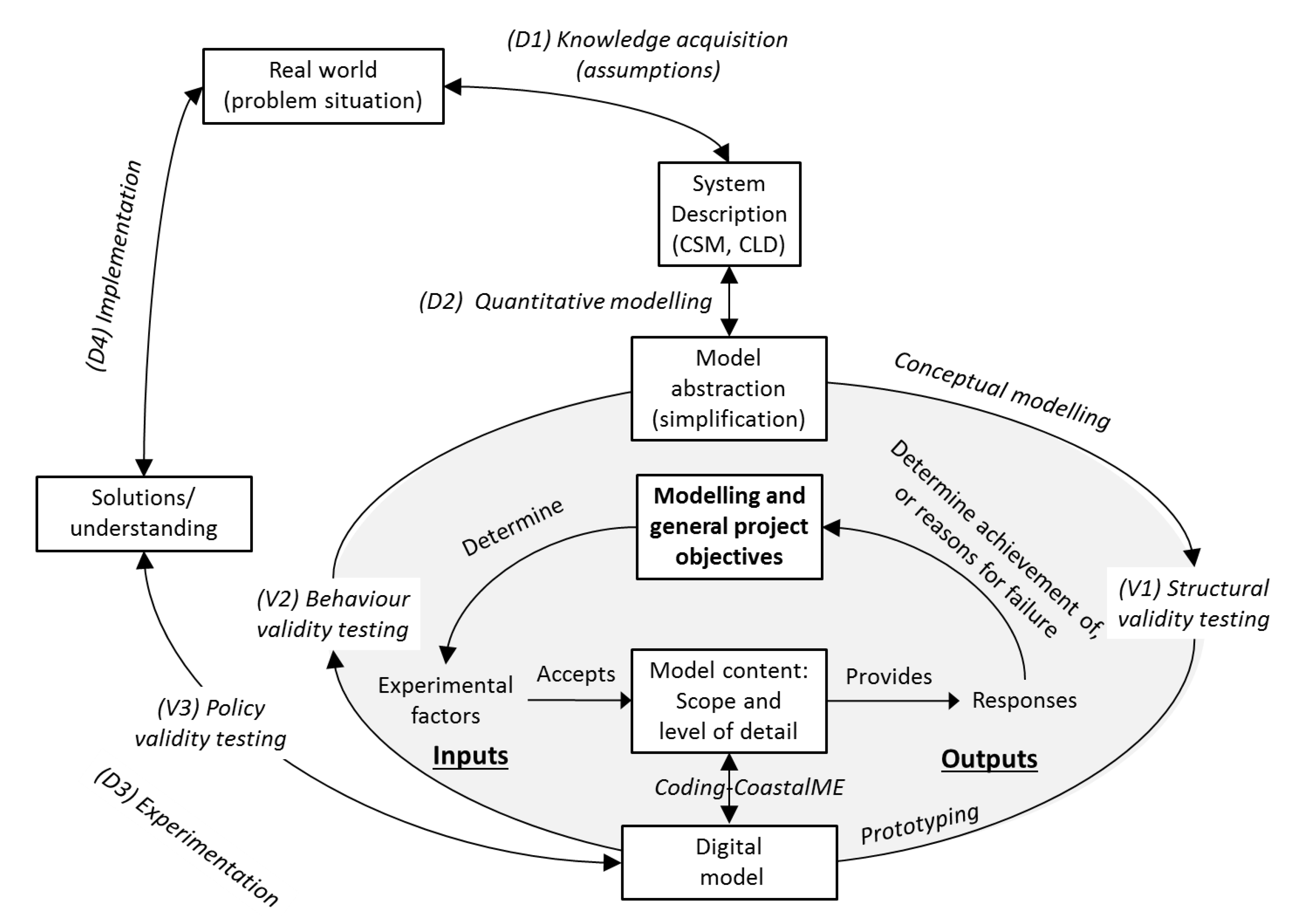
2. Materials and Methods

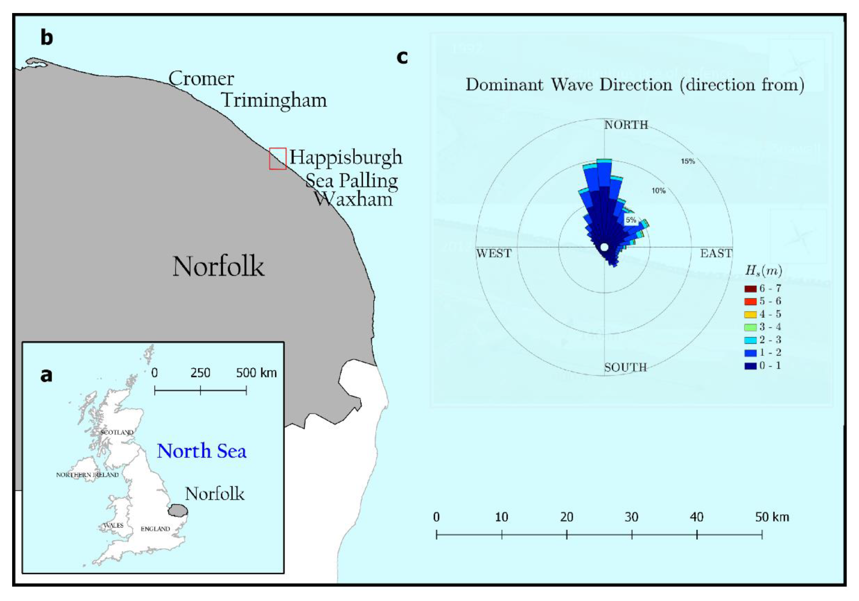
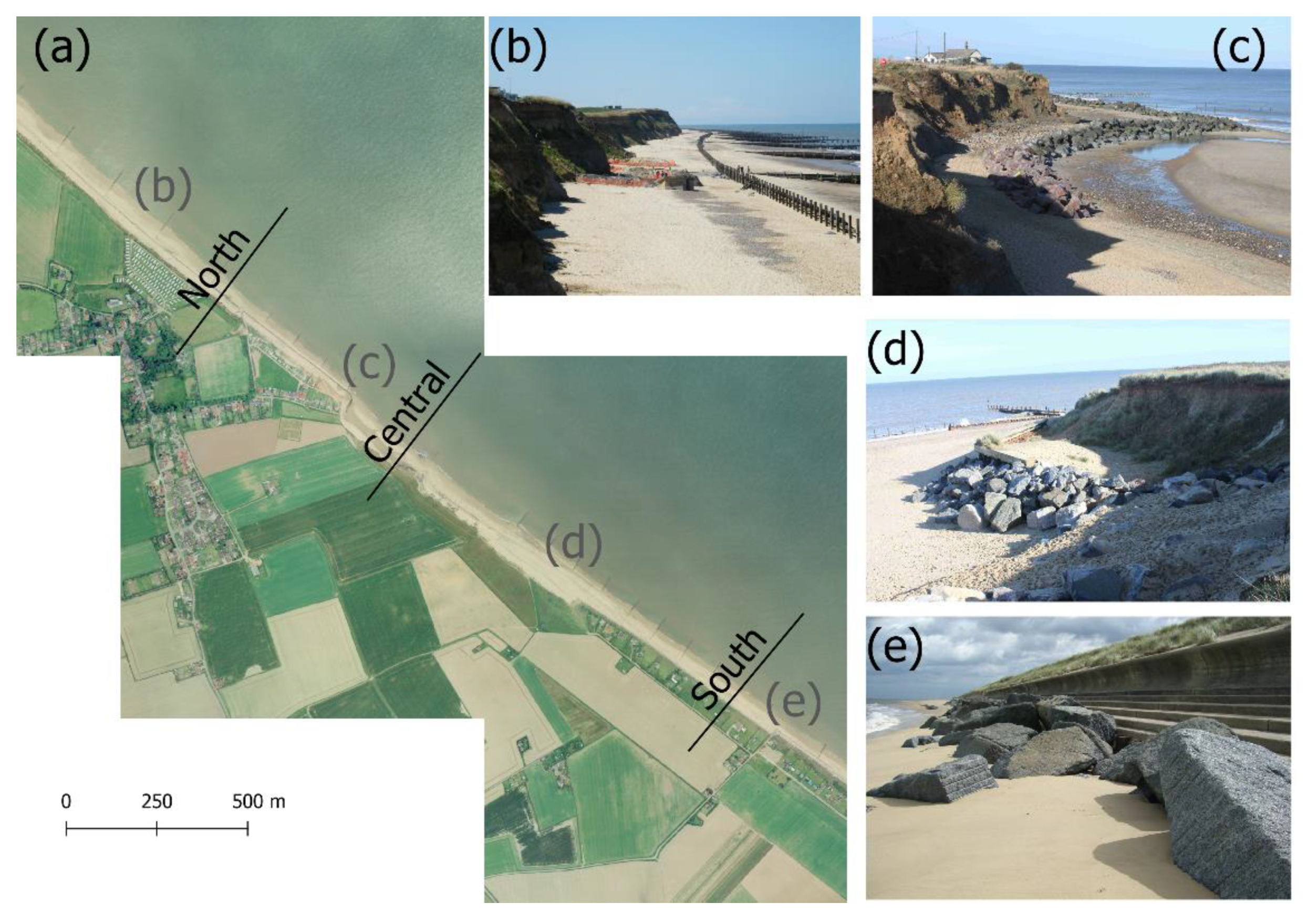
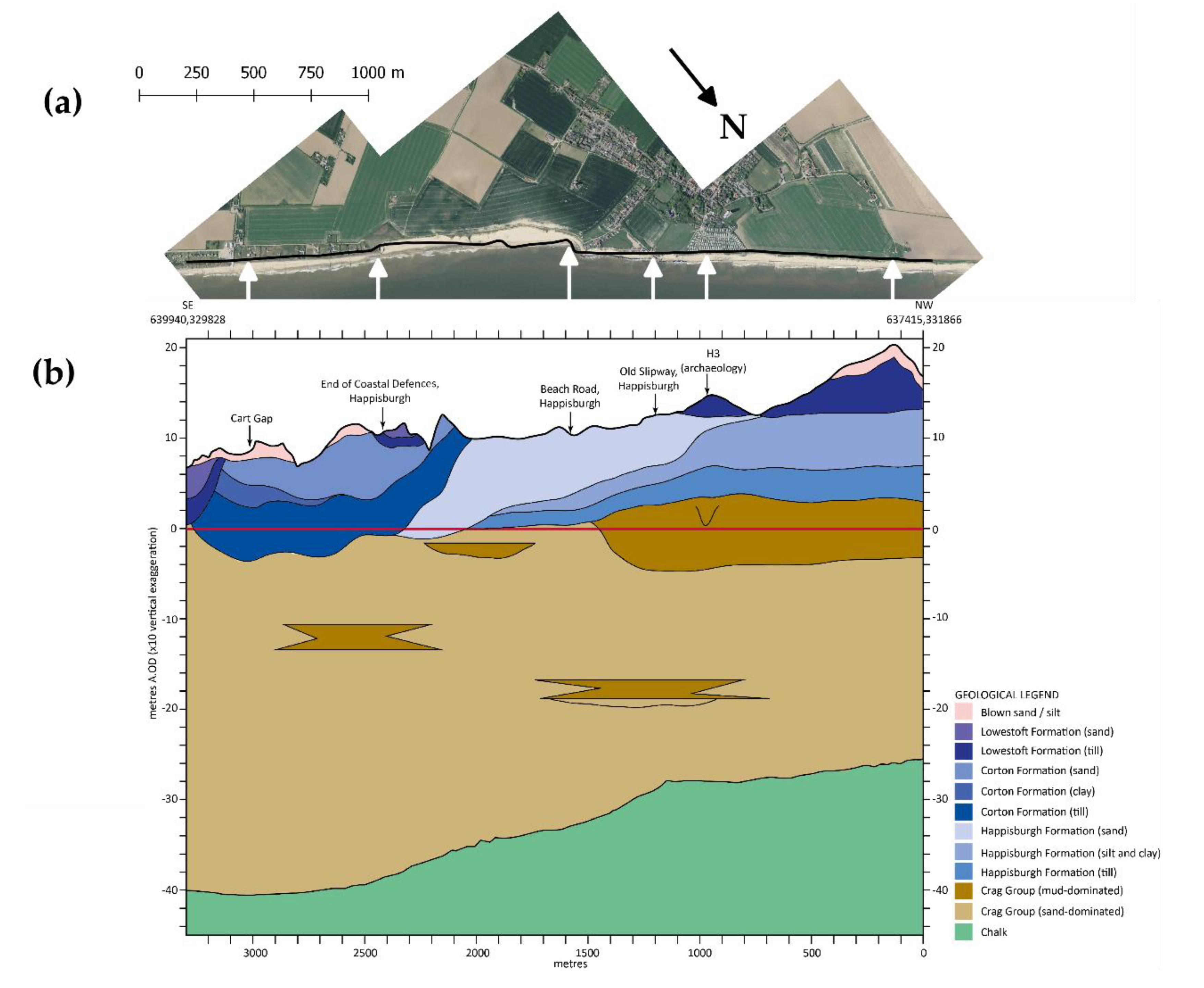
2.1. Happisburgh Case Study Description

Happisburgh is located on the soft sediment coast of Norfolk, eastern England (Figure 2). The length of the coast that is simulated is ca. 3 km. The site is exposed to southern North Sea waves, with average annual significant wave heights (Hs) of 0.9 m and peak periods (Tp) of 4 s from the N-NNE. The wave climate is non-seasonal with similar moderate-energy summers (July to September, Hs = 0.95 m and Tp = 4 s) and moderate-energy winters (October to June, Hs = 0.92 m and Tp = 4 s), and extreme wave heights exceeding Hs = 6 m and Tp = 10 s. The coast is macro-tidal, with a mean spring range of 4.2 m and mean neap range of 2.1 m. Relative sea levels at this location have been rising for millennia, and under natural conditions, this part of the coast is erosional.

Defences were constructed in 1958/59 (wooden revetments and steel sheet piles) and 1968 (wooden groins) [23,24] (Figure 3) on the soft cliff coastline, which formerly eroded at < 1 m/yr [24]. The steel sheet piles are at the landward limit of the groins that lie perpendicular to the coast with a length of 100 m and are spaced along the coast at intervals of 170 m. After construction of the defences, the rate of erosion decreased, and any subsequent loss of land was caused by the failure of unstable cliff slopes. From the late 1980s, the defences were not maintained, in part because of a lack of agreement regarding coastal protection, and in part, because of a lack of funding [23]. By 1991, defence failure led to selective defence removal on safety grounds along 900 m of coast [24], while adjacent defences remained. Subsequently, where defences were removed, excessive retreat occurred and over a period of 14 years, the cliff eroded on average 100 m landward, creating a shallow embayment. Between September 2001 and September 2003, 3.6 × 10⁴ t of sediment was eroded from a 100 m section of the cliff [25] with retreat rates recorded between 8 and 10 m/yr. In 2007, with financial support from the local authority, the local community helped fund rock armouring along the cliff base to slow the erosion [26].

At the southern end of the embayment, a sea-wall protects the low-lying farmland and tourist area of Eccles-on-Sea (Figure 3). This sea-wall was constructed after catastrophic floods in 1953 and in stages up to 1987. There are now three main elements making up the sea defence system: the beach, the sea wall and the sand dunes [27]. The beach becomes highly mobile during storms and can be drawn down to such an extent that the sea wall becomes unstable. In the early and mid-1990s, beaches in the Eccles/Sea Palling area reached critical levels where the sea wall foundations started to fail. Three emergency works contracts were implemented for placing rock protection along the toe of the sea wall. If the sea wall was allowed to collapse, the sand dunes would offer the last line of defence and would be breached rapidly by wave action [27]. Since 1996, the Environment Agency (EA) has undertaken a series of beach nourishments (around 150,000 m³/yr on average [27]) at Sea Palling, about 5 km to the south and down-drift of Happisburgh. This nourishment aims to offset the concomitant reduction in sediment supply from cliff erosion along the Happisburgh-Trimingham coastal section and to maintain sea defence.

The cliffs at the study site have slopes slightly lower than and within the range of their peak angle of friction (i.e., 24 to 32 degrees [28]) and range in height from 6 m to 20 m above Ordnance Datum (OD) (Figure 4). They are composed of a sequence dominated by glacigenic sediments including multiple diamictons (admixtures of poorly-sorted clay, sand and gravel), separated by beds of stratified silt, clay and sand [29,30,31]. These units were deposited during several major incursions of glacier ice into the region during the Middle Pleistocene [32]. The basal unit that crops-out discontinuously at the base of the cliffs is the Crag Group (Early to early Middle Pleistocene age), which is typically obscured by modern beach material but is periodically exposed following storms [25]. The Crag Group consists of stratified sands and clays interpreted as shallow marine to inter-tidal in origin and punctuated by occasional elongated lenticular bodies of fluvial muds [33,34]. The Crag Group rests unconformably on an undulating upper surface of Chalk bedrock (Cretaceous age). Chalk bedrock depths increase from about −25 mOD at the northern end to −40 mOD at the southern end. The large potential stock of sand and gravel at the shore platform present in the Crag Group suggest that the beaches at Happisburgh might not be sediment starved, providing that the waves and currents have enough energy to erode and transport this material towards the coast.

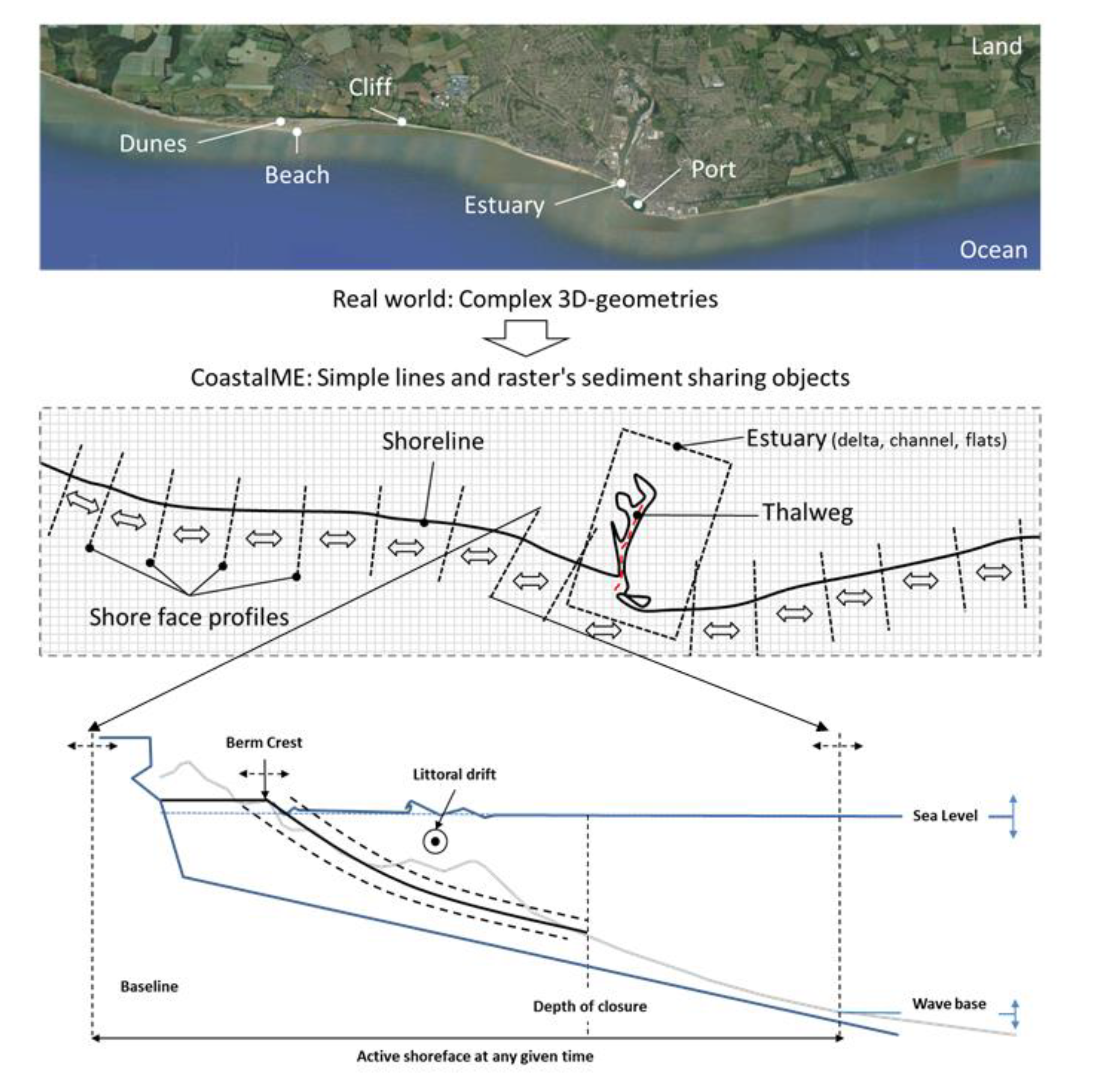
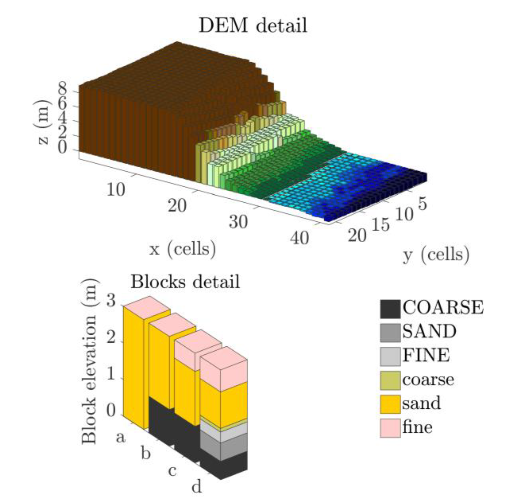
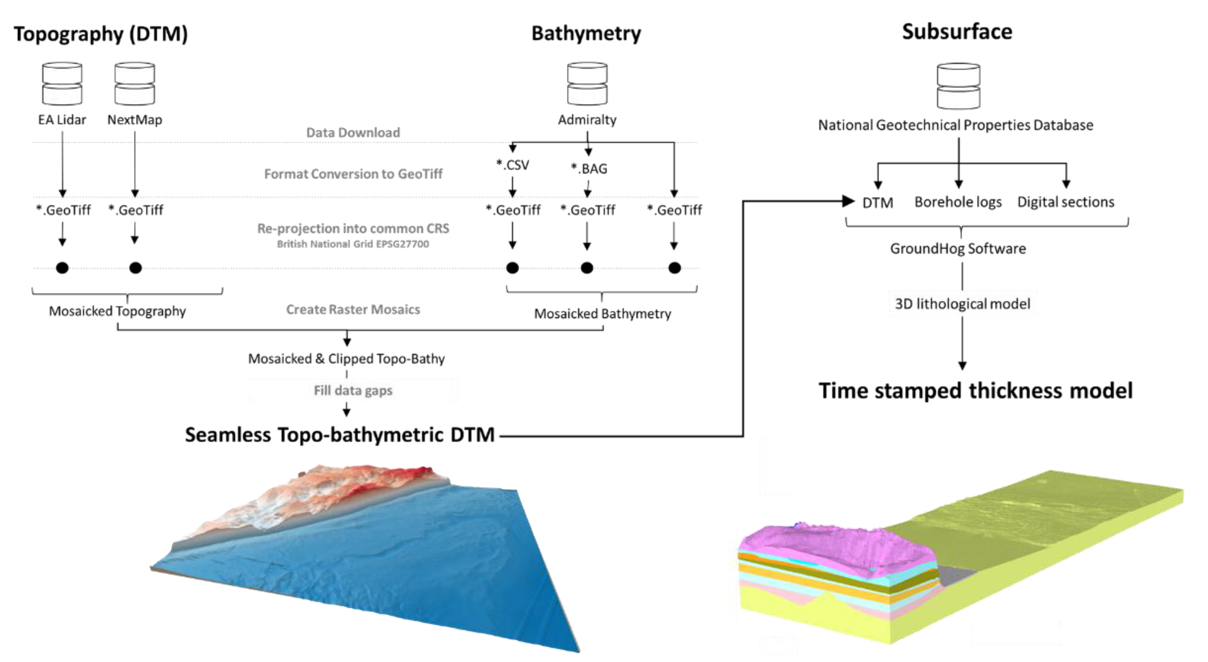
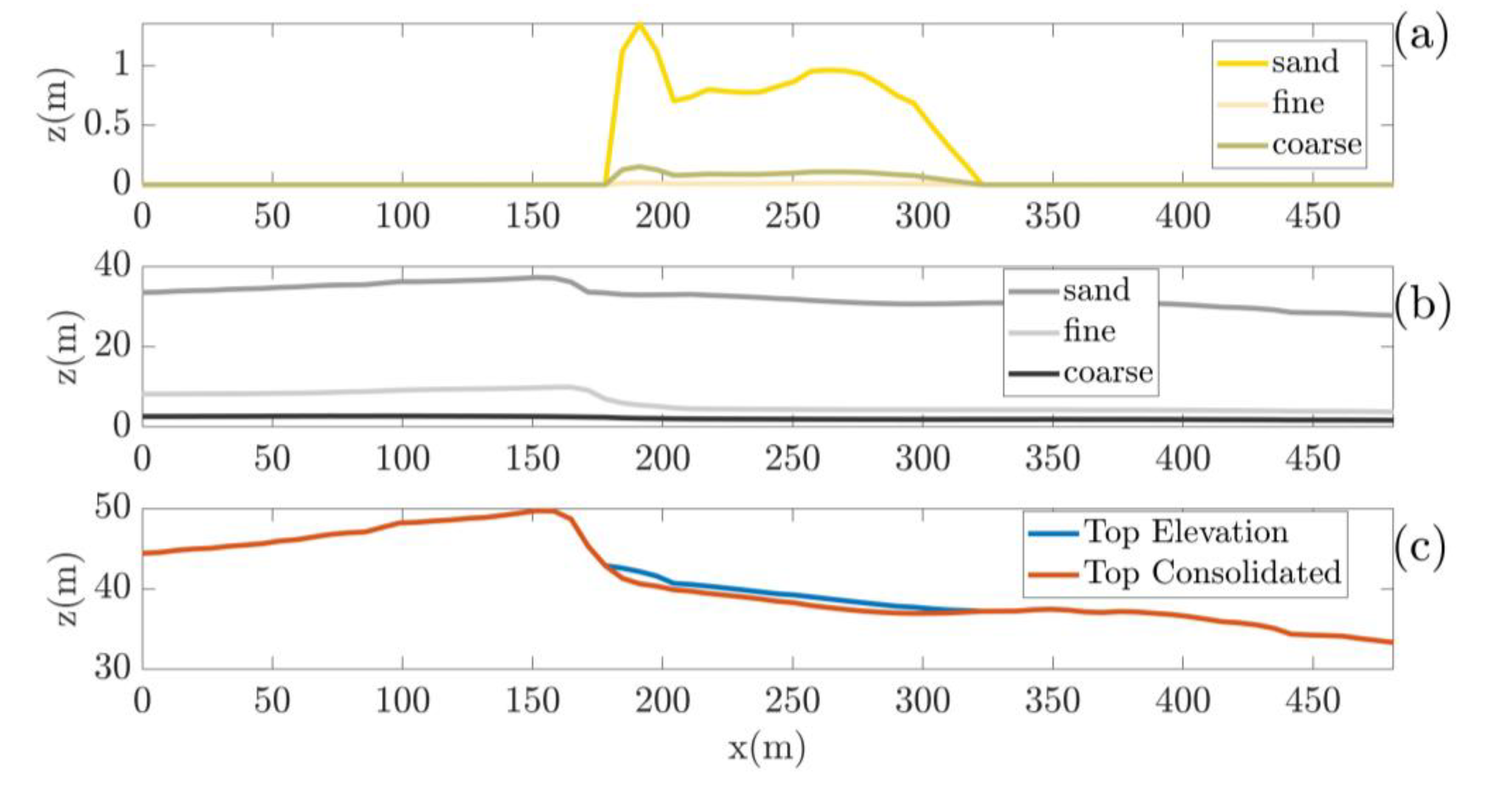
2.2. CoastalME: Concept and Data Structure

CoastalME [35], is a framework to integrate coupled mesoscale reduced complexity models, reductionist coastal area models, data-driven approaches, and qualitative conceptual models. Integration of these heterogeneous approaches gives rise to model compositions that can potentially resolve decadal- to centennial-scale behaviour of diverse coupled open coast, estuary and inner shelf settings. However, coupling existing software models is not a trivial task. One approach involves the coupling of landform specific simulation models (e.g., cliffs, beaches, dunes and estuaries) that have been independently developed [36]. An alternative approach is to capture the essential characteristics of the landform-specific models using a common spatial representation within an appropriate software framework [35]. The latter avoids the problems that result from the model-coupling approach arising from between-model differences in the conceptualisations of geometries, volumes and locations of sediment. CoastalME should be understood as a software framework containing a minimum set of objects and a data structure suitable to integrate any coastal evolution simulation to create a digital model composition (i.e., CoastalME is a tool to create model compositions).

In CoastalME, the shoreface is conceptualised (Figure 5) as a set of sediment sharing cells interconnected by the alongshore sediment transport. Coastal morphological change is simulated as dynamically linked line and raster objects. The hierarchy of panels in Figure 5 illustrates how a real coastal morphology (upper panel) is conceptualised in terms of shoreline, shoreface profiles and estuary elements (middle panel). All elements can share sediment among them (double-headed arrow). The shoreface comprises both consolidated and non-consolidated material that forms the cliff, shore platform and beach, respectively (bottom panel). At every time step, the shoreline is delineated at the intersection of the sea level and the ground elevation. Shore face profiles are defined perpendicular to the shoreline. The sea level and wave energy constrain the proportion of shoreface profiles that are morphologically active at each time step. Eroded sediment from the consolidated profile is added to the drift material to advance the shoreline or loss as suspended sediment. Gradients of the littoral drift further control the advance and retreat of the beach profile and the amount of sediment shared with nearby sections of the coast.

Figure 6 illustrates CoastalME topography and subsurface data structure. Ground elevation is characterised as a set of regular square blocks. The size of the square blocks is determined by the user based on the resolution of data availability and model outputs sensitivity. Each block has a global coordinate x, y, z. Each block might be composed of six different sediment fractions made of coarse sand and fine sediment sizes. Each sediment size fraction can be in a consolidated or unconsolidated state.

Input parameters for CoastalME are supplied via a set of raster, vector, and time series files and a text-format configuration and steering file [37]. Raster files represent the initial ground elevation, sediment thickness and coastal intervention. Vector files specify the locations within the model spatial domain for which wave (wave height, direction and period) forcing time series are provided. Tidal water surface elevation is also provided as a time series input file. CoastalME output consists of GIS layer snapshots, a result summary file, and a number of time-series files. The GIS files include both raster layers such as digital elevation models (DEMs) and sediment thickness and vector layers such as the coastline.

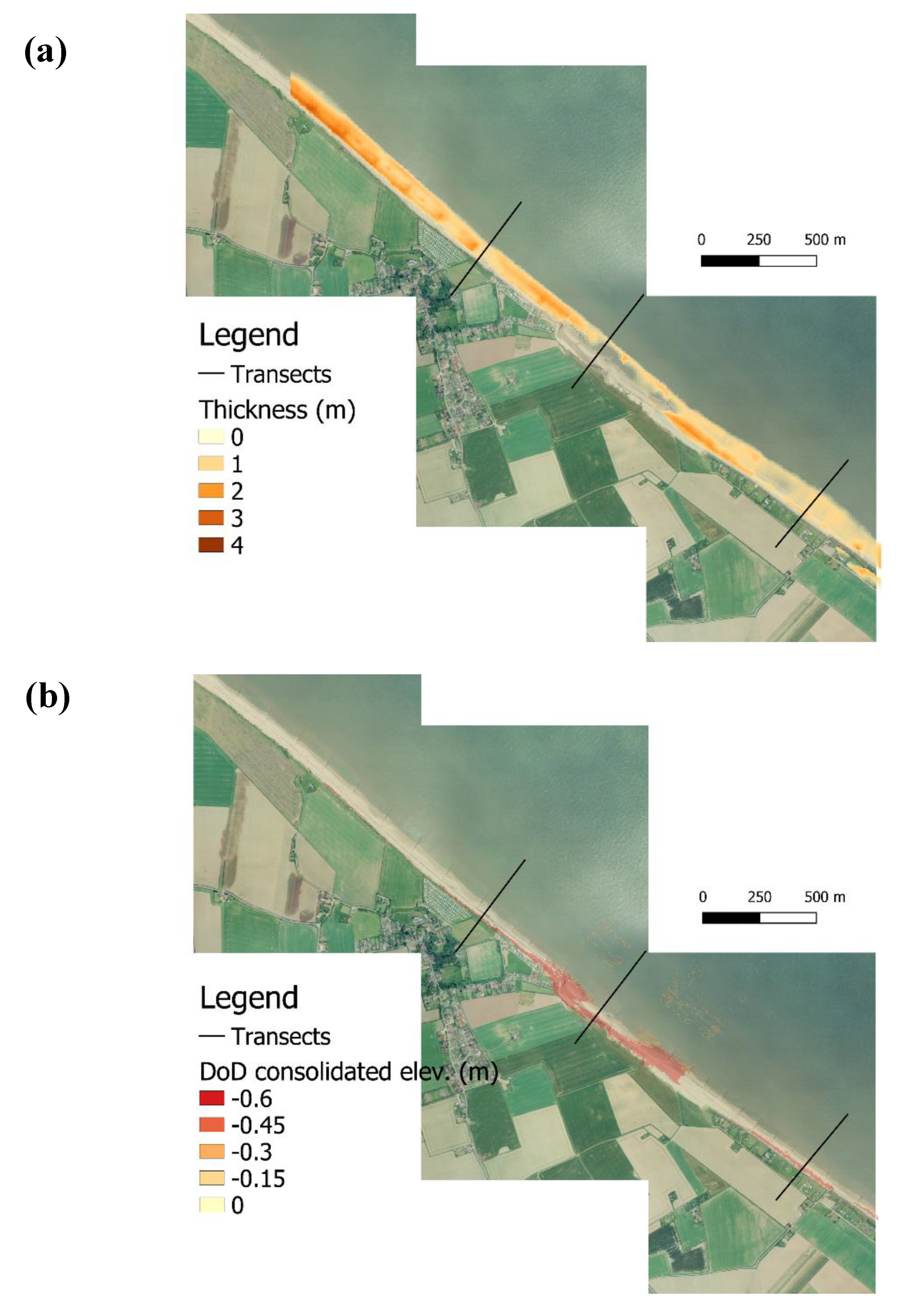
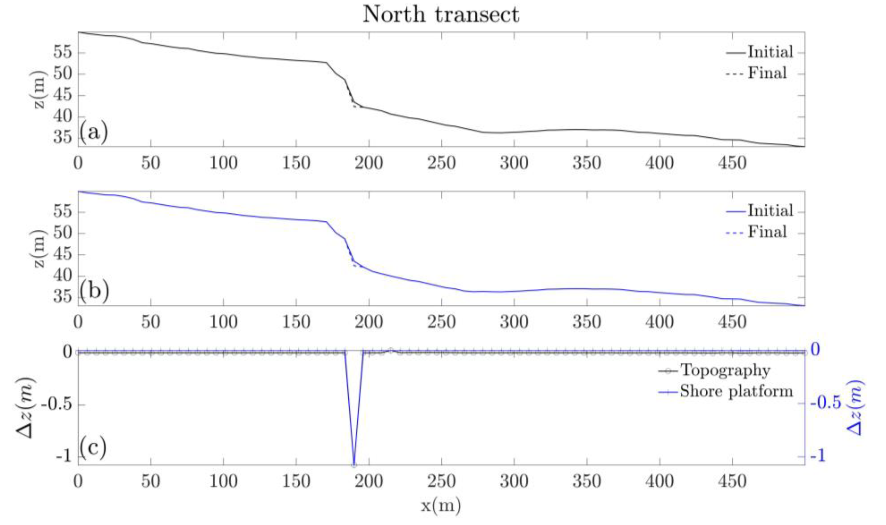
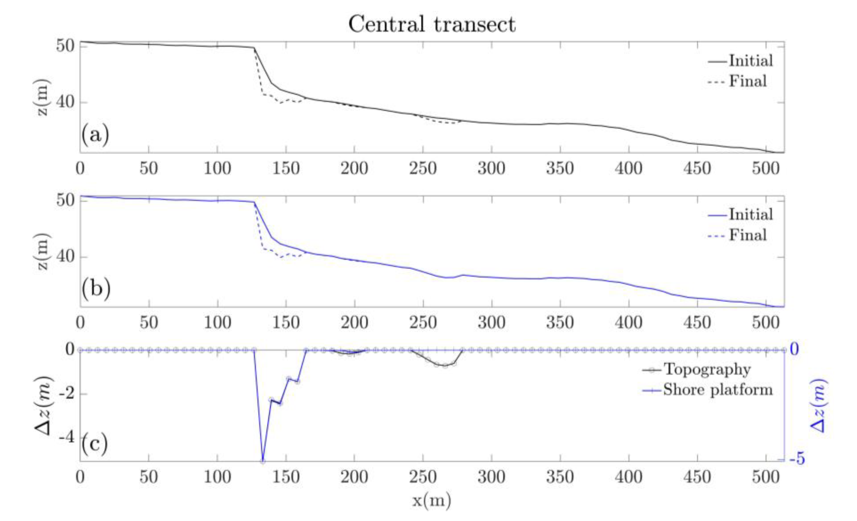
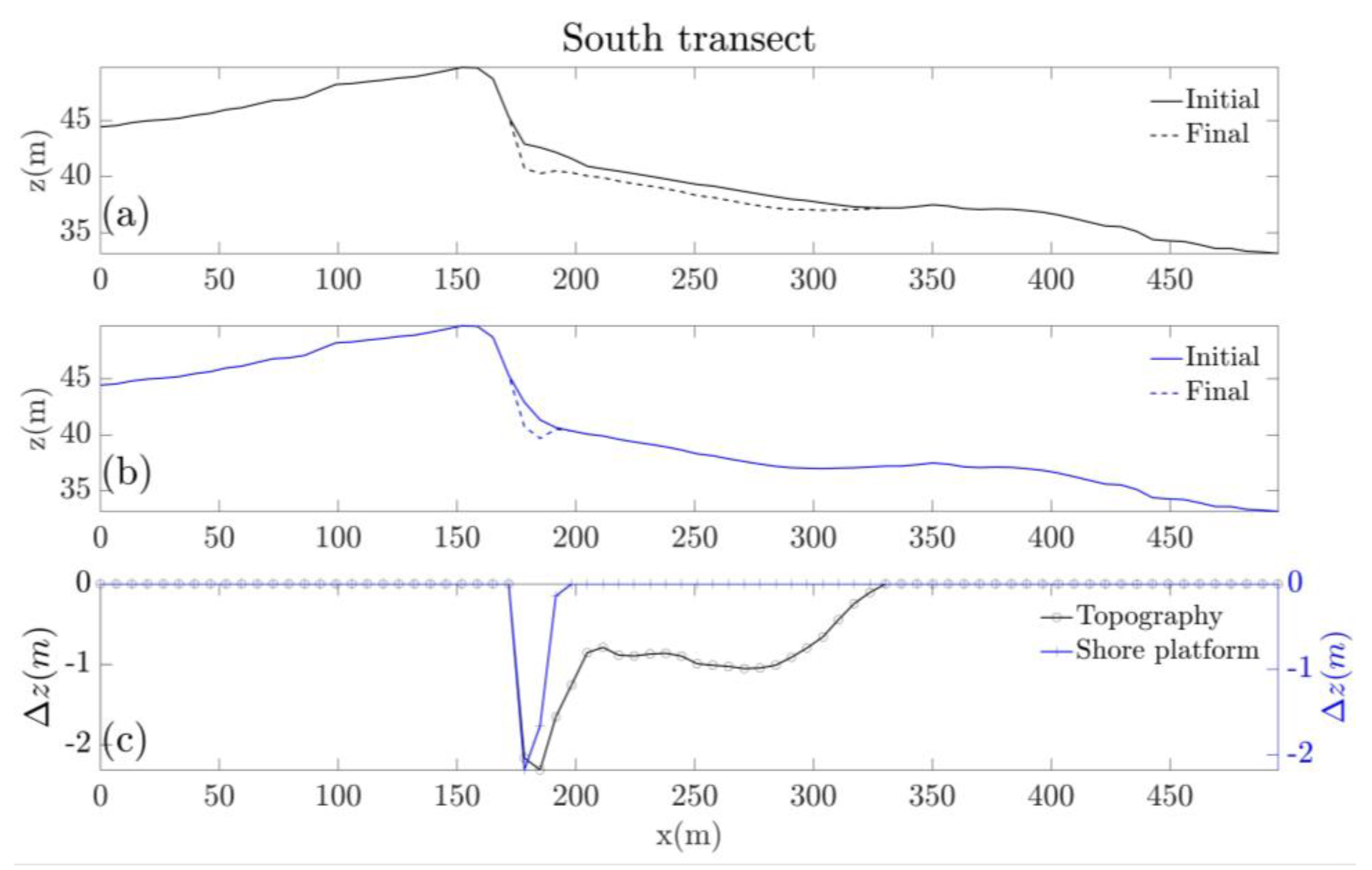
2.3. Simulation Outcomes of Happisburgh Annual Evolution

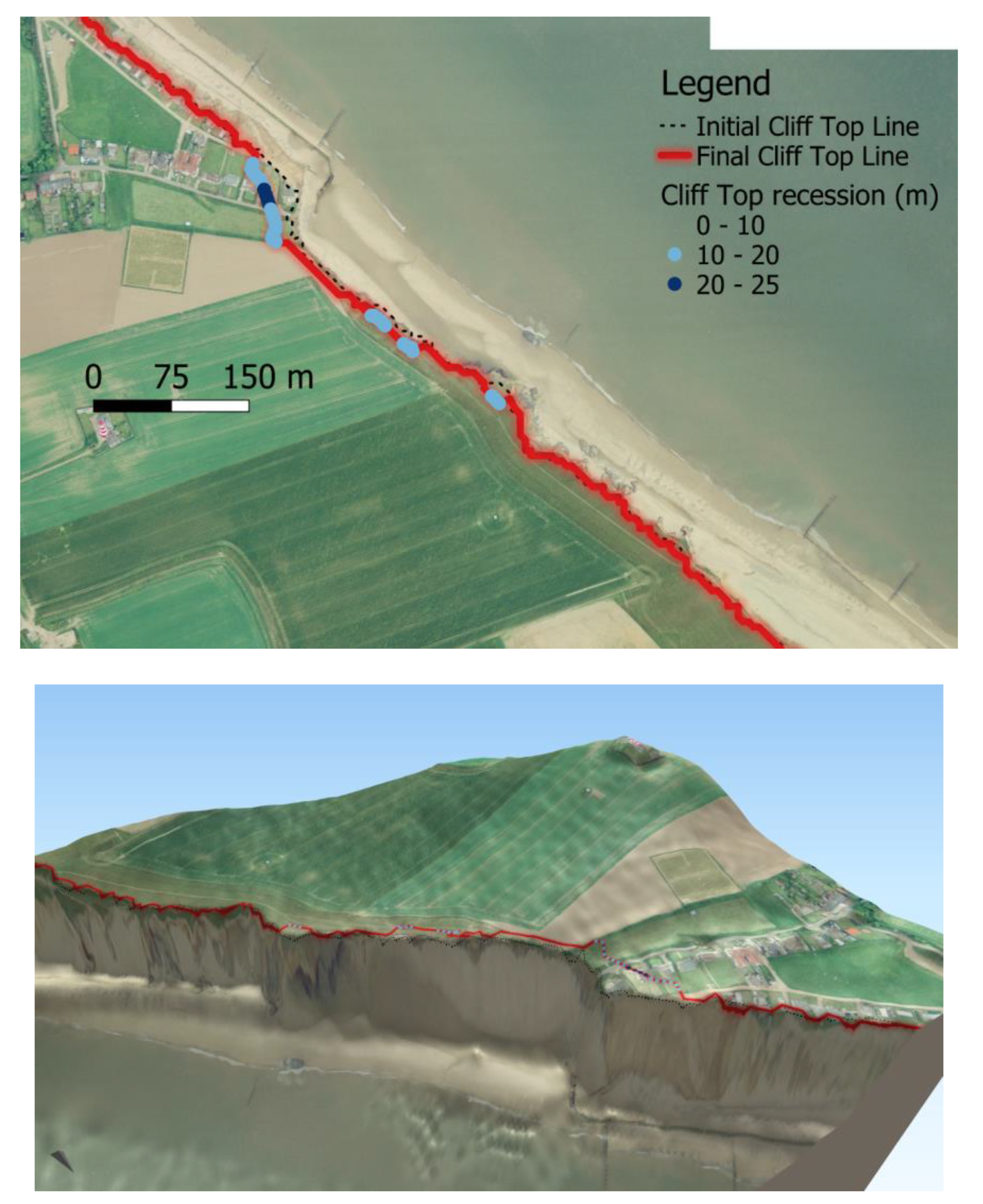
To illustrate the different visualisation options, we have used CoastalME simulation outcomes [19] of the relative contribution of back wearing and down wearing cliff and platform erosion to the near-shore sediment budget under idealised annual forcing conditions at Happisburgh (

Table A1. CoastalME composition model inputs for Happisburgh one year simulation (after [19]).

Input	Value
Required for a generic landscape evolution model
Run duration	360 days
Time step	1 h
Wave heights, direction, period	UKCP09 hindcast data
Topo and bathymetric Digital Elevation Model	LiDAR year 1999 & Multibeam 2011
Tides	Reconstruction of tidal signal using Cromer tide gauge data from 1999 to 2017
Residual elevation	Difference of Cromer tide gauge elevation and tidal levels (gap filled assuming residuals follow a normal distribution)
CoastalME Datum	+40 m above basement level
Coarse, sand and fine sediment content	BGS thickness model
Coarse, sand and fine availability factor	0.3; 0.7; 1.0
Boundary conditions	Open boundaries (i.e., sediment at the boundaries is allotted to exit the grid but no external sediment inputs are assumed over the simulated period)
Required for COVE-sediment sharing module
CERC coefficient	0.79
Length of normal profiles used to create the polygons	800 m
Required for CSHORE-wave propagation module
Breaker ratio parameter γ	0.8
Friction factor fb	0.015
Required for SCAPE-beach & platform interaction
Rock strength and hydrodynamic constant, R	RPlatform = 8 × 104 [m9/4s2/3] RCliff = 8 × 102 [m9/4s2/3]
Beach volume & and beach thickness	Derived from BGS thickness model

Full list of parameters provided in Table S1 in [19].

). This is based on a 360-day simulation at a 1-h numerical time step, with results saved after 1, 30, 60, 90, 120, 150, 180, 210, 230, 260, 290, 310, 340, 360 days. In [19], only the final beach thickness and elevation were shown. For this work, we have used the outcomes obtained for the simulations in best agreement with observations, which were obtained when the rock strength and hydrodynamic constants for the platform and cliff were set equal to 8 × 10⁴ [m^9/4s^2/3] and 8 × 10² [m^9/4s^2/3], respectively. The CoastalME-Happisburgh simulation produced 73 different types of outcomes (

Table A2. CoastalME GIS simulation outcomes name and type. Sorted in filename alphabetical order.

ID	Output name *	Type
1	active_zone	Raster
2	actual_beach_erosion	Raster
3	avg_sea_depth	Raster
4	avg_susp_sed	Raster
5	avg_wave_angle	Vector
6	avg_wave_height	Raster
7	avg_wave_orientation	Raster
8	basement_elevation	Raster
9	beach_change_net	CSV
10	beach_deposition	CSV
11	beach_deposition	Raster
12	beach_erosion	CSV
13	beach_mask	Raster
14	beach_protection	Raster
15	breaking_wave_height	Vector
16	cliff_collapse	Raster
17	cliff_collapse_deposition	CSV
18	cliff_collapse_deposition	Raster
19	cliff_collapse_erosion	CSV
20	cliff_collapse_net	CSV
21	cliff_notch	Vector
22	coast	Vector
23	coast_curvature	Vector
24	cons_sed_coarse_layer_X	Raster
25	cons_sed_fine_layer_X	Raster
26	cons_sed_sand_layer_X	Raster
27	deep_water_wave_angle	Vector
28	deep_water_wave_height	Raster
29	deep_water_wave_orientation	Raster
30	downdrift_boundary	Vector
31	ErosionPotential	CSV
32	intervention_class	Raster
33	intervention_height	Raster
34	invalid_normals	Vector
35	landform_class	TIF
36	local_cons_sediment_slope	Raster
37	mean_wave_energy	Vector
38	node	Vector
39	normals	Vector
40	platform_erosion	CSV
41	polygon	Vector
42	polygon_gain_or_loss	Raster
43	polygon_raster	Raster
44	polygon_updrift_or_downdrift	Raster
45	potential_beach_erosion	Raster
46	potential_platform_erosion	Raster
47	rcoast	Raster
48	rcoast_normal	Raster
49	sea_area	CSV
50	sea_depth	Raster
51	sediment_top_elevation	Raster
52	shadow_boundary	Vector
53	shadow_downdrift_zones	Raster
54	shadow_zones	Raster
55	still_water_level	CSV
56	susp_sed	Raster
57	suspended_sediment	CSV
58	top_elevation	Raster
59	total_actual_beach_erosion	Raster
60	total_actual_platform_erosion	Raster
61	total_beach_deposition	Raster
62	total_cliff_collapse	Raster
63	total_cliff_collapse_deposition	Raster
64	total_potential_beach_erosion	Raster
65	total_potential_platform_erosion	Raster
66	uncons_sed_coarse_layer_X	Raster
67	uncons_sed_fine_layer_X	Raster
68	uncons_sed_sand_layer_X	Raster
69	wave_angle	Vector
70	wave_energy	Vector
71	wave_height	Raster
72	wave_orientation	Raster
73	wave_period	Raster

* The output file name is completed by a four digit number indicating the time interval (i.e., wave_period_0001 is the output for interval 1).

), which includes 11 Comma Separated Value (CSV) files, 14 GIS vector files and 48 GIS raster files. The raster and vector files are snap-shots at user-defined intervals, while CSV files contain time series for all time-steps (here 86,400 representing 360 days at a 1-h interval).

Figure 7 illustrates the overall workflow followed by [19] to obtain the thickness model used for the idealised Happisburgh simulation. Payo et al. [16] first generated a 3D thickness model using three data sets (topography, bathymetry and subsurface lithology, using existing databases) as required by the CoastalME data structure, although, the proposed workflow is transferable to any other place where equivalent data sets are available. Firstly, the topography and bathymetry database are combined to create a seamless topo-bathymetric Digital Terrain Model (DTM) of the study site. For Happisburgh, this combined Environment Agency LIDAR DTM data for 1999 for the inland topography and multibeam bathymetry for 2011. The composite data set has some gaps along the coast, where water depth is too shallow for the vessels operating the multibeam to obtain good quality data but still beyond the reach of the LIDAR. A seamless topo-bathymetric-DTM was produced by interpolation after resampling to a 5 m grid. For the interpolation, we used the SAGA-Close Gaps function with a tension threshold of 0.1. The Close Gaps function uses a method commonly called minimum curvature under tension to interpolate missing data [38]. This DTM is then combined with the subsurface database to produce, first, a 3D geological model of the Quaternary sediments and, second, a thickness model. The 3D geological model was generated by combining the DTM, surface geological line-work and downhole borehole and geophysical data to enable the geologist to construct cross-sections by correlating boreholes and the outcrops to produce a geological fence diagram. Interpolation between the nodes along the drawn sections and the limits of the units produces a solid model comprising a stack of triangulated objects each corresponding to one of the geological units present. For the interpolation of the 3D geological model, we used GSI3D^TM software (Keyworth, UK, version 2013) [39] as described in [19]. Then, the elevation of the top and base of each geological unit (i.e., its thickness) is calculated by triangulating between digitized nodes along the cross-sections and nodes around the edges of unit coverages. These tops, bases and thicknesses are then exported from the model as grids with a user-defined cell size. Using empirical knowledge, supported by data from the BGS National Geotechnical Database [40], the litho-stratigraphical units expressed in the model were assigned average percentages for fines (<0.63 mm), sand (0.63–2 mm) and coarse material (>2 mm) (Table A1 [19]). The chalk consists mainly of silt particles and, although it forms a consolidated rock, was added to the fines fraction. All organic material was also assigned to the fines fraction. The geological model was queried to calculate the average grain size distribution of the geological sequence at each node of a 5 × 5 m grid. The resulting data were converted into raster thickness layers.

3. Results

Figure 8 shows the different sediment fractions along the Happisburgh South transect for both the unconsolidated material (e.g., beach deposits) and consolidated platform. The sediment fractions (coarse, fine and sand) shown have been extracted from the raster outputs numbers 24, 25, 26 on Table A2 for the consolidated material and outputs numbers 66, 67 and 68 for the unconsolidated material at t = 1 day. QGIS (v 3.10.2) and the Profile-Tool (v 4.1.7) plugin were used to extract elevations along the transect. Figure 8a shows the sediment fractions (as thicknesses) for the unconsolidated material, which for Happisburgh represents the beach material. Given that the 3D grid is constructed at a 5 m interval, a thickness of 1 m is equivalent to 25 m³ of material per spatial cell. For this transect, the beach deposit is dominated by sand with a relatively uniform thickness of 0.8 m along the beach (and a maximum of 1.34 m). The equivalent thickness of coarse material is an order of magnitude less (about 0.08 m with a maximum of 0.15 m). Fine material is negligible (<0.01 m). The unconsolidated material is also dominated by the sand fraction with a maximum thickness of 37 m, followed the fine fraction (maximum thickness of 10 m) and coarse material (always < 2.7 m). By adding together all fractions for the consolidated and unconsolidated material, we obtain the top elevation of the consolidated platform and actual topographic elevation, respectively (Figure 8c).

Figure 9a shows the beach deposit thickness, obtained from the difference between the topographic elevation and the consolidated platform top elevation, overlaid on an aerial image. Beach deposit thickness varies across and along the shoreline, ranging from 4 m in the north, minimal to non-existent along the undefended central section, and 2–3 m in the southern sector. As expected, the simulated lowering of the consolidated platform (Figure 9b) is largest at places where the beach deposits thickness is least and cannot offer protection. These differences in beach thickness, combined with the different defence structures close to each transect, have an appreciable effect on the simulated elevation changes (Figure 10, Figure 11 and Figure 12).

Figure 10 shows the elevation change of the topographic elevation and consolidated elevation along the North transect computed for the 360-day run. The overall topographic elevation (Figure 10a) has been obtained by adding together all fractions for the consolidated and unconsolidated material of the raster files numbers 24, 25, 26 and 66, 67, 68 on Table A2. The top elevation of the consolidated platform (Figure 10b) has been obtained by adding all fractions of the consolidated material (i.e., outputs 24, 25, 26 on Table A2). On the North transect, where beach thickness is low (0–1 m) the topographic elevation and the upper elevation of the consolidated platform coincide. This section of coast is protected by sheet piling, which significantly reduces the erosion behind the defences. As expected, the simulated elevation change is concentrated at the toe of the cliff, which retreats 6 m landward over the year. Elevation decreases along the entire profile (i.e., no accretion occurs) with a maximum vertical erosion of 1 m.

Figure 11 shows the elevation change of the top total elevation and consolidated elevation along the Central transect. As with the North transect, where beach thickness is low (0–1 m), the topographic elevation coincides with the top of the consolidated material. As expected for this undefended stretch of coast, cliff toe retreat and vertical erosion are more rapid than that simulated for the defended North and South transects. Cliff toe retreat is approximately 33 m and vertical erosion is up to 5 m. The beach deposit is decreased by a maximum of 0.7 m but remains thick enough to protect the consolidated platform underneath, the elevation of which remains unchanged.

Figure 12 shows the equivalent results along the South transect, where the beach thickness is greater (1–2 m). Cliff toe horizontal location remains unchanged because this section is protected by a sea-wall. Topographic lowering is no longer restricted to the proximity of the cliff toe and is appreciable, with an average value of −0.8 m, along the entire active transect with a maximum vertical erosion of −2 m close to the sea-wall toe. However, lowering of the consolidated platform is still constrained to the region nearby the sea-wall toe where it reaches a maximum of 2 m. This implies that the topographic lowering is mostly due to vertical erosion of the consolidated platform near the sea-wall toe while, seawards, the lowering is due to beach material being lost due to longshore sediment transport gradient. Even here, the beach appears to remain thick enough to protect the underlying consolidated platform from lowering.

Figure 13 shows the initial and final simulated cliff top lines along with a Digital Elevation Model (DEM) created from the topographic elevation. Cliff top lines were extracted using the CliffMetric automatic delineation algorithm proposed by Payo et al. (2015). Cliff top and toe location points have been converted into lines and the shortest distance between the final and initial cliff top points used as an indication of cliff retreat. A maximum cliff top retreat of 30 m is obtained in the north of the non-defended coastal section, while the cliff top remains unchanged (i.e., differences smaller than one diagonal cell length or 7 m) for the defended sections. The lines are plotted on a 2D view of the study area and 3D view with aerial imagery as background to facilitate geolocation.

4. Discussion

The credibility of any simulation of mesoscale coastal geomorphological change, for both specialist and non-specialists, depend on three essentials: (1) Data—the quality of the data on which the simulation model is based; (2) Model—the fidelity of the algorithms, the validity of the assumptions and the correctness of the underlying computer code; and (3) Visualisation—representation of model outputs that can be clearly linked to the underlying model prediction and the real-world problem. These aspects are considered further here in relation to the Happisburgh case.

Regarding the quality of the data, we have shown how the Happisburgh study zone can be represented using the CoastalME data structure (Figure 6) by combining existing digital elevation and sub-surface data (Figure 7) to initialise a 3D thickness model. This 3D thickness model is based on different types of data (LiDAR-DTM + Multibeam bathymetry + borehole logs and cross-shore sections of the subsurface) and the steps required to combine this variable set of data types are transparent and reproducible. In particular, the discrete nature of the databases (i.e., boreholes logs and cross-sections) and the data gap of bathymetry in the very shallow nearshore region and offshore region can be filled-in using different interpolation approaches. Combining these three databases allows a better representation of the supply of transportable material, which is essential to obtain an accurate estimate of the nearshore sediment balance and ultimately the coastal morphological change. The amount of transportable material can be visualised in a number of ways; as thicknessses of different sediment fractions along selected transects (Figure 8) or as a raster map of beach thickness (Figure 9).

The fidelity of the algorithms included in the CoastalME model composition used for the Happisburgh digital model was discussed in detail by [19]. They showed that the main features (i.e., cliff, beach, shore-platform, sea-wall, and palisade) and its interaction were incorporated in the model composition (i.e., structural validity). Here, we have illustrated the validity of the assumptions and the competence of the code by showing how the digital model forced with a one-year simulation of wave and tidal forcing shows a rich and plausible behaviour as supported from field data [20] and expected for an eroding soft coastline with defended and non-defended coastal stretches (Figure 10, Figure 11 and Figure 12). Furthermore, the simulation outputs also provide insights of a potentially significant platform down-wearing in-front of the sea-wall that is very difficult to observe in the real system since the platform in-front of the sea-wall is often covered by the beach, precluding direct observation of the lowering (Figure 9).

We have shown how model outputs can be clearly linked to the underlying model prediction as 1D, 2D and 3D geo-indicators. Contrary to the loose linkage presented by [12] where 1D model outputs were translated into 3D-DEM during the visualisation stage, we have shown here how the CoastalME model output “sediment_top_elevation”, representing the top total sediment elevation, is effectively a georeferenced evolving 3D-DEM. This sidesteps the need for further assumptions during the visualisation stage (i.e., cliff toe line being parallel to cliff top line as done by [12]) that might not be always scientifically justified. We have shown how other 1D and 2D geo-indicators of change used by specialist and non-specialist [41] such as sediment fraction composition (Figure 8), elevation profile (Figure 10, Figure 11 and Figure 12), and cliff top line (Figure 13) can be extracted from the evolving 3D-DEM. CoastalME uses the georeferenced system used for the 3D-thickness input model as the default reference system for all the vector and raster outputs (Table A2), which makes it very straightforward to combine the model outputs with other georeferenced information that facilitates communication of the outputs. For example, we have shown how the outputs can be combined in 2D and 3D with aerial imagery, and vector lines (Figure 13).

We acknowledge several key limitations that presently hinder the more widespread use of the proposed methodology (Figure 7) to create digital representation at other locations throughout the UK. In no particular order, these limitations are;

• Lack of a national coastal defence database. The Environment Agency’s Asset Information Management System contains the location of flood defences owned, managed or inspected by the EA and coastal protection assets managed by other operating authorities. Data includes defence type (i.e., groin, sheet pile, palisade, etc.) location and main dimensions as designed and may include a condition grade from an asset inspection [42]. However, not all attributes are present. Additionally, private defensive structures are excluded. This lack of data makes it very difficult to ensure that the coastal interventions represented in the model correspond with the coastal defence on the ground. For the example of Happisburgh presented here, the depth of the sheet piles is unknown making it impossible to assess the risk of scouring undermining the sheet pile and consequent ultimate failure.
• Need for more frequently updated topo-bathymetric databases. The coastal topography and bathymetry is dynamic and continuously changing over time. The EA-LiDAR DTM and UKHO multi-beam bathymetries have good spatial coverage but provide only snap-shots at given dates of the state of the physical system. As the different agencies in charge of updating the DTMs operate independently and with different budgets, the date of the most up to date DTM available might vary from place to place. While daily updates of the topo-bathymetry DTM are unlikely to be needed for the purpose of exploring “what if” scenarios at decadal and longer time scales, they are extremely valuable for ongoing model validation.
• Sensitivity of simulation outputs to interpolations and modeller assumptions. Due to the discrete nature of geotechnical data and the existence of gaps in topographic and bathymetric data, interpolation will likely remain an important part of any simulation model. The choice of model resolution (spatial and temporal) is one of the many decisions that can affect the simulation of sub-mesoscale scale features. Sub-grid features (and processes) are necessarily smoothed out by interpolation onto coarser grids, and this may influence the depiction and prediction of mesoscale morphological change. Although it has been argued [43,44] that mesoscale coastal morphodynamics is substantially decoupled from small-scale processes, this is clearly an aspect of model development that requires careful attention. Sensitivity testing of the overall simulation outputs to different interpolation, resolution and other model assumptions ideally require a standardised approach.
• The need for a curator of model composition and model instances. To realise maximum benefit from the resource investment in environmental/earth science models, it is necessary to record a rich set of model metadata. This metadata should include attributes such as which environmental/earth science discipline is involved, and which parameters are input and output in the modelling process. In 2016, NERC created the Model Metadata Application (http://model-search.nerc.ac.uk/) to help users discover and locate the existence of models, and also descriptive or "usage" metadata which is of relevance when making use of a model, for example, when using a model code developed by another researcher. As coastal model compositions and coastal model instances become available in the future, they will need to be recorded accordingly in the Model Metadata Application or any similar platform.

5. Conclusions

It has been recognised by [12] that by linking an erosion model with a GIS and then developing the resulting spatial information into visualisations of the evolving coastal environment, information on the changing hazard of future coastal recession can be made more accessible to non-specialists. Non-specialists generally seem to welcome the additional detail and realism that the visualisations provide, and acknowledge the communication and awareness-raising value of the images. The credibility of the resulting virtual future landscapes is also enhanced by their derivation from scientific data provided by specialists using simulation models. A key issue that emerges is that the quest for realism in visualisation can lead to more detailed data demands than can be provided by the underlying scientific model supplying the rationale for the landscape predictions.

In this work we have attempted to address a knowledge gap concerning the important but still unexplored challenge of communicating simulations of mesoscale coastal dynamic evolution to specialist and non-specialist audiences. We have shown how the risk of simulation model outcomes becoming loosely connected to more realistic visualisations of model outcomes can be minimised by using the Coastal Modelling Environment framework. CoastalME is a bespoke modelling framework for coastal mesoscale morphological modelling with close linkages between the scientific model abstractions, in the form of lines, areas and volumes, the 3D representation of the coastal topo-bathymetry elevation and shallow sub-surface sediment fraction composition. We have proposed and illustrated through the study case of Happisburgh, East England (UK), a transparent and reproducible methodology to merge the required variety of data types and formats into a 3D-thickness model that is used to initialise the simulation. We also highlight some of the limitations that are preventing the direct adoption of the methodology proposed.

References

1. French, J.R.; Burningham, H. Coastal geomorphology: Trends and challenges. Prog. Phys. Geogr. Earth Environ. 2009, 33, 117–129. [Google Scholar] [CrossRef]
2. French, J.; Payo, A.; Murray, B.; Orford, J.; Eliot, M.; Cowell, P. Appropriate complexity for the prediction of coastal and estuarine geomorphic behaviour at decadal to centennial scales. Geomorphology 2016, 256, 3–16. [Google Scholar] [CrossRef] [Green Version]
3. Kamphuis, J. Beyond the limits of coastal engineering. In Coastal Engineering 2006; World Scientific: Singapore, 2007; Volumes 5, pp. 1938–1950. [Google Scholar]
4. Hanson, H.; Aarninkhof, S.; Capobianco, M.; Jimenez, J.; Larson, M.; Nicholls, R.; Plant, N.; Southgate, H.; Steetzel, H.; Stive, M. Modelling of coastal evolution on yearly to decadal time scales. J. Coast. Res. 2003, 19, 790–811. [Google Scholar]
5. Bray, M.; Hooke, J.; Carter, D. Planning for sea-level rise on the south coast of england: Advising the decision-makers. Trans. Inst. Br. Geogr. 1997, 22, 13–30. [Google Scholar]
6. Green, D.R. The role of public participatory geographical information systems (PPGIS) in coastal decision-making processes: An example from Scotland, UK. Ocean Coast. Manag. 2010, 53, 816–821. [Google Scholar] [CrossRef]
7. Blunkell, C.T. Local participation in coastal adaptation decisions in the UK: Between promise and reality. Local Environ. 2017, 22, 492–507. [Google Scholar] [CrossRef]
8. Robinson, S. Conceptual modelling for simulation part II: A framework for conceptual modelling. J. Oper. Res. Soc. 2008, 59, 291–304. [Google Scholar] [CrossRef]
9. French, J.; Burningham, H.; Thornhill, G.; Whitehouse, R.; Nicholls, R.J. Conceptualising and mapping coupled estuary, coast and inner shelf sediment systems. Geomorphology 2016, 256, 17–35. [Google Scholar] [CrossRef] [Green Version]
10. Payo, A.; Hall, J.W.; French, J.; Sutherland, J.; van Maanen, B.; Nicholls, R.J.; Reeve, D.E. Causal loop analysis of coastal geomorphological systems. Geomorphology 2016, 256, 36–48. [Google Scholar] [CrossRef] [Green Version]
11. Forrester, J.W.; Senge, P.M. Tests for Building Confidence in System Dynamics Models; System Dynamics Group, Sloan School of Management, Massachusetts Institute of Technology Cambridge: Cambridge, MA, USA, 1978. [Google Scholar]
12. Brown, I.; Jude, S.; Koukoulas, S.; Nicholls, R.; Dickson, M.; Walkden, M. Dynamic simulation and visualisation of coastal erosion. Comput. Environ. Urban Syst. 2006, 30, 840–860. [Google Scholar] [CrossRef]
13. Appleton, K.; Lovett, A. Gis-based visualisation of rural landscapes: Defining ‘sufficient’realism for environmental decision-making. Landsc. Urban Plan. 2003, 65, 117–131. [Google Scholar] [CrossRef]
14. Cowell, P.J.; Roy, P.S.; Jones, R.A. Shoreface translation model: Computer simulation of coastal-sand-body response to sea level rise. Math. Comput. Simul. 1992, 33, 603–608. [Google Scholar] [CrossRef]
15. Walkden, M.J.; Hall, J.W. A mesoscale predictive model of the evolution and management of a soft-rock coast. J. Coast. Res. 2011, 27, 529–543. [Google Scholar] [CrossRef]
16. James, J.; Region, A.; House, K.; Way, G.; Goldhay, O. Sediment input from coastal cliff erosion. Br. Geol. Surv. 1995, 74. (TR/577/4/A). [Google Scholar]
17. Dickson, M.E.; Walkden, M.J.A.; Hall, J.W. Systemic impacts of climate change on an eroding coastal region over the twenty-first century. Clim. Chang. 2007, 84, 141–166. [Google Scholar] [CrossRef]
18. Walkden, M. Scape Modelling of Shore Evolution: Cromer to Cart Gap, Appendix C of the Cromer to Winterton Ness Coastal Management Study; Royal Haskoning Report for Mott Macdonald, on behalf of North Norfolk District Council: Penryn, UK, July 2013. [Google Scholar]
19. Payo, A.; Walkden, M.; Ellis, M.; Barkwith, A.; Favis-Mortlock, D.; Kessler, H.; Wood, B.; Burke, H.; Lee, J. A quantitative assessment of the annual contribution of platform downwearing to beach sediment budget: Happisburgh, England, UK. J. Mar. Sci. Eng. 2018, 6, 113. [Google Scholar] [CrossRef] [Green Version]
20. López, P.M.; Payo, A.; Ellis, M.A.; Criado-Aldeanueva, F.; Jenkins, G.O. A method to extract measurable indicators of coastal cliff erosion from topographical cliff and beach profiles: Application to North Norfolk and suffolk, East England, UK. J. Mar. Sci. Eng. 2020, 8, 20. [Google Scholar]
21. Payo, A.; Walkden, M.; Barkwith, A.; Ellis, A.M. Modelling rapid coastal catch-up after defence removal along the soft cliff coast of Happisburgh, UK. In Proceedings of the 36th International Conference on Coastal Engineering, Baltimore, MD, USA, 30 July–3 August 2018; ASCE: Baltimore, MD, USA; p. 2. [Google Scholar]
22. Walkden, M.; Watson, G.; Johnson, A.; Heron, E.; Tarrant, O. Coastal Catch-Up Following Defence Removal at Happisburgh; Coastal Management, ICE: London, UK, 2016; pp. 523–532. [Google Scholar]
23. Brown, S.; Barton, M.E.; Nicholls, R.J. Shoreline response of eroding soft cliffs due to hard defences. In Proceedings of the Institution of Civil Engineers-Maritime Engineering; Thomas Telford Ltd.: London, UK, 2014; Volume 167, pp. 3–14. [Google Scholar]
24. Clayton, K.M. Sediment input from the norfolk cliffs, Eastern England—A century of coast protection and its effect. J. Coast. Res. 1989, 5, 433–442. [Google Scholar]
25. Poulton, C.V.; Lee, J.; Hobbs, P.; Jones, L.; Hall, M. Preliminary investigation into monitoring coastal erosion using terrestrial laser scanning: Case study at happisburgh, norfolk. Bull. Geol. Soc. Norfolk 2006, 56, 45–64. [Google Scholar]
26. Frew, P. Adapting to coastal change in North Norfolk, UK. In Proceedings of the Institution of Civil Engineers-Maritime Engineering; Thomas Telford Ltd.: London, UK, 2012; Volume 165, pp. 131–138. [Google Scholar]
27. Hayman, S. Eccles to Winterton on Sea Coastal Defences; SH/RG BF190712; Environment Agency, Norfolk Broads Forum: Norfolk, UK, 2012; p. 3. [Google Scholar]
28. Hobbs, P.; Pennington, C.; Pearson, S.; Jones, L.; Foster, C.; Lee, J.; Gibson, A. Slope Dynamics Project Report: Norfolk Coast (2000–2006); British Geological Survey: Nottingham, UK, 2008; p. 166. [Google Scholar]
29. Lunkka, J.P. Sedimentation and iithostratigraphy of the north sea drift and lowestoft till formations in the coastal cliffs of northeast norfolk, england. J. Quat. Sci. 1994, 9, 209–233. [Google Scholar] [CrossRef]
30. Lee, J.R. Early and Middle Pleistocene Lithostratigraphy and Palaeo-Environments in Northern East Anglia. Ph.D. Thesis, Royal Holloway, Egham, Surrey, University of London, London, UK, 2003. [Google Scholar]
31. Lee, J.R.; Phillips, E.R. Progressive soft sediment deformation within a subglacial shear zone-a hybrid mosaic-pervasive deformation model for middle pleistocene glaciotectonised sediments from eastern england. Quat. Sci. Rev. 2008, 27, 1350–1362. [Google Scholar] [CrossRef] [Green Version]
32. Lee, J.R.; Phillips, E.; Rose, J.; Vaughan-Hirsch, D. The middle pleistocene glacial evolution of northern east anglia, uk: A dynamic tectonostratigraphic–parasequence approach. J. Quat. Sci. 2017, 32, 231–260. [Google Scholar] [CrossRef] [Green Version]
33. Parfitt, S.A.; Ashton, N.M.; Lewis, S.G.; Abel, R.L.; Coope, G.R.; Field, M.H.; Gale, R.; Hoare, P.G.; Larkin, N.R.; Lewis, M.D. Early pleistocene human occupation at the edge of the boreal zone in northwest Europe. Nature 2010, 466, 229. [Google Scholar] [CrossRef] [PubMed]
34. West, R.G. The Pre-Glacial Pleistocene of the Norfolk and Suffolk Coasts: With Contrib. By Pep Norton; Cambridge University Press: Cambridge, UK, 1980. [Google Scholar]
35. Payo, A.; Favis-Mortlock, D.; Dickson, M.; Hall, J.W.; Hurst, M.D.; Walkden, M.J.A.; Townend, I.; Ives, M.C.; Nicholls, R.J.; Ellis, M.A. Coastal modelling environment version 1.0: A framework for integrating landform-specific component models in order to simulate decadal to centennial morphological changes on complex coasts. Geosci. Model Dev. 2017, 10, 2715–2740. [Google Scholar] [CrossRef] [Green Version]
36. van Maanen, B.; Nicholls, R.J.; French, J.R.; Barkwith, A.; Bonaldo, D.; Burningham, H.; Brad Murray, A.; Payo, A.; Sutherland, J.; Thornhill, G.; et al. Simulating mesoscale coastal evolution for decadal coastal management: A new framework integrating multiple, complementary modelling approaches. Geomorphology 2015, 256, 68–80. [Google Scholar] [CrossRef]
37. Payo, A.; Favis-Mortlock, D.; Dickson, M.; Hall, J.W.; Hurst, M.; Walkden, M.J.A.; Townend, I.; Ives, M.C.; Nicholls, R.J.; Ellis, M.A. Coastalme version 1.0: A coastal modelling environment for simulating decadal to centennial morphological changes. Geosci. Model Dev. Discuss. 2016, 2016, 1–45. [Google Scholar]
38. Smith, W.; Wessel, P. Gridding with continuous curvature splines in tension. Geophysics 1990, 55, 293–305. [Google Scholar] [CrossRef]
39. Kessler, H.; Mathers, S.; Sobisch, H.-G. The capture and dissemination of integrated 3d geospatial knowledge at the british geological survey using gsi3d software and methodology. Comput. Geosci. 2009, 35, 1311–1321. [Google Scholar] [CrossRef] [Green Version]
40. Self, S.; Entwisle, D.; Northmore, K. The Structure and Operation of the BGS National Geotechnical Properties Database. Version 2; British Geological Survey: Nottingham, UK, 2012; p. 68. [Google Scholar]
41. Carapuço, M.M.; Taborda, R.; Silveira, T.M.; Psuty, N.P.; Andrade, C.; Freitas, M.C. Coastal geoindicators: Towards the establishment of a common framework for sandy coastal environments. Earth Sci. Rev. 2016, 154, 183–190. [Google Scholar]
42. Flikweert, J.; Lawton, P.; Roca-Collel, M.; Simm, J. Guidance on Determining Asset Deterioration and the Use of Condition Grade Deterioration Curves; Environment Agency: Bristol, UK, 2009. [Google Scholar]
43. Lazarus, E.; Ashton, A.; Murray, A.B.; Tebbens, S.; Burroughs, S. Cumulative versus transient shoreline change: Dependencies on temporal and spatial scale. J. Geophys. Res. Earth Surf. 2011, 116. [Google Scholar] [CrossRef] [Green Version]
44. Murray, A.B.; Coco, G.; Goldstein, E.B. Cause and effect in geomorphic systems: Complex systems perspectives. Geomorphology 2014, 214, 1–9. [Google Scholar] [CrossRef]
Figure 1. Idealised workflow for simulating mesoscale coastal geomorphological change to inform strategic coastal management, and to facilitate project approval (inspired by [8] and created by the authors).
Jmse 08 00235 g001
Figure 2. Study location: (a) Norfolk (grey polygon) on the east coast of England; (b) study site location (red rectangle) and nearby locations mentioned in this paper; (c) wave rose for Happisburgh created using downscaled data (1961–2016) from the Climate Projections 2009. Available at: http://ukclimateprojections.defra.gov.uk/ (accessed 30 Nov 2019).
Jmse 08 00235 g002
Figure 3. Human interventions along the Happisburgh coast; (a) aerial image from 2006 showing the transect locations (source: Aerial photography© UKP/Getmapping Licence No. UKP2006/01); (b) wooden revetments, steel sheet pile and groins in the northern part; (c) & (d) rock armouring at north-end and south-end of the embayment; (e) rock armouring in front of the seawall at the southern part.
Jmse 08 00235 g003
Figure 4. Main geological units at the study site along the 1999 cliff top line: (a) cliff top line of the year 1999 is shown as a solid black line on top of the year 2010 aerial photography of the study site; (b) main lithological units. Key landmarks along the cliff cross-section are named in (b), approximate locations on (a) are indicated by white arrows. Across-shore distances are distances measured along the cliff top line (starting at the northern end) and vertical elevation are relative to Ordnance Datum (which is approximately at mean sea level for the study site). For clarity, the vertical scale has been exaggerated 10 times.
Jmse 08 00235 g004
Figure 5. CoastalME modelling approach concept (source; [35]).
Jmse 08 00235 g005
Figure 6. CoastalME data structure. Block types a, b, c and d illustrate blocks of same total elevation but with different sediment composition. Consolidated and unconsolidated sediment are represented by brighter-colours/non-capitalized-text and greys-colours/capitalized-text, respectively. (source; [35])
Jmse 08 00235 g006
Figure 7. General workflow to create a 3D thickness model from different databases including topo-bathymetric and subsurface consolidated and unconsolidated sediment fractions.
Jmse 08 00235 g007
Figure 8. Visualisation of unconsolidated (a) and consolidated (b) sediment fractions (fine, sand and coarse) along Happisburgh South transect. Top elevations of the consolidated and total (i.e., consolidated + unconsolidated) elevation are shown in panel (c).
Jmse 08 00235 g008
Figure 9. Beach deposit thickness (a) and simulated consolidated platform elevation change (b) along the study area. North, Central and South transects are shown as black solid lines. (source: Aerial photography© UKP/Getmapping Licence No. UKP2006/01).
Jmse 08 00235 g009
Figure 10. Visualisation of topography and consolidated elevation change along Happisburgh North transect; panel (a) and (b) show the initial and final topography and consolidated elevation respectively. Panel (c) shows the elevation change (e.g., final minus initial elevation) for both topography (black line and circles) and consolidated platform (blue solid line).
Jmse 08 00235 g010
Figure 11. Visualisation of topography and consolidated elevation change along Happisburgh Central transect; panel (a) and (b) shows the initial and final topography and consolidated elevation, respectively. Panel (c) shows the elevation change (e.g., final minus initial elevation) for both topography (black line and circles) and consolidated platform (blue solid line).
Jmse 08 00235 g011
Figure 12. Visualisation of topography and consolidated elevation change along Happisburgh South transect; panel (a) and (b) shows the initial and final topography and consolidated elevation, respectively. Panel (c) shows the elevation change (e.g., final minus initial elevation) for both topography (black line and circles) and consolidated platform (blue solid line).
Jmse 08 00235 g012
Figure 13. 2D (top) and 3D (bottom) views of the initial and final cliff top lines obtained from the simulated DEM changes. Cliff top recession larger than one diagonal cell length is shown as coloured circles. (source: Aerial photography© UKP/Getmapping Licence No. UKP2006/01)
Jmse 08 00235 g013