Article

Development of a Marine Two-Stroke Diesel Engine MVEM with In-Cylinder Pressure Trace Predictive Capability and a Novel Compressor Model

1
College of Marine Engineering, Dalian Maritime University, Dalian 116026, China
2
College of Navigation, Dalian Maritime University, Dalian 116026, China
3
Marine College, Guangdong Ocean University, Zhanjiang 524088, China
*
Author to whom correspondence should be addressed.
J. Mar. Sci. Eng. 2020, 8(3), 204; https://doi.org/10.3390/jmse8030204
Submission received: 15 February 2020 / Revised: 12 March 2020 / Accepted: 13 March 2020 / Published: 16 March 2020
(This article belongs to the Special Issue Marine Engines Performance and Emissions)

Abstract

:
In this article, to meet the requirements of marine engine room simulator on both the simulation speed and simulation accuracy, a mean value engine model (MVEM) for the 7S80ME-C9.2 marine two-stroke diesel engine was developed and validated in the MATLAB/Simulink environment. In consideration of the significant influence of turbocharger compressor on both the engine steady state performance and transient response, a novel compressor model (mass flow rate and isentropic efficiency model) based on a previous study carried out by the first author was proposed with the aim of achieving satisfactory simulation accuracy within the whole engine operating envelope. The predictive and extrapolative capability of the proposed compressor model was validated by carrying out simulation experiments and analyzing the simulation results under steady state condition and during transient process. To make the traditional MVEM capable of predicting in-cylinder pressure trace, the cylinder pressure analytic model proposed by Eriksson and Andersson for the four-stroke SI (spark ignition) engine was adapted to the 7S80ME-C9.2 marine two-stroke diesel engine based on the characteristic of in-cylinder pressure trace of this type of engine and then coupled to the MVEM developed in this paper. Since there is no need to solve any differential equation as it is done in the 0-D model, the advantage of MVEM in running speed is not impaired. For achieving satisfactory simulation accuracy by using the analytic model, the model parameters were calibrated elaborately by using engine measured data and a 0-D model and the relevant tuning procedure was discussed in detail.

1. Introduction

The marine large scale two-stroke diesel engine is widely adopted as the prime mover for the large merchant ships mainly because of its high thermal efficiency, reliability as well as the ability of burning low grade fuel, i.e., heavy fuel oil (HFO). For complying with the stringent international environmental legislations and obtaining improved fuel efficiency, engine manufacturers have developed new versions of marine engines, mainly including marine electronically controlled diesel engines and marine dual-fuel engines [1,2,3].
In consideration of the large size and weight of marine large scale two-stroke diesel engines as well as the substantial manpower and financial power required for carrying out experimental studies, various engine simulation techniques have been widely adopted for investigating engine performance, designing and testing the fault diagnosis algorithm, as well as developing the engine control system. Among these simulation models, 0-D models and mean value engine model (MVEM) are widely adopted by researchers mainly because of their fast running speed and satisfactory simulation accuracy. The difference between the 0-D model and MVEM lies in the modeling approach for the cylinder. For the 0-D model, the cylinder is assumed as an open thermodynamic system, where the working medium is uniformly distributed in it. By applying mass and energy conservation laws and incorporating several relevant sub-models, the in-cylinder pressure trace can be predicted. Furthermore, the 0-D model is also capable of predicting engine performance at varying settings (e.g., varying the start of injection timing, exhaust valve opening/closing timing, turbine area, etc.), which is a special advantage in comparison to the MVEM [1]. In the book published by Eriksson and Nielsen, the MVEM is defined as “Mean value engine models are models where the signals, parameters, and variables that are considered are averaged over one or several cycles” [4]. In this respect, the mass and energy flow through the cylinder is assumed continuous for the MVEM, and the engine average performance over one or several cycles can be obtained. Consequently, the MVEM is able to run much faster than the 0-D model, which is therefore very suitable for cases that require fast running speed, such as the simulation of engine transients for a long period. On the other hand, despite similar predictive accuracy can be achieved by the two models, the in-cylinder pressure trace cannot be predicted by the MVEM, which is its major limitation [1,5].
In the literature, researchers tried to improve the predictive ability of the MVEM and the running speed of the 0-D model by adopting a “hybrid” modeling approach, meaning that different modeling approaches can be adopted for different engine components or different phases of the engine cycle. This approach can effectively overcome the limitation caused by using only a single modeling approach. In the study carried out by Altosole et al., for meeting the requirement of real-time ship maneuvering simulation, the cylinder simulation was entirely based on a set of five-dimensional numerical matrices, each of which was generated by a 0-D model [6]. It was revealed from the simulation results that this modeling approach can achieve similar transient response but reduce the simulation time of about 99%; however, the in-cylinder pressure trace cannot be predicted. Nikzadfar and Shamekhi developed an extended MVEM for control-oriented modeling of diesel engines transient performance and emissions by replacing the cylinder model with two artificial neural networks (ANN). One is for predicting aspirated air mass flow, torque and exhaust gas temperature and the other for predicting soot and NOx emission [7]. Despite the fact that satisfactory predictive accuracy and running speed can be achieved with this extended MVEM, it still cannot predict the in-cylinder pressure trace. Based on the modular MVEM developed by Theotokatos [8], Baldi et al. proposed a combined mean value-zero dimensional model for a large marine four-stroke diesel engine, where the closed part of the cycle was represented by the 0-D model and the open part by the MVEM. The combined model fully takes the respective advantage of the 0-D model (ability to predict in-cylinder pressure trace) and MVEM (fast running speed) [9]. Nevertheless, it was pointed out by Theotokatos et al. that the 0-D model still needed to be called at each calculation step for the combined mean value-zero dimensional model, which made its running speed still scant for cases where engine transient simulation for a long period was required [1]. In the study carried out by Tang et al., the hybrid modeling approach was further improved by simplifying the in-cylinder pressure calculation during the scavenging and exhausting phases with two linear functions and abandoning engine cycles at certain intervals [5]. It was revealed that the modified model was able to predict the in-cylinder pressure trace and run as fast as the MVEM at steady state condition; however, during the transient process, the improvement in running speed is at the expense of predictive precision.
For practical applications that have high requirement on both predictive accuracy and running speed, the MVEM seems to be the best choice. However, due to the absence of a detailed mathematical description of in-cylinder working process, the in-cylinder pressure trace cannot be predicted with MVEM, which limits its practical value to some extent. This is the reason why 0-D model was incorporated into the MVEM in several studies [5,9]. However, it should be noted that even limited 0-D modeling will increase the model complexity and thus affect the running speed of the MVEM obviously. To solve this problem, the cylinder pressure analytic model proposed by Eriksson and Andersson for the four-stroke SI (spark ignition) engine was modified and adapted to the 7S80ME-C9.2 marine two-stroke diesel engine in this paper [10]. By coupling the cylinder pressure analytic model to the MVEM, the MVEM is able to estimate the in-cylinder pressure trace. Furthermore, as the running speed of the cylinder pressure analytic model is much faster than the 0-D model, the merit of the MVEM in running speed is not affected significantly.
In consideration of the significant influence of compressor model on the simulation accuracy of the whole engine model, a novel compressor mass flow rate and isentropic efficiency model was proposed in this paper based on the research results of a previous paper published by the first author, which compared and analyzed the predictive and extrapolative ability of several classical and recent proposed compressor mass flow rate and isentropic efficiency empirical models. The incorporation of the novel compressor model will be very helpful for the MVEM to achieve satisfactory predictive accuracy in the whole engine operating envelope under both steady and transient conditions.
The MVEM developed in this paper is very suitable for applications that require both fast running speed and in-cylinder pressure trace predictive capability, for example, this MVEM has been attempted to be used in a VLCC (Very Large Crude Carrier) marine engine room simulator [11].

2. Model Description

2.1. Engine Specificiation and MVEM Structure

The marine large scale two-stroke electronically controlled diesel engine MAN B&W 7S80ME-C9.2 is selected as the simulation object in the paper. This type of engine is widely adopted as the prime mover of merchant ships, especially the VLCC. The engine main technical parameters at the MCR (Maximum Continuous Rating) point are presented in Table 1. The MVEM is implemented in MATLAB/Simulink environment following a block oriented modeling approach, as it is depicted in Figure 1. Benefitting from the sub-system creation function of MATLAB/Simulink, the structure of the MVEM is very similar with that of the real engine, each component of which is represented by an individual block. The modeling approaches of these engine components will be introduced in the following sub-sections.

2.2. Cylinder

For the MVEM, the actual intermittent gas flowing process through the scavenging ports and exhaust valve is simplified as a flowing process through an equivalent orifice with fixed area under sub-sonic flow consideration. Consequently, the cylinder inflowing air mass flow rate m ˙ s z can be calculated with the following equation [5,8,9,12,13]:
m ˙ s z = C z A z p s R s T s 2 k s k s 1 [ ( p e p s ) 2 γ s ( p e p s ) γ s + 1 γ s ]
where C z and A z are the flow coefficient and the equivalent orifice area, respectively; R s , T s , p s and γ s are the gas constant, temperature, pressure and specific heat ratio of the air in the scavenging manifold, respectively; p e is the exhaust manifold pressure.
As the exhaust valve lifting curve is not provided by the engine manufacturer and the orifice flow coefficient is also unknown, therefore, the product of C z and A z ( C z A z ), is treated as a calibration parameter in this paper. C z A z can be approximated as a linear function of the brake power, that is C z A z = k C A 0 + k C A 1 P b .
As similar with the engine air inflowing process, the MVEM also treats the fuel injection as a continuous process. According to the mass conservation law, the mass flow rate of exhaust gas exiting the cylinders m ˙ z e can be calculated by adding m ˙ s z and the fuel injection rate m ˙ f .
The energy released by the fuel burning cannot be fully exploited by the engine and converted to the mechanical energy directly, therefore, a portion of the thermal energy still remains in the exhaust gas. Consequently, based on the energy conservation law, the thermal energy of the exhaust gas exiting the cylinders can be written as [8,12,13]:
m ˙ z e h z e = m ˙ s z c p , s T s + ζ η c o m b m ˙ f H L H V
where h z e is the specific enthalpy of exhaust gas; η c o m b is the combustion efficiency, which is a function of the air-fuel ratio ( A / F = m ˙ s z / m ˙ f ); c p , s is the constant pressure specific heat of the scavenging air; H L H V is the fuel lower heating value; ζ is the fuel chemical energy proportion in the exhaust gas, which can be fitted as a linear function of the brake power, that is ζ = k ζ 0 + k ζ 1 P b .
The mean indicated effective pressure p ¯ i is fitted as a linear function of the fuel index. According to the engine shop trial report, the mean friction effective pressure p ¯ f is always 1 bar for all the tested loading conditions, therefore, a constant value of p ¯ f is assumed in this paper. Having obtained p ¯ i and p ¯ f , the mean brake effective pressure p ¯ b can be calculated as p ¯ b = p ¯ i p ¯ f .
Finally, the engine brake torque Q b , brake power P b and brake specific fuel consumption (BSFC) can be derived as per the following equations:
Q b = n z V d p ¯ b 2 π , P b = π N e Q b 30 , BSFC = m ˙ f P b
where V d is the engine displacement volume of a single cylinder.

2.3. Turbocharger

The power absorbed by the compressor can be written as:
P c = m ˙ c c p , a ( T c , o u t T c , i n )
where m ˙ c is the compressor mass flow rate; c p , a is the air constant pressure specific heat; T c , i n and T c , o u t are the temperature of air entering and exiting the compressor, respectively.
The compressor mass flow rate depends on not only the turbocharger rotational speed but also the pressure ratio across it with the latter can be written as:
Π c = p s + Δ p a c Δ p b l p a m b Δ p a f
where p s , Δ p a c , Δ p b l , p a m b and Δ p a f are the scavenging manifold pressure, air cooler pressure drop, auxiliary blower pressure increase, ambient pressure and compressor air filter pressure drop, respectively. In this paper, Δ p a f is fitted as a second-order polynomial of m ˙ c . Modeling approaches for Δ p a c and Δ p b l will be introduced in Section 2.5.
The temperature of air exiting the compressor can be calculated by the following equation, which is derived based on the definition of compressor isentropic efficiency:
T c _ o u t = T c _ i n ( 1 + ( Π c ( γ a 1 ) / γ a 1 ) / η c )
where γ a is the air specific heat ratio; η c is the isentropic efficiency.
The power generated by the turbine can be written as:
P t = m ˙ t c p , e ( T t , i n T t , o u t )
where m ˙ t is the turbine mass flow rate; c p , e is the exhaust gas constant pressure specific heat; T t , i n and T t , o u t are the temperature of exhaust gas entering and exiting the turbine.
In this paper, the turbine is simplified as a nozzle and the exhaust gas mass flow rate flowing through it can be calculated based on the assumption of one-dimensional isentropic adiabatic flow with the input data including the gas thermodynamic properties in the exhaust manifold, the pressure ratio across the turbine as well as the turbine equivalent flow area and flow coefficient.
The pressure ratio Π t is calculated by the following equation:
Π t = p a m b + p t , b a c k p e
where p t , b a c k is the turbine back-pressure and it is fitted as an exponential function of the turbine mass flow rate in this paper.
The turbine equivalent flow area A t can be computed as per the following equation:
A t = ( A D A S ) 2 A D 2 + A S 2
where A D and A S are the flow area of the turbine impeller and nozzle ring, respectively.
For the turbocharger turbine investigated in this paper, its flow coefficient C t and isentropic efficiency η t only depend on the expansion ratio Γ t ( Γ t = 1 / Π t ) and are not influenced by the turbocharger rotational speed. Therefore, C t and η t are modeled by using look-up table in this paper based on the turbine performance map.
The temperature of exhaust gas exiting the turbine can be calculated based on the definition of turbine isentropic efficiency as the following equation:
T t , o u t = T t , i n ( 1 η t ( 1 Π t ( γ e 1 ) / γ e ) )
where γ e is the specific heat ratio of exhaust gas.
Finally, the turbocharger shaft angular speed ω t c can be calculated by integrating the following equation, which is derived based on the angular momentum conservation law:
d ω tc d t = 1 J tc ( P t ω tc η tc , m P c ω tc )
where J t c is the moment of inertia of the turbocharger rotating part; η t c , m is the turbocharger mechanical efficiency.

2.4. Scavenging and Exhaust Manifolds

The scavenging and exhaust manifolds are treated as control volumes in the MVEM. By applying the mass conservation law, the mass changing rate in the manifold can be computed as:
d m d t = m ˙ i n m ˙ o u t
where k ζ 0 and m ˙ o u t are the mass flow rate entering and exiting the manifold, respectively.
The temperature changing rate in the manifold can be derived by applying the energy conservation law. The differential equation governing the temperature changing rate in the manifold can be written as:
d T d t = m ˙ i n c v ( T i n T ) + R ( T i n m ˙ i n T m ˙ o u t ) + Q ˙ h t m c v
where T i n is the gas temperature entering the manifold; Q ˙ h t is the heat dissipation; c v is the gas constant volume specific heat.
Due to the negligible temperature difference between the scavenging air and the surrounding, the heat dissipation in the scavenging manifold is neglected, whereas the heat dissipation in the exhaust manifold must be taken into account because the exhaust gas temperature is much higher than the surrounding. Q ˙ h t is computed as it was done in Theotokatos and Tzelepis by using the overall heat transfer coefficient and heat transfer area [12].
Having obtained the stored mass and gas temperature by integrating Equations (12) and (13), the gas pressure in the manifold can be derived by using the ideal gas state equation.

2.5. Air cooler, Auxiliary Blower and Wastegate

The air temperature exiting the air cooler T a c , o u t can be written as:
T a c , o u t = T a c , i n η a c ( T a c , i n T c w )
where T a c , i n is the air temperature entering the air cooler; η a c is the cooling efficiency; T c w is the cooling water temperature, which is assumed to be constant and equals to 300 K in this paper.
In this paper, the air cooler cooling efficiency and the pressure drop is fitted as a second-order polynomial of the air mass flow rate flowing through it.
Auxiliary blower of the centrifugal type, which is driven by an induction motor running at fixed rotational speed, is commonly adopted for marine large scale two-stroke diesel engines. Consequently, the auxiliary blower can be modeled as a centrifugal compressor that runs at fixed rotational speed. Following this idea, the pressure increase across the blower Δ p b l and blower efficiency η b l thus only depend on the air volume flow rate V ˙ b l . Therefore, Δ p b l and η b l are fitted as a second and third order polynomial of V ˙ b l , respectively, based on the auxiliary blower performance map in this paper. Having obtained Δ p b l and η b l , the air temperature exiting the blower can be computed by using Equation (6), which is originally used to calculate the air temperature existing the compressor.
To prevent the compressor from entering into the unstable surging area, many marine large scale two-stroke diesel engines are equipped with a wastegate in recent years, which is a bypass configuration in parallel with the turbine. In this paper, the wastegate is simplified as an ideal nozzle and the gas mass flow rate is calculated based on the assumption of one-dimensional isentropic adiabatic flow. It should be noted that the wastegate shares the same upstream and downstream condition with the turbine.

2.6. Engine Speed Governor

In this paper, the governor is modeled as a proportional-integral (PI) controller with the actual engine rotational speed as the feedback signal [1,5,8,9,12,13]. In addition, scavenging air and torque limiters are also incorporated in the governor model for protecting the engine integrity during fast transients.
As similar with the turbocharger shaft, the engine crankshaft rotational speed N e can be calculated by integrating the following equation:
d N e d t = 60 2 π Q b Q p J e + J s h + J p
where Q p is the propeller resisting torque; J e , J s h and J p are the moment of inertia of the engine, shaft system and propeller, respectively.
As the main focus of this paper is to investigate the engine steady-state performance and transient response by using MVEM, the extra propeller moment of inertia caused by the entrained water is neglected; in addition, the hydrodynamic characteristic of the propeller and ship hull is also neglected. For simplicity, the propeller resisting torque is calculated by using the propeller propulsive characteristic curve that passes through the engine MCR point [13]:
Q p = K p N e 2 ,   K p = Q b , MCR / N e , MCR 2

2.7. Compressor Model Improvement

2.7.1. Compressor Performance Map

The working characteristic of a compressor is usually represented by the performance map as shown in Figure 2 with the mass (or volume) flow rate and pressure ratio as the horizontal and vertical coordinate, respectively.
As shown in Figure 2, most of the compressor performance maps provided by the manufacturers only contain several discrete iso-speed and iso-efficiency curves in the design operating zone. However, for marine turbocharger compressor, its actual rotational speed may be lower than the lowest rotational speed presented in the performance map, or higher than the highest one; in addition, its pressure ratio may approach to unity under certain operating conditions, such as slow steaming, activation of the auxiliary blower and ship maneuvering [14]. Therefore, it is necessary for the developed compressor model to be capable of extrapolating to these off-design operating zones accurately and robustly. In addition, the developed compressor model is also required to accurately interpolate within the unknown areas between these discrete curves.

2.7.2. Compressor Mass Flow Rate Model

In a previous study, the first author of this paper carried out an applicable and comparative research of compressor mass flow rate empirical models to two marine large-scale compressors (A270-L59 and TCA88-25070 marine compressor) [15]. The range of applicable and comparative analysis included both the predictive accuracy in the design operating area and the extrapolative ability to the off-design operating areas. These off-design operating areas include the area with rotational speed lower than the lowest speed available in the performance map, the area with rotational speed higher than the highest speed as well as the area to the right of the curve that connects the points with maximum flow rate at each iso-speed curve. These off-design operating areas are named as LS (Low Speed), HS (High Speed) and LPR (Low Pressure Ratio) area, respectively, for convenience of expression. By analyzing the applicable and comparative results, it can be found that none of these compressor empirical models was able to achieve satisfactory predictive and extrapolative accuracy in the whole operating area simultaneously. To solve this problem, a zonal compressor mass flow rate model is proposed in this paper, which selects the model with the best accuracy for each operating area.
Based on the applicable and comparative results presented in Shen et al. [15], it can be found that for the A270-L59 turbocharger compressor, GuanCong model achieves the best predictive accuracy in the design operating area, Leufvén and Llamas ellipse model is capable of capturing the compressor choking phenomenon accurately, whereas the Karlson-II exponential model is able to extrapolate to the LS and HS area robustly and reliably. The detail description of the three models can be found in Shen et al. [15], which will be not introduced in this paper.
For implementing the zonal compressor mass flow rate model, it is necessary to define the zone division standard firstly. As shown in Figure 3, the lowest and highest iso-speed curve available in the compressor performance map is used as the border between the LS and HS area and the design operating area, respectively, whereas the curve connecting the points with maximum flow rate at each iso-speed curve is used to divide the LPR area from the other areas.
The changing trend of pressure ratio Π lb and mass flow rate m ˙ lb with rotational speed on this curve can be represented by using Equations (17) and (18), respectively. As shown in Figure 4, the exponential function is capable of capturing the changing trend of Π lb with rotational speed accurately, which increases slowly under low rotational speed conditions and then rapidly under high rotational speed conditions; on the other hand, the changing trend of m ˙ lb can be described satisfactorily with the arc-tangent function. It is also found that the changing trend of the pressure ratio Π sur and mass flow rate m ˙ sur with rotational speed on the surging line can be captured satisfactorily by using Equations (17) and (18) as shown in Figure 4.
Π lb = a 1 e a 2 N t c + a 3
m ˙ lb = b 1 + b 2 arctan ( b 3 N t c + b 4 )
To increase the reliability of Equations (17) and (18) when extrapolating to the LS area, two additional data points are added when parameterizing the two equations, that is the value of Π lb , Π sur , m ˙ lb and m ˙ sur when the rotational speed is equal to zero. It is assumed that Π lb = Π sur = 1 and m ˙ lb = m ˙ sur = 0 in this paper.
For the area to the left of the surging line, it is assumed that the mass flow rate is equal to m ˙ sur if the current pressure ratio is larger than the respective Π sur under the current rotational speed condition.
Note that the mass flow rate predicted by the GuanCong model (or Karlson-II exponential model) when the pressure ratio is equal to Π lb is usually different from the one predicted by the Leufvén and Llamas ellipse model. Therefore, to prevent the possible discontinuity phenomenon during the simulation process when the operating point enters into the LPR area, a simple curve blending method is proposed in this paper with the following steps:
(1) Estimate the mass flow rate by using the GuanCong model (or Karlson-II model) and the Leufvén and Llamas ellipse model, respectively, that is m ˙ GuanOrKarl and m ˙ ell ;
(2) Calculate the weighting coefficient z according to Equations (19) and (20):
z = 3 q 2 2 q 3
q = Π 1 Π lb 1
where the range of z and q is between 0 and 1.
(3) Blend m ˙ GuanOrKarl and m ˙ ell by using the weighting coefficient z according to Equation (21) to obtain the mass flow rate m ˙ LPR under the current pressure ratio and rotational speed condition.
m ˙ LPR = z m ˙ GuanOrKarl + ( 1 z ) m ˙ ell
By applying this curve blending method, it can guarantee the smooth transition of the iso-speed curve when the operating point enters into the LPR area from the other areas; in addition, it can fully take the advantage of the GuanCong model (or Karlson-II exponential model) and the Leufvén and Llamas ellipse model, which presents satisfactory predictive capability at the operating point with pressure ratio equal to Π lb and 1, respectively.
Figure 5 presents the blending results in the LPR area as well as two extrapolated iso-speed curves in the LS and HS area, respectively. As can be observed from this figure, the zonal compressor mass flow rate model is capable of not only predicting the available measured data points accurately but also extrapolating to the off-design operating area robustly and reasonably, which can effectively improve the steady and transient simulation accuracy of the MVEM developed in this paper. In addition, as also can be observed in Figure 5, under low and medium speed conditions, obvious difference exists between the blended curve and the original curve, indicating the deficiency of GuanCong model (or Karlson-II exponential model) in capturing the choking phenomenon; however, the difference gets less obvious with the increase in rotational speed and this is because that under high speed conditions, the measured data points available in the compressor map are very close to the choking point or have already choked, which can be estimated accurately by the GuanCong model (or Karlson-II exponential model), so the blending manipulation is unnecessary.

2.7.3. Compressor Isentropic Efficiency Model

The compressor isentropic efficiency model developed in this paper is based on the one originally proposed by Hadef et al., which is referred to as “Hadef model” herein [16]. The theoretical foundation of the Hadef model is the Euler equation for turbo-machinery, meanwhile, two assumptions are made: (1) air is only accelerated when flowing through the compressor impeller without being any compressed, thus, the air density at the impeller inlet and outlet can be assumed to be identical; (2) under given rotational speed condition, the airflow angle at the impeller outlet does not change with the mass flow rate. Based on the two assumptions, it can be concluded that under given rotational speed condition, the actual specific enthalpy change varies linearly with the mass flow rate as can be observed in Figure 6. Consequently, the Euler equation can be re-written as:
Δ h a c t = b ( N t c ) a ( N t c ) m ˙ c
a ( N t c ) = 0 + a 1 N t c + a 2 N t c 2
b ( N t c ) = 0 + b 1 N t c + b 2 N t c 2
where a and b are the slope and intercept, respectively.
By applying Equations (22)–(24) with the model parameters calibrated by using Least Square Method (LSM), the actual specific enthalpy change can be calculated under the given rotational speed and mass flow rate condition. On the other hand, the specific enthalpy change under the ideal isentropic process can be derived by Equation (25). Subsequently, the compressor isentropic efficiency can be calculated according to its definition ( η c = Δ h i s / Δ h a c t ).
Δ h i s = c p , a T c , i n ( Π c γ a 1 γ a 1 )
As can be observed from Figure 6, under high rotational speed conditions, distinguishable non-linear decreasing trend in the actual specific enthalpy change occurs as the mass flow rate gradually approaches to the choking point. As a result, the model’s predictive accuracy will be polluted if the model parameters are calibrated by using all the available measured data points in the compressor map. To solve this problem, a zonal modeling approach based on the Hadef model is proposed, which is referred to as “zonal isentropic efficiency model” in this paper. The basic idea is to divide the whole Δ h a c t m ˙ c plane as shown in Figure 6 into several zones depending on the iso-speed curves available in the performance map, and then each zone is calibrated individually by using the measured data points at the current zone’s upper and lower iso-speed curve.
To compare the predictive accuracy of the Hadef model and the zonal isentropic efficiency model proposed in this paper, five error evaluation criteria, including R c 2 , R D max , M A P E , P E B ± 5 % and P E B ± 10 % , are adopted, the definitions of which can be found in Shen et al. [15].
Figure 7 and Figure 8 presents the predictive results and the relative error distribution for the two isentropic efficiency models, respectively, whereas Table 2 presents respective error evaluation criteria results. Note that for depicting the predictive results clearly, only five iso-speed curves (7200, 9600, 12000, 14400, 16800 rpm) are presented in Figure 7a and Figure 8a. As can be observed from Figure 7a and Figure 8a, both models are capable of capturing the changing trend of the isentropic efficiency with mass flow rate. Nevertheless, it can be found from Figure 7b and Figure 8b as well as Table 2 that the predictive accuracy of the zonal isentropic efficiency model is better than the Hadef model with lower R D max and M A P E and higher R c 2 ; in addition, the relative errors of all the predictive results are within ±5%. The better predictive accuracy of the zonal isentropic efficiency model mainly benefits from the zonal modeling approach. With this approach, the working characteristic of the compressor within different speed range can be captured much more accurately.
As similar with the compressor mass flow rate model, the isentropic efficiency model is also required to extrapolate to the off-design operating area robustly and accurately. When extrapolating to the LS and HS area, the model parameters belonging to the first and last zone is adopted, respectively. As the definition of isentropic efficiency is directly adopted, the isentropic efficiency value will necessarily be zero when the pressure ratio is equal to 1, which guarantees the model’s LPR area extrapolative accuracy to a certain extent.
For the compressor isentropic efficiency model, besides the pressure ratio and rotational speed, the mass flow rate is also required as the input variable. By incorporating the compressor mass flow rate model developed in Section 2.7.2, which is capable of extrapolating to the off-design operating area robustly and accurately, the extrapolative ability of the zonal isentropic efficiency model can be investigated. Figure 9 presents the corresponding isentropic efficiency extrapolative results. As can be observed from this figure, when extrapolating to the LPR area, each iso-speed curve is capable of achieving a smooth transition to the operating point with pressure ratio and isentropic efficiency equal to 1 and 0, respectively; when extrapolating to the LS and HS area, the changing trend of the extrapolated iso-speed curve is similar with the other iso-speed curves available in the compressor performance map, respectively, which verifies the rationality of the extrapolative strategy adopted in this paper to a certain extent.
To further verify the extrapolative ability of the zonal isentropic efficiency model in the LS and HS area, the first and last iso-speed curves available in the performance map are removed firstly, and then the model is calibrated with the remaining measured data points and the removed iso-speed curves are extrapolated by using the model, finally the removed iso-speed curves are compared with the extrapolated results to evaluate the model’s extrapolative ability. Figure 10 shows the extrapolative results in the LS and HS area, respectively. As can be observed from Figure 10b, satisfactory HS area extrapolative results are achieved with an MAPE of only 0.8422%; on the other hand, although it is slightly inferior with respective to that in the HS area, the model’s LS area extrapolative accuracy is still satisfactory with an MAPE of 2.0318%.

3. Model Calibration and Results

3.1. Model Calibration

As can be found from Section 2, there are several model parameters to be calibrated. Engine geometrical parameters are extracted from the engine project guide. For the model parameters available in the turbocharger model, they are calibrated by using the performance map. Model parameters in several engine component sub-models, such as air cooler cooling efficiency and pressure drop, are estimated by using the engine shop trial report, which provides the measured engine performance parameters at several steady loading conditions. The last four model parameters remained to be determined include k C A 0 , k C A 1 , k ζ 0 and k ζ 1 , which have significant influences on the MVEM’s predictive accuracy. For estimating the four model parameters based on the measured data provided in engine shop trial report, the Parameter Estimation toolbox provided by MATLAB/Simulink is used, which converts the model parameter estimation problem to numerical optimization problem. In general, the model parameter calibration procedure is carried out in three steps as following:
(1) Initialization of k C A 0 and k C A 1 . In this step, it is assumed that m ˙ s z is equal to the compressor mass flow rate m ˙ c , which, in turn, can be estimated by using the compressor model. Based on this assumption, the initial value of C z A z at each engine loading condition can be estimated by using Equation (1), and then the initial value of k C A 0 and k C A 1 can be estimated;
(2) Initialization of k ζ 0 and k ζ 1 . For estimating the initial value of ζ at each engine loading condition, the Parameter Estimation toolbox is adopted for the whole engine model. Non-linear least square method is selected as the optimization method. The initial value of C z A z obtained in step 1 is regarded as known quantity in this step. The input variable required only includes the engine speed, whereas the output variables include pressure and temperature in the scavenging and exhaust manifolds as well as the turbocharger rotational speed. The sum of squares of the errors between the predicted and measured value of the selected output variables is used as the cost function. As a result, the initial value of ζ at each engine loading condition can be estimated. Consequently, k ζ 0 and k ζ 1 can be initialized;
(3) Final calibration of k C A 0 , k C A 1 , k ζ 0 and k ζ 1 . The four model parameters are calibrated simultaneously in this step, the values of which obtained in step 2 are used as the initial values. Note that the calibration process in this step is carried out by using the measured data at all the engine loading conditions simultaneously with the cost function as shown in Equation (26).
V ( φ ) = 1 N S i = 1 S n = 1 N ( e i [ n ] ) 2
where N is the number of measured loading points available in the engine shop trial report; S is number of selected output variables; φ represents the parameters to be estimated.

3.2. Engine Steady State Performance

In order to validate the MVEM developed in this paper, the engine steady state operation was simulated at 15%, 25%, 50%, 75%, 80% and 100% of the engine MCR point. The predicted engine performance parameters were compared to the respective measured values provided in the engine shop trial report, whereas their relative errors are presented in Table 3. To assess the prediction accuracy of the MVEM developed in this paper, the simulation results shown in the paper published by Tang et al. from the same research group is also presented in Table 3 for comparison [5]. The same engine was adopted as the simulation object in Tang et al. but the engine model was developed by using the 0-D modeling approach [5].
As can be observed from Table 3, satisfactory predictive accuracy was obtained at each investigated engine loading condition with all the relative errors of brake power and BSFC (Brake Specific Fuel Consumption) less than 1%, whereas most of the relative errors of the other engine performance parameters are less than 4%. The measured turbocharger rotational speed is 4981 rpm at 15% engine load, which is lower than the lowest speed available in the compressor performance map. On the other hand, the predicted turbocharger rotational speed is 4979 rpm at this load condition with an extreme low relative error of only −0.043%, indicating the fidelity of the novel compressor model when extrapolating to the LS area. In addition, except for the 50% engine load, the relative errors of the compressor outlet temperature are all around 1%, indicating the satisfactory predictive accuracy of the zonal compressor isentropic efficiency model.
In the research carried out by Tang et al., only the relative errors of brake power, BSFC, scavenging manifold pressure, exhaust manifold temperature and turbocharger speed are presented; in addition, the relative errors at 15% engine load are not provided, perhaps it is because unsatisfactory simulation accuracy was achieved at this load condition [5]. For brake power, BSFC and turbocharger rotational speed, better simulation accuracy is generally obtained with the MVEM. The compressor model developed in this paper contributes to the better simulation accuracy of the MVEM in turbocharger rotational speed with respect to the 0-D model developed by Tang et al. where the compressor is modeled by using look-up table method [5]. Although better simulation accuracy is achieved with the 0-D model for scavenging manifold pressure and exhaust manifold temperature, the difference is not significant and they all meet the requirement on simulation accuracy; on the other hand, it should be noted that the MVEM runs much faster than the 0-D model.
As the model calibration procedure was carried out based on the measured engine performance parameters provided by the engine shop trial report and the model validation was also implemented by comparing the predicted results to these measured ones, therefore, in order to further validate the fidelity of the MVEM, the Computerized Engine Application System-Engine Room Dimensioning tool provided in the official website of MAN Diesel & Turbo is used to generate engine performance parameters within the engine load region from 15% to 100%. However, it should be noted that the engine performance parameters generated by using CEAS (Computerized Engine Application System) tool is for 7S80ME-C9.5 engine and the respective LHV (Lower Heating Value) of fuel is 42700 kJ/kg, whereas the investigated engine in this paper is 7S80ME-C9.2 and the LHV is 42151 kJ/kg, which will inevitably cause deviations on the engine performance parameters between the engine shop trial report and the CEAS. Despite these limitations, the results generated by CEAS is very valuable for reference in investigating the qualitative changing trend of engine performance parameters with engine load condition.
Figure 11 presents the engine performance parameters predicted by the MVEM and calculated by the CEAS within the load region from 15% to 100%. In addition, the measured values obtained from the engine shop trial report are also plotted in Figure 11 for reference. As can be observed from Figure 11, despite the existing of deviations, the simulation results for brake power, SFOC, scavenging manifold pressure and temperature and the turbine outlet temperature all agree well with the results obtained from the CEAS qualitatively. In addition, the other engine performance parameters also vary reasonably with the engine load.
At 65% engine load, the BSFC and turbine outlet temperature predicted by the MVEM reaches the minimum, indicating that the engine and turbocharger achieves the optimal operating state, which is consistent with the fitted BSFC curve based on the measured data as shown in Figure 11b. It should be noted that this optimal load is obviously lower than that of marine two-stroke diesel engines designed in earlier years. One reason of this relatively low optimal engine load is that low steaming is taken into account during the ship design phase in recent years. Noticeable discontinuity is observed at 35% engine load and this is because that below this load, the auxiliary blower is activated, which results in a larger amount of scavenging air supplied to the cylinder and thus lowers the fuel-air equivalence ratio as shown in Figure 11j. Consequently, with respect to 35% engine load, the fuel-air equivalence ratio at 30% load decreases from 0.3182 to 0.2872, the exhaust gas manifold temperature decreases from 573.3 K to 542.2 K and the turbine outlet temperature decreases form 515 K to 492.5 K; in addition, the scavenging manifold temperature increases from 299.2 K to 304.8 K mainly owing to the compression effect by the auxiliary blower. When the engine load decreases from 25% to 20%, the exhaust outlet temperature increases slightly from 486.9 K to 488.4 K, whereas it decreases from 488.4 K to 486 K when the engine load decreases from 20% to 15%. The opposite phenomenon in the two engine load interval (25%–20% and 20%–15%) is caused probably by the different changing rate of fuel injection rate and air mass flow rate with engine load, which is represented by the changing trend of fuel-air equivalence ratio as shown in Figure 11j.

3.3. Engine Transient Response

For the purpose of investigating the transient response of the MVEM as well as the compressor model developed in this paper, two simulation experiments are carried out in this paper. In the first experiment, the engine setting speed steps down from 72 rpm to 66.8 rpm at 500 s, from 66.8 rpm to 60.7 rpm at 1000 s, from 60.7 rpm to 57.1 rpm at 1500 s, from 57.1 rpm to 50.7 rpm at 2000 s, from 57.1 rpm to 45.4 rpm at 3000 s, from 45.4 rpm to 38.3 rpm at 4000 s. These engine speeds correspond to 100%, 80%, 60%, 50%, 35%, 25% and 15% engine load, respectively, thus covering the whole engine operating envelope. As shown in Figure 12, the engine rotational speed, brake power and fuel index are able to stabilize in a short time, whereas it takes more time for the other engine performance parameters until stabilization. This phenomenon is caused mainly by the turbocharger inertia as well as the relatively large volume of the scavenging and exhaust manifolds. As shown in Figure 12b, with the decrease in engine setting speed, the turbocharger rotational speed gradually decreases. Starting from 4050 s, the turbocharger rotational speed becomes lower than 7200 rpm, which is the lowest speed available in the compressor performance map, and then enters into the LS off-design operating area, finally the turbocharger rotational speed stabilizes at 4990 rpm. As can be inferred from the trajectory of the compressor operating points as shown in Figure 12j, the compressor model developed in this paper is capable of interpolating within the design operating area and extrapolating to the LS off-design operating area reasonably and robustly.
Figure 13 presents the engine transient response with a setting speed of 72 RPM when the resistant torque steps up at the 100th s. As can be observed from this figure, the engine rotational speed drops down quickly when the resistant torque increases. Then, under the control of engine governor, more fuel will be injected into the cylinders to balance the increased resistant torque for stabilizing the engine speed. Consequently, more thermal energy will be stored in the exhaust gas, which drives the turbocharger to work with higher rotational speed. Finally, the scavenging manifold pressure increases and more air flows into the engine cylinders. In addition, as can be inferred from the trajectory of the compressor operating points as shown in Figure 13j, the compressor model is able to extrapolate to the HS off-design operating area reasonably and robustly.

4. Coupling of MVEM with Cylinder Pressure Analytic Model

As discussed in the Introduction section, MVEM is unable to predict the in-cylinder pressure trace, which weakens MVEM’s practical value to some extent. To solve this problem, the cylinder pressure analytic model proposed by Eriksson and Andersson for the four-stroke spark ignition (SI) engine was adapted to the 7S80ME-C9.2 marine two-stroke diesel engine and coupled to the MVEM developed in this paper [10]. The major merit of this analytic model is that the calculation of in-cylinder pressure is completely based on algebraic equations without needing to solve any differential equation as it is done in the 0-D model, thus greatly accelerating the model’s simulating speed in predicting in-cylinder pressure trace.
In this section, the cylinder pressure analytic model is firstly adapted to the marine two-stroke diesel engine with its basic idea shown in Figure 14; then, the model parameter calibration procedure is discussed in detail; finally, the model is coupled to the MVEM and its in-cylinder pressure trace predictive ability is evaluated by comparing with the measured indicator diagram.

4.1. Cylinder Pressure Analytic Model

(1) Compression Phase (EVC to SOC)
The actual compression process can be approximated by a polytropic process with a polytropic index of n c o m p . Based on this assumption, the instantaneous in-cylinder pressure p c o m p and temperature T c o m p during this phase can be calculated as:
p c o m p ( θ ) = p e v c ( V e v c V ( θ ) ) n c o m p
T c o m p ( θ ) = T e v c ( V e v c V ( θ ) ) n c o m p 1
where p e v c , V e v c and T e v c are the pressure, volume and temperature at EVC, respectively, and the EVC is treated as the reference point of the compression polytropic process.
As there is no mass exchange between the cylinder and surrounding during this phase, the in-cylinder trapped mass m t r a p can be calculated by using ideal gas state equation.
(2) Expansion Phase (EOC to EVO)
The expansion phase is also treated as a polytropic process. The calculation method of instantaneous in-cylinder pressure p exp and temperature T exp during this phase is also as similar with the compression phase. The main difference lies in the determination of polytropic index and the pressure and temperature of the reference point.
The temperature at the reference point of expansion phase can be estimated by adding an additional temperature increment based on T c o m p ( 0 ) :
Δ T = m f , c y c l e H L H V η c o m b c v ( T c o m p ( 0 ) , ϕ t r a p ) ( m t r a p + m f , c y c l e )
T exp , r e f = T c o m p ( 0 ) + Δ T
The theoretical foundation of Equations (29) and (30) is the constant volume heating process in the ideal Otto cycle. Once T exp , r e f is determined, p exp , r e f can be calculated by using ideal gas state equation.
(3) Combustion Phase
During the combustion phase, the in-cylinder instantaneous pressure p c o m b can be calculated by interpolating between p c o m b and p exp with the Wiebe function f w i e b e selected as the interpolating function:
p c o m b = ( 1 f w i e b e ) p c o m p + f w i e b e p exp
(4) Blow-down Phase (EVO to SPO)
As can be observed from Figure 14, the instantaneous in-cylinder pressure p e x h during this phase presents linear variation trend roughly, which, thus, can be approximated by a straight line crossing the points of ( θ e v o , p e v o ) and ( θ s p o , p s p o ) as the following equation:
p e x h = p e v o + p s p o p e v o θ s p o θ e v o ( θ θ e v o )
(5) Scavenging and Post Exhaust Phase (SPO to EVC)
As can be observed from Figure 14, the instantaneous in-cylinder p s c a v _ p e during this phase does not fluctuate significantly, which is always between the scavenging and exhaust manifold pressure. Consequently, p s c a v _ p e can be approximated by a straight line with a constant pressure value.

4.2. Model Parameters Calibration

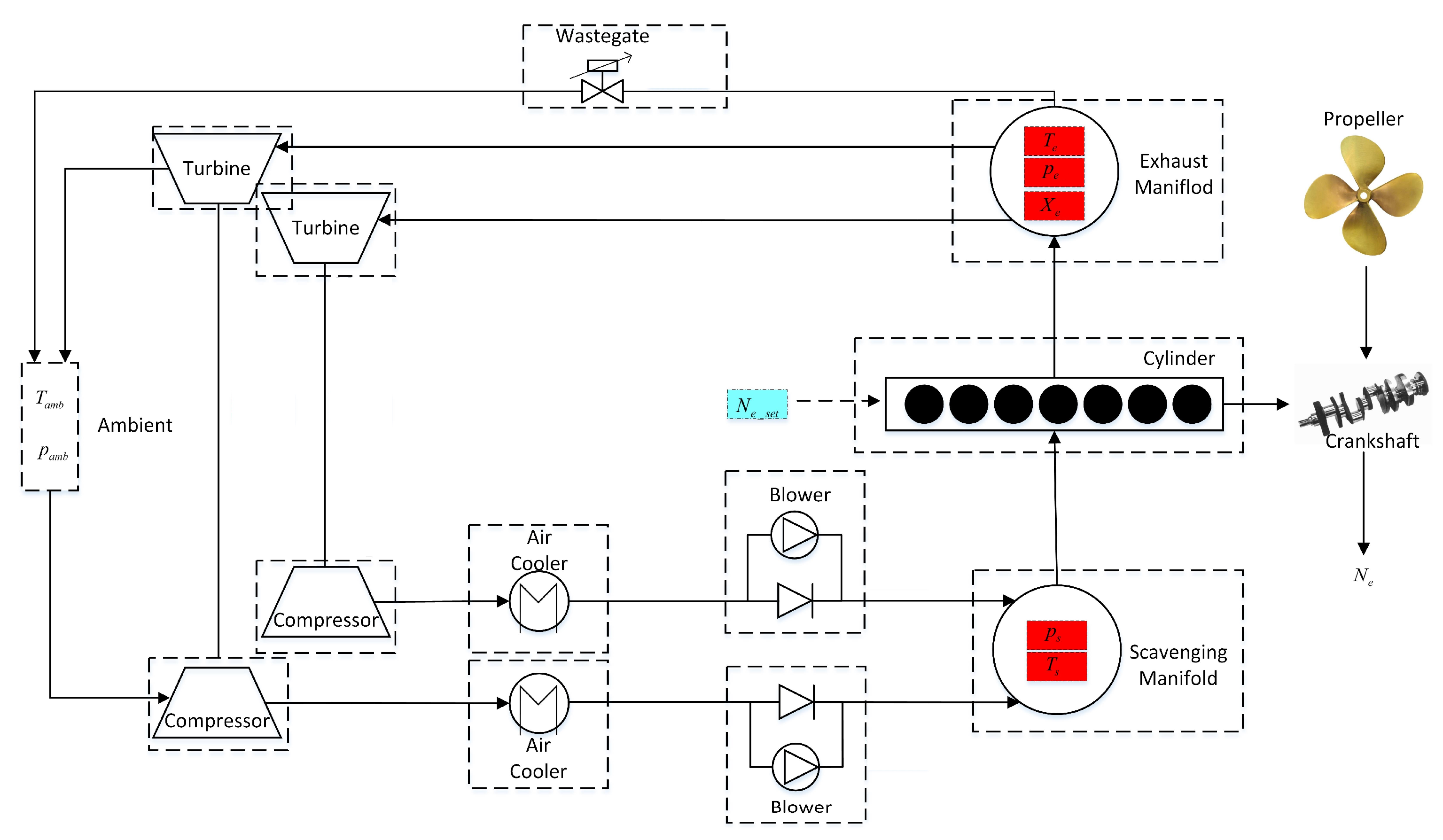
There are several model parameters in the cylinder pressure analytic model to be calibrated as following:
  • The compression and expansion polytropic index;
  • The pressure and temperature at the reference point of the compression polytropic process;
  • Wiebe function model parameters.

4.2.1. Calibration of Poyltropic Index

The polytropic process can be expressed as p V n = c o n s t and it can be transformed to ln p + n ln V = c o n s t by taking the logarithm of each side. Consequently, by setting ln V and ln p as the horizontal and vertical coordinate, respectively, a straight line can be obtained with the negative of its slope equal to the polytropic index [17]. 
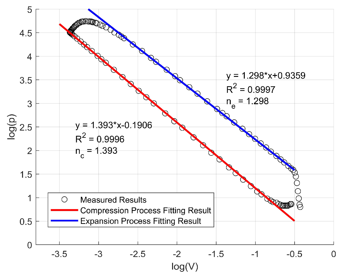
Figure 15 presents the estimation result of n c o m p and n exp for a certain operating condition. As can be observed from this figure, strong linear relationship exists between ln V and ln p with R2 larger than 0.999 for both the compression and expansion phase, which verifies the rationality of the assumption that the actual compression and expansion process can be approximately by the polytropic process.
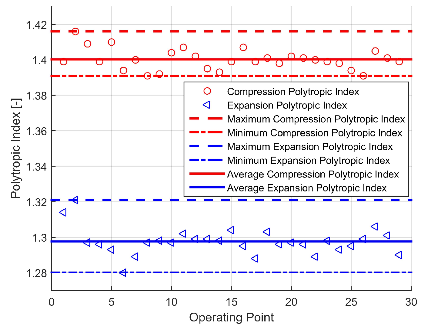
Figure 16 provides the compression and expansion polytropic index estimation results for 29 known engine operating points. These operating points are measured on-board a ship and cover a wide range of operating conditions, which are named as A1 to A29 in this paper. For n c o m p , its maximum and minimum value is 1.416 and 1.391, respectively, with a standard deviation of 0.0058; for n exp , its maximum and minimum value is 1.321 and 1.280, respectively, with a standard deviation of 0.0076. The results indicate that the polytropic index will not change significantly with the engine operating conditions. Actually, it was revealed by Brunt and Platts that the polytropic index was influenced by many factors including engine speed, working medium temperature, heat transfer, etc. [18]. However, due to lacking of experimental conditions especially for the marine large scale diesel engine investigated in this paper, it is difficult to derive correlations between the polytropic index and other engine performance parameters. Therefore, in this paper a 2-D look-up table is established to calculate the polytropic index with the engine speed and brake power as the input variables.

4.2.2. Calibration of p e v c and T e v c

In 
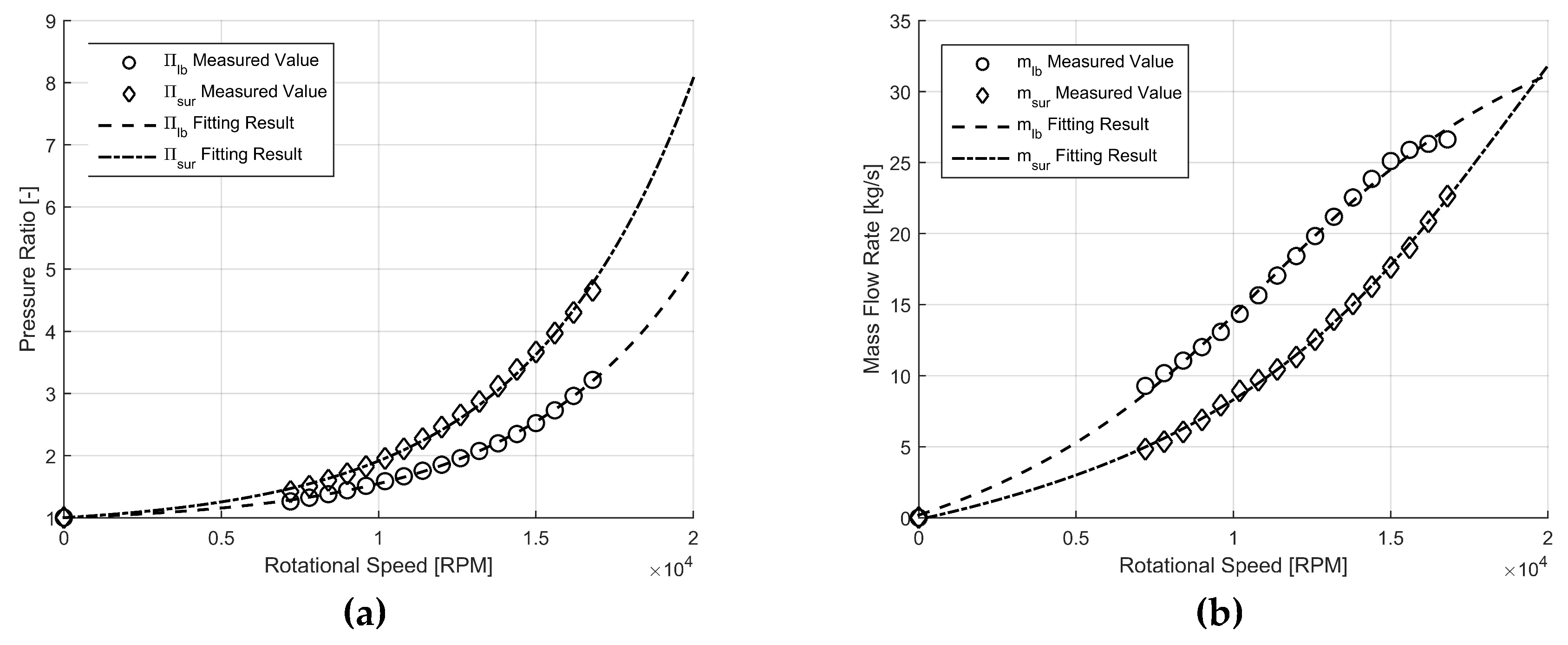
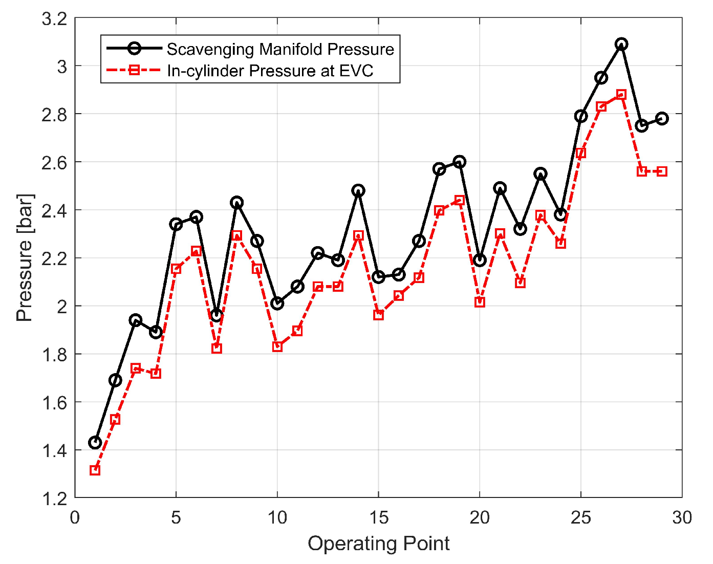
Figure 17, the measured value of p s and p e v c for the 29 known engine operating points are presented and compared. It can be observed from this figure that p s is always greater than p e v c 
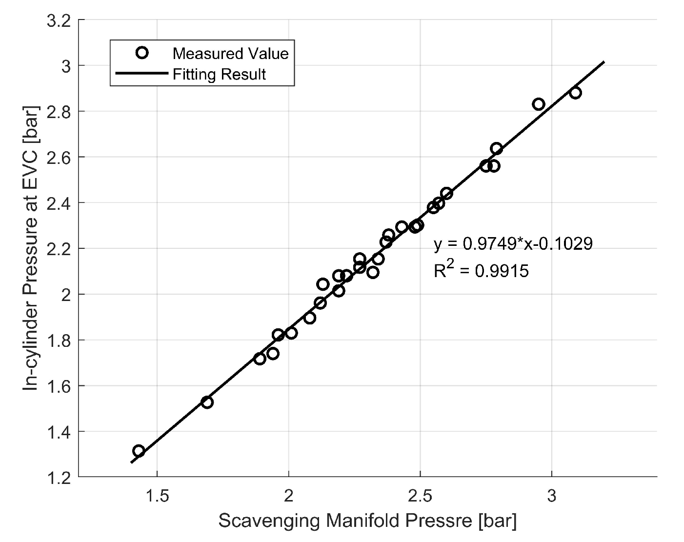
. In order to evaluate the quantitative relationship between p s and p e v c , they are set as the horizontal and vertical coordinate, respectively, as shown in Figure 18. It can be found from this figure that strong linear relationship exists between them with a R2 greater than 0.99. Consequently, p e v c can be expressed as a linear function of p s m , that is p e v c = 0.9749 p s 0.1029 in this paper.
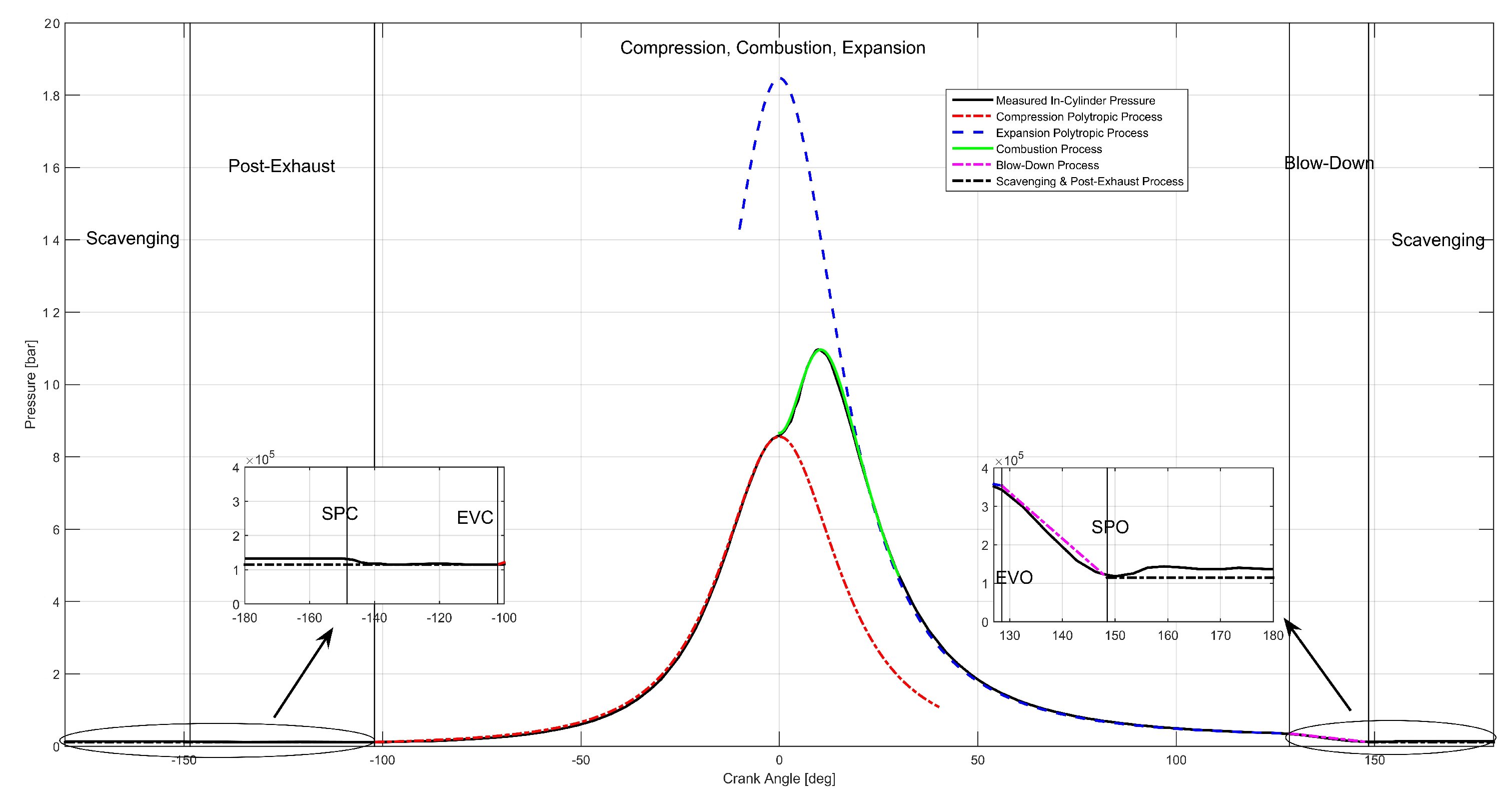
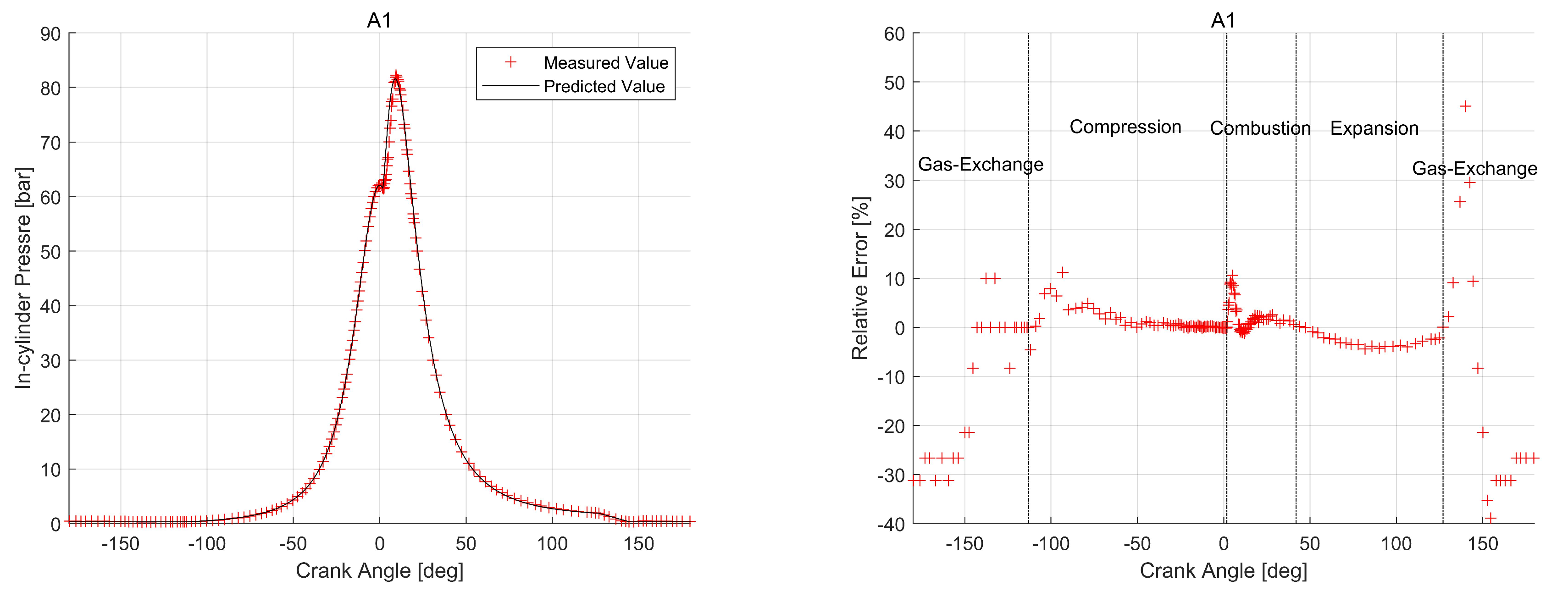
To guarantee the continuity of the simulated in-cylinder pressure trace during the scavenging and post-exhaust phase and also to reduce the model complexity, it is assumed that the in-cylinder pressure during the scavenging and post-exhaust phase is equal to p e v c . Although it can be observed from Figure 14 that this assumption will make the predicted in-cylinder pressure during the two phases slightly lower than the measured pressure, this will not significantly influence the model’s predictive accuracy because the pressure during the two phases is only about 0.5% of the in-cylinder maximum pressure. Based on this assumption, the slope and intercept of Equation (32) can be determined.
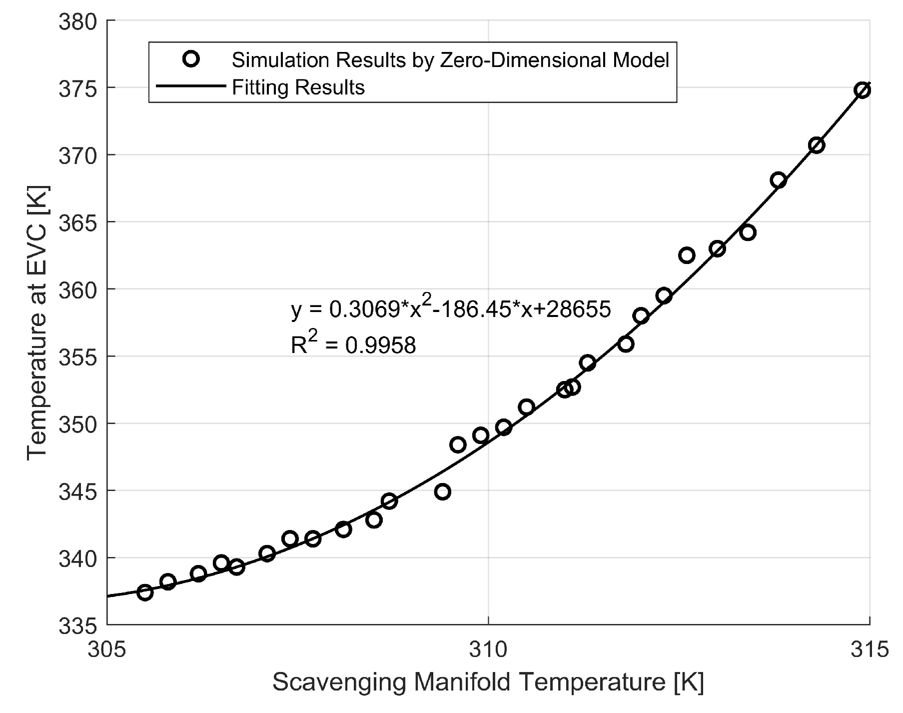
The research carried out by Tang et al [5] and Kharroubi and Söğüt [19] all indicated that relationship exists between the scavenging air temperature T s and T e v c . As T e v c is not measured both during the engine shop trial and on-board the ship, a 0-D engine model is adopted to investigate the relationship between T s and T e v c in this paper. In Figure 19, the simulated results of T s and T e v c are set as the horizontal and vertical coordinate. It can be found from this figure that a second-order polynomial is sufficient to capture the changing trend of T e v c with T s with a R2 of 0.9958, indicating satisfactory fitting results.

4.2.3. Calibration of Wiebe Function Model Parameters

In order to predict the in-cylinder pressure trace during the combustion phase, the Wiebe function is used to interpolate between the compression and expansion pressure. The general form of the single Wiebe function can be written as:
χ = 1 exp [ a ( θ θ s o c Δ θ C D ) m + 1 ]
where χ is the mass fraction burned (MFB); φ s o c is the start of combustion crank angle; Δ φ C D is the combustion duration; a is the efficiency factor; m is the form factor.
Step 1: Derive the MFB based on the measured in-cylinder pressure trace
Several classical MFB estimation methods can be found in the literature, such as the Apparent Heat Release model, the Gatowski model, the RW model, as well as the pressure ratio management (PRM) model [20]. In this paper, the PRM model is adopted to derive the MFB:
P R ( θ ) = p z ( θ ) p m ( θ ) 1
χ ( θ ) = P R ( θ ) P R max ( θ )
where PR is referred to as the pressure ratio; p z is the measured in-cylinder pressure; p m is the motored in-cylinder pressure; P R max is the maximum value of PR, which is used to normalize PR to obtain the MFB.
In this paper, the motored in-cylinder pressure p m is estimated by assuming the motored process as a polytropic process as it was done by many researchers [21,22,23]. In addition, it is assumed that the expansion polytropic index is equal to that of the compression process, the value of which can be estimated by following the calibration procedure as described in Section 4.2.1. Consequently, p m can be determined by using the following equation:
p m ( θ ) = p r e f ( V r e f V ( θ ) ) n m
where p r e f and V r e f are the pressure and volume at the reference point, which can be an arbitrary crank angle position between the EVC and SOC.
Step 2: Determine the number of single Wiebe function needed to be superposed
Ghojel pointed out that the form factor m in Wiebe function can reflect the distribution of combustion process, thus, the variation of m can be exploited to determine the number of single Wiebe function to be superposed [24]. Following this idea, the original single Wiebe function as shown in Equation (33) can be transformed to the following form by appropriate mathematical manipulation:
ln [ ln ( 1 χ ) / ln 0.5 ] = ( m + 1 ) ln ( θ θ s o c ) ( m + 1 ) ln ( θ 50 θ s o c )
where θ 50 is the crank angle corresponding to 50% MFB.
Set the ln ( θ θ s o c ) and ln [ ln ( 1 χ ) / ln 0.5 ] as the horizontal and vertical coordinate, respectively. If a straight line is obtained, a single Wiebe function is sufficient to simulate the combustion process accurately, otherwise, two or more single Wiebe functions are needed, the number of which can be estimated by the number of broken lines in the plane of ln ( θ θ s o c ) ~ ln [ ln ( 1 χ ) / ln 0.5 ] . For the 7S80ME-C9.2 marine engine, it is found that superposing two single Wiebe functions is sufficient in the whole engine operating envelope.
Step 3: Estimate the Wiebe function model parameters by using LSM
As mentioned in Step 2, double Wiebe function is sufficient to simulate the actual combustion process, which can be written as:
χ = ( 1 β ) { 1 exp [ a p ( θ θ s o c , p Δ θ C D , p ) m p + 1 ] } + β { 1 exp [ a d ( θ θ s o c , d Δ θ C D , d ) m d + 1 ] }
where subscript p and d represents premixed and diffusive combustion, respectively; β is the fraction of fuel burned during the diffusive combustion phase.
There are totally 9 model parameters in the double Wiebe function as shown in equation (38), making the model calibration process relatively laborious. Therefore, to reduce the number of Wiebe function model parameters to be calibrated, two assumptions are made herein:
(1) The premixed combustion duration is assumed to be equal to that of diffusive combustion. In addition, the crank angle range between 1% and 99% MFB is defined as the combustion duration by taking into account that the Signal to Noise Ratio (SNR) is relatively lower and the combustion is unstable at the start and end of the combustion;
(2) The crank angle at the start of premixed combustion is also assumed to be equal to that of diffusive combustion.
Based on the two assumptions, the number of Wiebe function model parameters to be calibrated reduces from 9 to 7; in addition, Δ θ C D and θ S O C can be estimated from the MFB curve beforehand. As a result, only 5 Wiebe function model parameters remain to be estimated.
Table 4 presents the calibration results of the Wiebe function model parameters for four operating points as well as the relevant predictive errors in MFB. As can be observed from this table, PE is less than 1.07 %, whereas MAE is less than 0.31 %, indicating the sufficient accuracy of double Wiebe function in simulating the actual combustion process in CI engines as well as the satisfactory calibration results.
To obtain an overall accurate Wiebe function, a 2-D look-up table is established for the Wiebe function model parameters with the engine speed and brake power as the inputs. In addition, it is found that the combustion duration can be well approximated by a linear function of the fuel injection rate.

4.3. Results

In this section, the in-cylinder pressure trace simulated by the analytic model under four different operating conditions are compared with the measured ones to validate its correctness as shown in Figure 20. It can be observed from this figure that the simulation results agree well with the measured results and can capture the variation trend of in-cylinder pressure trace with crank angle during each working phase. During the gas exchange phase (blow-down, scavenging and post-exhaust), the relative errors of the simulation results are relatively higher than the other phases, which is mainly caused by the simplifications and assumptions made for these phases, i.e., two simple linear functions are adopted to approximate the in-cylinder pressure trace; however, it should be noted that the absolute errors during the gas exchange phase are less than 0.15 bar, which is still satisfactory with respect to the variation range of in-cylinder pressure during the whole working cycle. During the combustion phase, the relative errors of most of the simulation results are less than 5%, which is mainly benefiting from the effective calibration of Wiebe function model parameters as introduced in Section 4.2.3. It should be noted that by superposing more single Wiebe functions, the simulation accuracy during the combustion phase will improve, but this will make the Wiebe function model parameters calibration process laborious. Actually, the current simulation accuracy is already satisfactory to some extent. At the start of compression phase, the relative errors of part of the simulation results approach 20%, which is maybe attributed to two reasons: (1) the absolute value of in-cylinder pressure is relatively lower and small absolute errors will lead to obvious relative errors; (2) the actual compression process is approximated by a polytropic process. Note that as part of the input variables of the analytic model are from the MVEM, thus the predictive errors of MVEM will transform to the analytic model and lead to predictive errors.
For practical engineering practice, the marine engineers normally judge the engine’s operation status by checking the compression pressure p c o m p , maximum pressure p max and its crank angle position θ p , max . Table 5 compares the predicted and measured results of p c o m p , p max and θ p , max . As can be observed from this table, the cylinder pressure analytic model is capable of predicting p c o m p and p max satisfactorily with relative errors less than 1%. Although the relative errors of θ p , max are relatively higher, the absolute errors are generally less than one crank angle, indicating that the predictive accuracy can be accepted to some extent.
The inputs of the analytic model, such as scavenging air pressure and temperature and engine speed, are completely from the MVEM and the calculation process does not influence the MVEM; however, it should be noted that the MVEM and the cylinder pressure analytic model have different simulation speed, which must be handled when they are coupled together and applied in the engine room simulator. Aiming at this problem, two threads are adopted to depart the analytic model from the MVEM as shown in Figure 21. At steady state conditions, the simulation results of the MVEM are the same in every engine cycle, meaning that the engine performance parameters transformed to the analytic model also remain unchanged, therefore, the in-cylinder pressure trace simulated by the analytic model will also be the same in every engine cycle; on the other hand, the in-cylinder pressure trace is not required to be updated in real-time in the engine room simulator, and the “Pressure-Crank Angle” diagram or the “Pressure-Volume” diagram need to be displayed only when the user switches to the corresponding simulation interfaces. Based on the two factors, at steady state conditions, the in-cylinder pressure trace only needs to be calculated for one engine cycle by the analytic model, therefore, the running speed of the whole model can be as fast as the MVEM.
During the transient process, the engine performance parameters and the in-cylinder pressure trace are different in every engine cycle; on the other hand, the MVEM and the cylinder pressure analytic model have different simulation speed. Therefore, in order to keep the simulation results in sync, the MVEM has to wait for some time before analytic model completes the calculation of an engine cycle as shown in Figure 21a, as a result, the simulation speed of the whole engine model is determined by the cylinder pressure analytic model, which is actually slower than the MVEM. To accelerate the simulation speed of the whole model, the idea of abandoning engine cycles is adopted. Figure 21b presents the case where the calculation frequency of the MVEM is two times the analytic model, meaning that the MVEM has already completed the calculation of two engine cycles when the analytic model only completes the calculation of one engine cycle. Figure 21c presents the case where the calculation frequency of the MVEM is many times the analytic model. By adopting this method, we can keep the MVEM and the cylinder pressure analytic model in sync, furthermore, the simulation speed of the whole model will get faster if more engine cycles are abandoned by the analytic model. The relationship between the number of abandoned cycles X and the reduced time Y can be expressed as Y=X/(X+1). It should be noted that the synchronization mentioned above is a fake synchronization during the transient process and this is because that the current simulated in-cylinder pressure trace simulated by the analytic model does not correspond to the current engine operating conditions outputted by the MVEM but falls behind to some extent.
To assess the improvement in simulation speed of the extended MVEM developed in this paper, it is compared with the merged model developed by Tang et al., where the 0-D model was adopted to calculate the in-cylinder pressure and the MVEM was used to simulate other engine performance parameters with the similar synchronization approach as shown in Figure 21 [5]. The comparison of actual execution time for a 100 s simulation time is presented in Table 6.
As can be found from Table 6, the engine model developed in this paper is able to achieve similar actual execution time of about one second but only four cycles are abandoned, whereas it is 49 for the merged model developed by Tang et al. [5]. This is due to the fact that the cylinder pressure analytic model runs much faster than the 0-D model and therefore similar actual execution time can be obtained by abandoning less number of engine cycles. As a result, the model developed in this paper can capture the transient response of the in-cylinder pressure trace more accurately.

5. Conclusions

In this article, a marine two stroke diesel engine MVEM with in-cylinder pressure trace predictive capability and a novel compressor model was developed.
A previous study carried out by the first author indicated that none of the compressor empirical mass flow rate models existing in the literature appears to achieve satisfactory predictive accuracy in the whole operating area. To solve this problem, the compressor whole operating area was divided into design, LS, HS and LPR operating areas by defining zonal division standard with appropriate functions, and then the compressor mass flow rate model that achieved the best predictive accuracy was selected for each operating area. In addition, an appropriate blending function was applied when the operating point enters into the LRP area from other areas to avoid the possible discontinuity.
The zonal compressor isentropic efficiency model proposed in this paper was based on the Hadef model. By dividing the whole “Mass flow rate—actual specific enthalpy change” plane into several zones by using the iso-speed curves available in the performance map, the working characteristics of compressor within different speed range can be captured much more accurately. It was revealed from the simulation results that with respect to the original Hadef model, the predictive accuracy of the zonal isentropic efficiency model was effectively improved. In addition, satisfactory extrapolation accuracy was obtained with this zonal compressor isentropic efficiency model.
As can be found from the trajectory of the compressor operating points during the transient process, the compressor model proposed in this paper is able to extrapolate to the LS and HS off-design operating areas reasonably and robustly; in addition, by comparing with the measured data provided in the engine shop trial report, the predictive accuracy of the engine performance parameters relevant to the turbocharger were all satisfactory at each steady state loading condition. Based on these simulation results, the fidelity of the proposed compressor model was validated. Due to the significant influence of the compressor on the engine steady state performance and transient response, the compressor model proposed in this paper is very helpful for improving the MVEM’s predictive accuracy in the whole engine operating envelope.
By adapting the cylinder pressure analytic model to the 7S80ME-C9.2 marine two-stroke diesel engine, the MVEM is able to predict the in-cylinder pressure trace without impairing its merit in running speed. For achieving satisfactory predictive accuracy, the model parameters of the analytic model were finely calibrated by using the measured data and a 0-D engine model. At steady state condition, the extended MVEM runs as fast as the MVEM. During the transient process, the extended MVEM is able to achieve the running speed as similar as the MG model (0D + MVEM) proposed by Tang et al. [5] but captures the transient response of the in-cylinder pressure trace more accurately.
Although some sub-models of the MVEM are needed to be re-calibrated if another engine is to be modeled, they can be calibrated readily by only using the engine shop trial report and relevant performance maps. As a result of the lack of sufficient engine measured data, 2-D look-up tables were developed to calculate Wiebe function model parameters as well as the compression and expansion polytropic index. Although rapid calculation speed and satisfactory interpolation accuracy can be achieved with the 2-D look-up table, its extrapolative ability is big issue. In the future study, more measured engine data will be gathered to develop correlations between the model parameters and the engine performance parameters to enhance their extrapolative ability.

Author Contributions

H.S. contributed to the development of mathematical models, analysis of simulation results and the writing of the manuscript. J.Z. provided research conditions, team support and financial support. B.Y. and B.J. gave some useful suggestions. All authors have read and agreed to the published version of the manuscript.

Funding

This work was supported by the National Natural Science Foundation of China, grant number 51479017, and the Fundamental Research Funds for the Central Universities, grant number 3132019315.

Acknowledgments

The authors are especially grateful to Tang, who provided important technical support.

Conflicts of Interest

The authors declare no conflict of interest.

Nomenclature

a Wiebe function efficiency factor (−)/model parameter (−) n polytropic index (−)/number (−)
b model parameter (−) N rotational speed (RPM)
A area (m2) p pressure (pa)
C flow coefficient (−) P power (W)
c p constant pressure specific heat (J/kg K) p ¯ mean effective pressure (pa)
c v constant volume specific heat (J/kg K) Q torque (N m)
h specific heat (J/kg) Q ˙ h t heat transfer rate (W)
H L H V fuel lower heating value (J/kg) R gas constant (J/kg K)
J moment of inertia (kg m2) T temperature (K)
K p propeller torque coefficient (−) V d cylinder displacement volume (m3)
k model parameter (−) V ˙ volume flow rate (m3/s)
m ˙ mass flow rate (kg/s) V cylinder instantaneous volume (m3)
m Wiebe function form factor (−)/mass (kg)
Greek symbols
γ specific heat ratio (−) Γ expansion ratio (−)
θ crank angle (deg) ω angular velocity (rad/s)
ζ fuel chemical energy proportion in the exhaust gas (−) ϕ fuel air equivalent ratio (−)
η efficiency (−) χ mass fraction burned (−)
Π pressure ratio (−)
Subscripts
aairiindicated
acair coolerininlet
afair filterisisentropic
ambambient lblower bound
actactualmmotored
bbrakeoutoutlet
blblowerppropeller/premixed
ccompressorpepost exhaust
cwcooling waterrefreference
compcompressionsscavenging manifold
combcombustionsursurging
CDcombustion durationshshaft
ddiffusive scavscavenging
eexhaust manifold/engine/exhaust gassocstart of combustion
ellellipsetturbine
expexpansiontcturbocharger
exhexhaustzcylinder
ffuel/fricative

References

  1. Theotokatos, G.; Guan, C.; Chen, H.; Lazakis, I. Development of an extended mean value engine model for predicting the marine two-stroke engine operation at varying settings. Energy 2018, 143, 533–545. [Google Scholar] [CrossRef] [Green Version]
  2. Mavrelos, C.; Theotokatos, G. Numerical investigation of a premixed combustion large marine two-stroke dual fuel engine for optimising engine settings via parametric runs. Energy Convers. Manag. 2018, 160, 48–59. [Google Scholar] [CrossRef] [Green Version]
  3. Stoumpos, S.; Theotokatos, G.; Boulougouris, E.; Vassalos, D.; Lazakis, I.; Livanos, G. Marine dual fuel engine modelling and parametric investigation of engine settings effect on performance-emissions trade-offs. Ocean Eng. 2018, 157, 376–386. [Google Scholar] [CrossRef] [Green Version]
  4. Eriksson, L.; Nielsen, L. Modeling and Control of Engines and Drivelines; John Wiley and Sons Ltd.: Hoboken, NJ, USA, 2014. [Google Scholar]
  5. Tang, Y.Y.; Zhang, J.D.; Gan, H.B.; Jia, B.Z.; Xia, Y. Development of a real-time two-stroke diesel engine model with in-cylinder pressure prediction capability. Appl. Energy 2017, 194, 55–70. [Google Scholar] [CrossRef]
  6. Altosole, M.; Campora, U.; Figari, M.; Laviola, M.; Martelli, M. A diesel engine modelling approach for ship propulsion real-time simulators. J. Mar. Sci. Eng. 2019, 7, 138. [Google Scholar] [CrossRef] [Green Version]
  7. Nikzadfar, K.; Shamekhi, A.H. An extended mean value model (EMVM) for control-oriented modeling of diesel engines transient performance and emissions. Fuel 2015, 154, 275–292. [Google Scholar] [CrossRef]
  8. Theotokatos, G. On the cycle mean value modelling of a large two-stroke marine diesel engine. Proc. Inst. Mech. Eng. Part M J. Eng. Marit. Environ. 2010, 224, 193–205. [Google Scholar] [CrossRef]
  9. Baldi, F.; Theotokatos, G.; Andersson, K. Development of a combined mean value-zero dimensional model and application for a large marine four-stroke diesel engine simulation. Appl. Energy 2015, 154, 402–415. [Google Scholar] [CrossRef] [Green Version]
  10. Eriksson, L.; Andersson, I. An analytic model for cylinder pressure in a four stroke SI engine. In Proceedings of the SAE 2002 World Congress, Detroit, MI, USA, 4–7 March 2002. [Google Scholar]
  11. Shen, H.S.; Zhang, J.D.; Yang, B.C.; Jia, B.Z. Development of an educational virtual reality training system for marine engineers. Comput. Appl. Eng. Educ. 2019, 27, 580–602. [Google Scholar] [CrossRef]
  12. Theotokatos, G.; Tzelepis, V. A computational study on the performance and emission parameters mapping of a ship propulsion system. J. Eng. Marit. Environ. 2015, 229, 58–76. [Google Scholar] [CrossRef] [Green Version]
  13. Tu, H. Investigation on the Performance Optimization Method for Large Containership Propulsion Engine at Slow Steaming Conditions. Ph.D. Thesis, Wuhan University of Technology, Wuhan, China, 2015. [Google Scholar]
  14. Llamas, X.; Eriksson, L. Parameterizing compact and extensible compressor models using orthogonal distance minimization. J. Eng. Gas Turbines Power 2017, 139, 012601. [Google Scholar] [CrossRef]
  15. Shen, H.S.; Zhang, C.; Zhang, J.D.; Yang, B.C.; Jia, B.Z. Applicable and comparative research of compressor mass flow rate and isentropic efficiency empirical models to marine large-scale compressor. Energies 2020, 13, 47. [Google Scholar] [CrossRef] [Green Version]
  16. Hadef, J.E.; Colin, G.; Chamaillard, Y.; Talon, V. Physical-based algorithms for interpolation and extrapolation of turbocharger data maps. SAE Int. J. Engines 2012, 5, 363–378. [Google Scholar] [CrossRef]
  17. Baratta, M.; Misul, D. Development and assessment of a new methodology for end of combustion detection and its application to cycle resolved heat release analysis in IC engines. Appl. Energy 2012, 98, 174–189. [Google Scholar] [CrossRef]
  18. Brunt, M.F.; Platts, K.C. Calculation of heat release in direct injection diesel engines. In Proceedings of the SAE 1999 International Congress and Exposition, Detroit, MI, USA, 1–4 March 1999. [Google Scholar]
  19. Kharroubi, K.; Söğüt, O.S. Modelling of the propulsion plant of a large container ship by the partition of the cycle the main diesel engine. J. Eng. Marit. Environ. 2019. [Google Scholar] [CrossRef]
  20. Eriksson, L.; Thomasson, A. Cylinder state estimation from measured cylinder pressure traces—A survey. IFAC PapersOnLine 2017, 50, 11029–11039. [Google Scholar] [CrossRef]
  21. Oh, S.; Min, K.; Sunwoo, M. Real-time start of a combustion detection algorithm using initial heat release for direct injection diesel engines. Appl. Therm. Eng. 2015, 89, 332–345. [Google Scholar] [CrossRef]
  22. Choe, D.; Lee, M.; Lee, K.; Sunwoo, M.; Jin, K.K.; Chang, K.; Shin, K. SOC detection of controlled auto-ignition engine. In Proceedings of the 14th Asia Pacific Automotive Engineering Conference, Hollywood, CA, USA, 5–8 August 2007. [Google Scholar]
  23. Zhu, G.; Daniels, C.F.; Winkelman, J. MBT timing detection and its closed-loop control using in-cylinder pressure signal. In Proceedings of the 2003 Powertrain and Fluid Systems Conference and Exhibition, Pittsburgh, PA, USA, 27–30 October 2003. [Google Scholar]
  24. Ghojel, J.I. Review of the development and applications of the Wiebe function: A tribute to the contribution of Ivan Wiebe to engine research. Int. J. Engine Res. 2010, 11, 297–312. [Google Scholar] [CrossRef]
Figure 1. Mean value engine model (MVEM) structure.
Jmse 08 00204 g001
Figure 2. Compressor performance map.
Jmse 08 00204 g002
Figure 3. Zone division standard of the compressor performance map.
Jmse 08 00204 g003
Figure 4. Measured pressure ratio and mass flow rate at the boundary of surging zone and low pressure ratio zone and corresponding fitting result: (a) pressure ratio; (b) mass flow rate.
Jmse 08 00204 g004
Figure 5. Prediction and extrapolation result of the zonal compressor mass flow rate model.
Jmse 08 00204 g005
Figure 6. Relationship between actual specific enthalpy change and mass flow rate at each rotational speed condition (interval between each iso-speed curve is 600 RPM).
Jmse 08 00204 g006
Figure 7. Predictive result and error distribution for Hadef isentropic efficiency model: (a) predictive result; (b) error distribution.
Jmse 08 00204 g007
Figure 8. Prediction result and error distribution for compressor zonal isentropic efficiency model: (a) predictive result; (b) error distribution.
Jmse 08 00204 g008
Figure 9. Prediction and extrapolation result of the zonal compressor isentropic efficiency model.
Jmse 08 00204 g009
Figure 10. Extrapolation result of the zonal compressor isentropic efficiency model: (a) LS (Low Speed) area extrapolation result; (b) HS (High Speed) area extrapolation result.
Jmse 08 00204 g010
Figure 11. Steady state simulation results and comparison with engine shop trial report and CEAS (Computerized Engine Application System): (a) brake power; (b) brake specific fuel consumption (BSFC); (c) exhaust manifold pressure; (d) exhaust manifold temperature; (e) scavenging manifold pressure; (f) scavenging manifold temperature; (g) compressor outlet temperature; (h) turbine outlet temperature; (i) turbocharger rotational speed; (j) fuel-air equivalence ratio.
Jmse 08 00204 g011aJmse 08 00204 g011b
Figure 12. Simulation results for the engine transient operation with setting speed changes: (a) engine rotational speed; (b) turbocharger rotational speed; (c) exhaust manifold and turbine outlet temperature; (d) scavenging manifold and compressor outlet temperature; (e) scavenging and exhaust manifold pressure; (f) fuel-air equivalence ratio; (g) brake power; (h) fuel index; (i) BSFC; (j) compressor operating points trajectory.
Jmse 08 00204 g012
Figure 13. Simulation results for the engine transient operation with resistant torque changes: (a) engine rotational speed; (b) turbocharger rotational speed; (c) exhaust manifold and turbine outlet temperature; (d) scavenging manifold and compressor outlet temperature; (e) scavenging and exhaust manifold pressure; (f) fuel-air equivalence ratio; (g) brake power; (h) fuel index; (i) BSFC; (j) compressor operating points trajectory.
Jmse 08 00204 g013
Figure 14. Basic idea of the cylinder pressure analytic model (SPC: Scavenging ports closing; SPO: Scavenging ports opening; EVC: Exhaust valve closing; EVO: Exhaust valve opening).
Jmse 08 00204 g014
Figure 15. Relationship between log(V) and log(p) and linear fitting result for the compression and expansion process.
Jmse 08 00204 g015
Figure 16. Compression and expansion polytropic index results for the 29 known operating conditions.
Jmse 08 00204 g016
Figure 17. Comparison between scavenging manifold pressure and in-cylinder pressure at exhaust valve closing (EVC) based on measured data.
Jmse 08 00204 g017
Figure 18. Fitting result between scavenging manifold pressure and in-cylinder pressure at EVC based on measured data.
Jmse 08 00204 g018
Figure 19. Fitting result between scavenging manifold temperature and in-cylinder temperature at EVC based on the 0-D model.
Jmse 08 00204 g019
Figure 20. Prediction result and error distribution of the cylinder pressure analytic model: (a) predictive results; (b) error distribution.
Jmse 08 00204 g020aJmse 08 00204 g020b
Figure 21. Synchronization approach for the MVEM and the cylinder pressure analytic model: (a) X = 0; (b) X = 1; (c) the calculation frequency of the MVEM is many times the analytic model.
Jmse 08 00204 g021
Table 1. Main Technical parameters of 7S80ME-C9.2 diesel engine at MCR (Maximum Continuous Rating).
ParametersValue
Number of cylinder (−)7
Cylinder bore (mm)800
Stroke (mm)3450
Speed (rpm)72
Power (kW)25190
Maximum pressure (MPa)17.1
Mean brake effective pressure (bar)17.3
Firing order1-7-2-5-4-3-6
Specific fuel oil consumption (g/kW⋅h)165.9
Table 2. Error evaluation criteria result for Hadef model and zonal compressor isentropic efficiency model.
Model R c 2 R D max ( % ) M A P E ( % ) P E B ± 5 % ( % ) P E B ± 10 % ( % )
Hadef model0.96756.79670.903898.9619100
Zonal isentropic efficiency model0.98582.55350.6428100100
Table 3. Relative error of the engine performance parameters.
Engine Load (%)1525507580100
Error (%)
Brake Power0.74−0.940.630.550.350.04
Brake Power [5]null1.612.210.380.460.56
BSFC−0.180.58−0.47−0.50−0.06−0.74
BSFC [5]null3.021.700.380.460.56
Scavenging manifold pressure1.431.803.451.942.141.16
Scavenging manifold pressure [5]null−3.23−1.2700.280
Exhaust manifold pressure−3.20−5.21−3.19−2.63−1.26−0.89
Exhaust manifold temperature−0.02−1.70−2.38−2.27−1.92−1.87
Exhaust manifold temperature [5]null0.731.751.31−1−0.22
Turbocharger speed −0.043−0.551.690.140.740.49
Turbocharger speed [5]null−2.43−0.98−1.14−2.08−1.34
Compressor outlet temperature1.21−0.422.680.230.60−0.22
Turbine outlet temperature3.592.853.422.312.233.09
Table 4. Wiebe parameters and predictive error.
Operating PointA2A8A14A25
a p 3.4153.7693.453.319
a d 23.823.7217.2812.71
m p 1.1481.2921.5782.2
m d 1.0060.97290.90350.7247
β 0.67490.64810.69920.8023
P E (%) 11.070.810.950.78
M A E (%) 20.310.270.190.25
1PE: Peak Error; 2MAE: Mean Absolute Error.
Table 5. Prediction error of the cylinder pressure analytic model.
p c o m p (bar) p max (bar) θ p max (deg)
A1PD162.181.69.0
MD262.282.39.5
RD(%) 3−0.16−0.85−5.26
A3PD73.9102.29.0
MD73.8102.78.6
RD (%)0.14−0.494.65
A14PD89.5114.511.1
MD89.7114.110.3
RD (%)−0.220.357.77
A25PD100.3125.810.8
MD101.3126.29.7
RD (%)−0.99−0.3211.34
1 Predicted value; 2 Measured value; 3 Relative error.
Table 6. Comparison of simulation speed.
ModelAbandoned CyclesExecution Time (s)Simulation Time (s)
Tang et al. [5]491.002100
This paper40.946100

