Thermal Infrared Spectral Characteristics of Bunker Fuel Oil to Determine Oil-Film Thickness and API

Abstract

Remote sensing is an important method for monitoring marine oil-spill accidents. However, methods for measuring oil-film thickness remain insufficient. Due to the stable differences in the surface emissivity and temperature of oil and water, the oil film can be detected using thermal infrared. This study measured emissivity of seven different oil-film thicknesses and seven different American Petroleum Institute (API) densities, and analyzed the spectral characteristics. Results show an optimal wavelength position for oil-film thickness and fuel API density monitoring is 12.55 μm. Principal component analysis and continuum removal methods were used for data processing. Stepwise multiple linear regression was used to establish relationships between emissivity and oil slick thicknesses and API densities. Oil-film thickness and fuel API density data were analyzed by principal component analysis and continuum removal before regression analysis. The spectral emissivity data was convolved into Advanced Spaceborne Thermal Emission and Reflection Radiometer (ASTER) and Advanced Very High Resolution Radiometer (AVHRR) thermal bands to determine potential of the sensor in oil-film detection. The result shows that neither could be used to estimate thickness. The AVHRR-4 band and band 12 and 13 of the ASTER could be used to separate oils from water and have potential to distinguish different oil types.

1. Introduction

With the development of oil extraction and maritime transportation, marine oil-spill accidents frequently occur, causing severe damage to the marine environment [1,2]. In addition, oil spills contain aromatic hydrocarbons, which are highly toxic to humans [3]. Oil can also be adsorbed on the coastline and damages the local ecological environment [4]. Obtaining information on oil spills is essential for timely action to reduce environmental and ecological pollution. Remote sensing is a detection technology that can provide macro and dynamic observations and is not limited by geographical location and human factors, and is one of the most effective means to monitor the diffusion range and oil thickness following an oil spill [5,6,7]. Commonly used oil-spill monitoring technologies include the synthetic aperture radar [8], optical remote sensing [9], and laser fluorescence [10]. The synthetic aperture radar is widely used in oil-spill detection because of its all-day and all-weather capabilities [11]. However, synthetic aperture radar satellite measurements are affected by weather conditions and oil thickness [12]. With the development of charge-coupled device (CCD) cameras, optical remote sensing gained both higher resolution and lower cost. However, CCDs can be interfered with by other background information such as reflected sunlight [13]. Laser fluorescence is a form of active remote sensing with all-weather characteristics, and fuel oil can show strong fluorescence characteristics to distinguish it from other substances [14]. However, laser fluorescence has obvious deficiencies in measuring fuel thickness [12]. Thermal infrared analysis distinguishes oil on the sea surface by thermal comparison. Because the emissivity of water and oil are different, thermal contrast is generated, and the emissivity depends on the thickness of the oil slick [15]. During the daytime, thick oil slicks become warmer than the surrounding water while thinner, detectable slicks appear cooler. This reverses at nighttime [16,17]. A thin film interference theory-based model is used to describe the thickness-dependent contrast between the background water and the sea surface covered by crude oil [18,19]. The thermal infrared emissivity of fuels was measured and analyzed using statistical methods [20,21,22]. At the same time, the different emission spectra of the fuels were detected, and a relationship between the fuel emissivity and the American Petroleum Institute (API) density was obtained.

At present, thermal infrared technology is widely used in vegetation and soil detection. Among these [23], the relationship between the emissivity spectrum of the thermal infrared region and the leaf area index is obtained. The thermal infrared region is used to study soil moisture [24], and it has been proven that the long-wave infrared band is more accurate than visible-near infrared and shortwave infrared for the prediction of soil properties [25]. Some studies have applied thermal infrared technology to fuel-oil measurements, using regression analyses, to test the degree of soil oil pollution [26], and through experiments have identified midday as the optimal detection time for oil slicks [27]. The relationship between the wavelength and emissivity of the oil-film thickness in the range of 0–380 μm was obtained by using the thermal infrared band to detect the oil slick thickness [22]. It was concluded that the thermal infrared emissivity of oil films changes greatly when they are thin and that the emissivity changes slightly with thickness as the oil-film thickness increases. It was also concluded that the correlation between emissivity and thickness changes greatly in the range of 11.7–13 μm, and that the correlation is weak. The emissivity changes considerably with an increase in the oil-film thickness at 11.7 μm and 12.55 μm, and so can be used to detect the oil-film spectral response [22]. However, the multicollinearity of the spectrum for statistical analysis was not considered. In this study, the aforementioned thermal infrared fuel detection methods were integrated. The thickness of an oil slick was measured in the thermal infrared band, and the data emissivity was statistically analyzed.

The purpose of this study is to determine the thickness of an oil film by detecting its thermal infrared emissivity. Considering the multicollinearity of spectral emissivity data, a model was built using stepwise multiple linear regression. Principal component analysis and continuum removal were used to reduce the data dimensions. This study also used different fuel types for analysis to determine the relationship between different oil emissivity and its API density. Different thermal infrared sensors were also used to resample the spectral data to determine the potential of these sensors for measuring oil films and identifying fuel types.

2. Materials and Methods

2.1. Experimental Conditions

The experiment was conducted from 15 to 16 August 2019. There were no moving, tall objects in the vicinity of the experimental site. The measurement time is recommended in the early morning or late afternoon. At this time, the sample temperature is relatively stable. It can avoid the change of targets’ temperature caused by atmospheric convection, and avoid the unstable downward radiation of atmosphere. Also, the temperature of the instrument could remain stable. The mean air temperature during the experiment was 30 °C. During the measurement, the sky was cloud free and there was no wind, which may reduce the influence of the atmosphere.

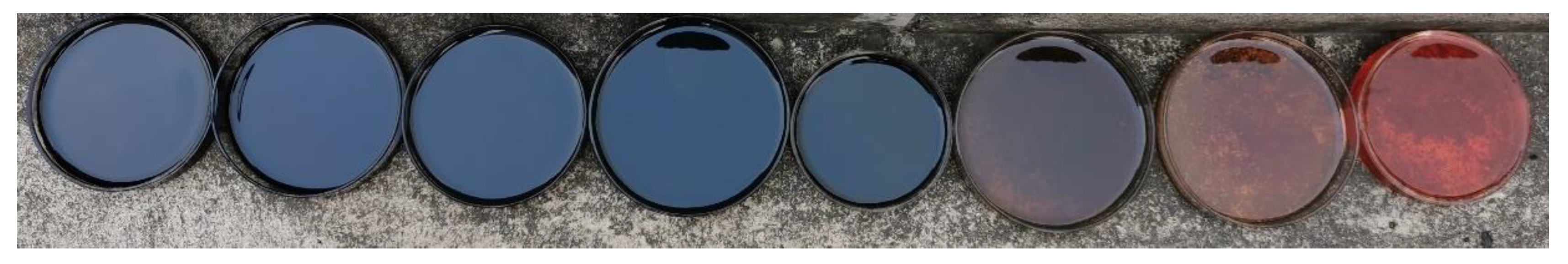
2.2. Oil Sample and Its Measurement

The experiment consisted of two parts. Firstly, water from Bohai Bay was placed into a beaker, and the fuel (numbered 0) was gradually added onto the water surface. In the oil-film experiment, the fuel used was Great Wall Marine Lubricant with a viscosity (100 °C) of 19.9 mm² / s. A Teflon beaker was used because the Teflon material is not hydrophilic and has no wall hanging phenomenon. The diameter of the beaker was 190 mm. The beaker was placed directly below the spectrometer, the height of the tripod adjusted, and the water surface was 1 meter away from the spectrometer lens. Oil was applied to the center of the water surface with a syringe. The measurement was performed after about 5 min of adding oil, during which the oil could fully spread and reach the same temperature as the water. After the fuel had fully spread, a thermal infrared spectrometer was used to obtain the oil-film thermal infrared spectrum. The distribution of oil on the water surface is not uniform and the shape of an oil film is always irregular. This makes it difficult to calculate the area of oil film directely. Photos of the oil films were taken and geometric correction performed with ArcGIS (v. 10.0, ESRI). By using the shape-area calculation fuction in ArcGIS, we could obtain the area of oil films on the water surface. In the second part of the experiment, the experimental samples were fuels obtained from seven ships. The fuel was placed in a petri dish under the spectrometer to measure emissivity. The fuels of the seven ships were numbered from No. 1 to No. 7 and the API density of the seven oils is shown in

Table 1. Different American Petroleum Institute (API) density tables for different ship fuels used in this study.

Sample No.	No.1	No.2	No.3	No.4	No.5	No.6	No.7
API	25.04	27.04	28.13	34.99	34.97	33.38	29.30

. The fuel used in the experiment is shown in Figure 1.

2.3. Emissivity Calculation Principle

Under clear sky conditions, the thermal infrared radiation at the top of the atmosphere includes surface thermal infrared emission radiation, thermal path radiation, scattered solar radiation, direct solar radiation and scattered radiation reflected from the surface, and atmospheric thermal infrared radiation [28]. For the thermal infrared atmospheric window of 8–14 μm, the contribution of solar radiation was negligible, so the scattered solar radiation, the direct solar radiation reflected from the ground, and the scattered radiation could be ignored in the radiation transmission equation. The atmospheric radiation transmission equation in the thermal infrared band can be expressed as:

$$L\left(\lambda \right)=B\left(T_s,\lambda \right)\epsilon \left(\lambda \right)t\left(\lambda \right)+\left[1-\epsilon \left(\lambda \right)\right]L_{\downarrow }\left(\lambda \right)t\left(\lambda \right)+L_{\uparrow }\left(\lambda \right)$$

(1)

where λ is the wavelength; L(λ) is the radiation brightness received by the sensor; T_s is the physical temperature; B(T_s,λ) is the black body radiation brightness corresponding to the temperature T_s; ε(λ) is the emissivity at the wavelength λ; t(λ) is the atmospheric transmittance; L_↓ (λ) is the atmospheric downward radiation; and L_↑ (λ) is the upward radiance of the atmosphere. Because ground measurements were obtained and the objects were close to the sensor, it can be assumed that L_↑ (λ) was 0 and t(λ) is 1. The radiative transfer equation can be transformed into:

$$L\left(\lambda \right)=B\left(T_s,\lambda \right)\epsilon \left(\lambda \right)+\left[1-\epsilon \left(\lambda \right)\right]L_{\downarrow }\left(\lambda \right)$$

(2)

Here, L(λ) was provided by a 102F portable Fourier transform thermal infrared (FTIR) spectrometer, which can obtain the infrared thermal spectrum of ground objects with high spectral resolution. A temperature emissivity separation algorithm can calculate surface temperature and emissivity. The unknown quantities in the radiative transfer equation are the surface temperature T_s, the emissivity ε(λ), and the downward radiance L_↓ (λ) of the atmosphere. The downward radiance of the atmosphere is generally measured by a highly reflective gold plate:

$$L_{\downarrow }\left(\lambda \right)=\frac{L_{\mathrm{panel}}-{\epsilon }_{\mathrm{panel}}B\left(T_{\mathrm{panel}}\right)}{1-{\epsilon }_{\mathrm{panel}}}$$

(3)

where L_panel is the radiance reflected by the diffuse reflection plate received by the instrument; ε_panel is the emissivity of the diffuse reflection plate; and B(T_panel) is the black body radiation brightness corresponding to the diffuse reflection plate. The size was 10 × 10 cm, the surface was gold-plated, and the reflectivity was 0.6. Therefore, the object emissivity formula is:

$$\epsilon \lambda =\frac{L\left(\lambda \right)-\frac{L_{\mathrm{panel}}-{\epsilon }_{\mathrm{panel}}B\left(T_{\mathrm{panel}}\right)}{1-{\epsilon }_{\mathrm{panel}}}}{B\left(T_s,\lambda \right)-\frac{L_{\mathrm{panel}}-{\epsilon }_{\mathrm{panel}}B\left(T_{\mathrm{panel}}\right)}{1-{\epsilon }_{\mathrm{panel}}}}$$

(4)

2.4. Instrumentation and Spectral Measurements

The thermal infrared spectrum was measured and recorded by a 102F portable FTIR spectrometer. The observation range of the spectrometer was between 2–25 μm and the spectral resolution was 2 cm⁻¹. In this experiment, the emissivity range was 8–13 μm.

The FTIR spectrometer was fixed on a tripod that was positioned at a height of one meter from the ground. Liquid nitrogen was added to the spectrometer for cooling prior to the spectrometer being turned on. Calibration was performed using a black body [29]. In this experiment, the high temperature was set to 40 °C and the low temperature was set to 20 °C. After the calibration was completed, the blackbody was removed, the lens was rotated, and the gold plate was placed directly below the spectrometer lens so that the center of the gold plate covered the entire lens. The downward radiation of the atmosphere and the temperature of the gold plate were measured by a thermocouple thermometer. The fixed position of personnel was maintained during the experiment to reduce atmospheric radiation errors. The gold plate was removed, the oil film was fixed under the lens, and the surface emissivity of the oil film that formed on the water surface of the petri dish (after the oil-film diffusion was static) was measured.

2.5. Statistical Analysis

Spectral emissivity data showed strong collinearity between wavelengths, which rendered the data redundant. The data required processing to eliminate the multicollinearity of the data. This study principally used the following methods to analyze the measurement data: (1) principal component analysis; (2) continuum removal; and (3) stepwise multiple linear regression. Principal component analysis and continuum removal were used to eliminate the multicollinearity and highlight the significant characteristics of spectral data. The 1st and 2nd principal components were selected to perform stepwise multiple linear regression, in which the components were input parameters, and the oil-film thickness was the output. Cluster analysis was used to compare and classify different fuel data, and the classification results of fuel data were obtained. SPSS25 was used to classify the fuel data of different ships, and systematic cluster analysis was used for the investigation. The specific method used the connection between groups, and the measurement interval used the squared Euclidean distance. This experiment also used Advanced Spaceborne Thermal Emission and Reflection Radiometer (ASTER) and Advanced Very High Resolution Radiometer (AVHRR) sensors to resample the data and analyzed the feasibility of the sensor in determining fuel thickness and type [30].

3. Results

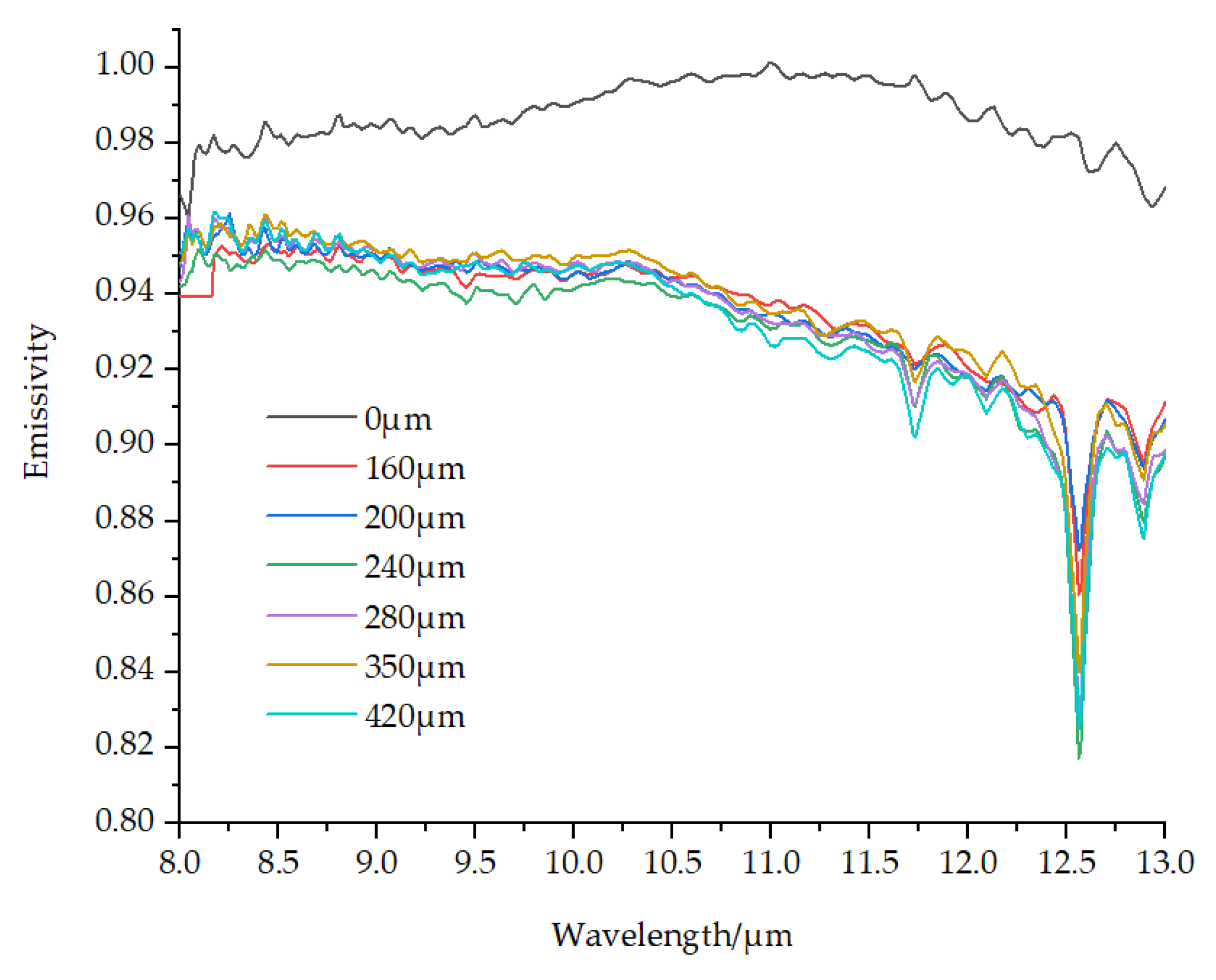
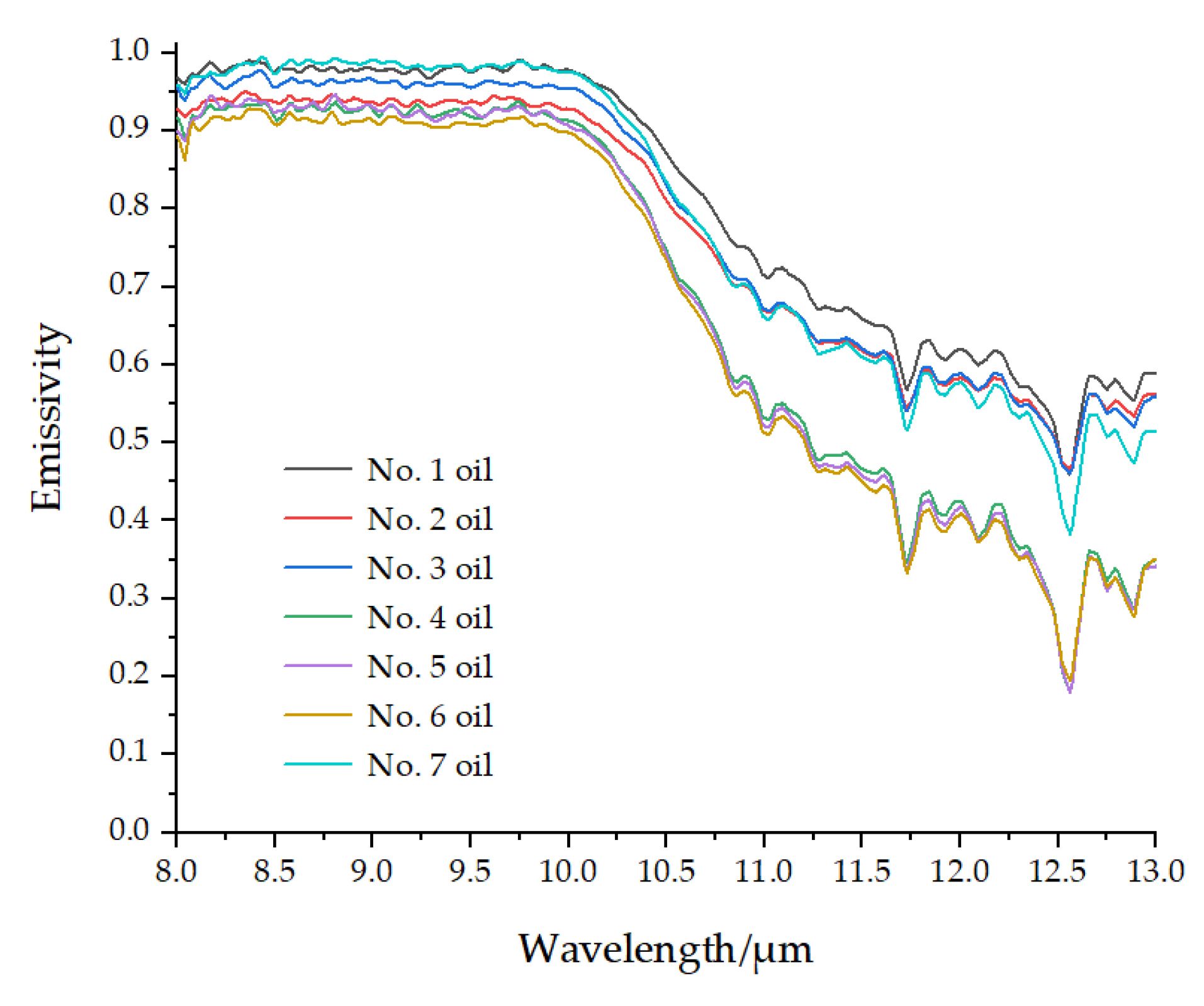
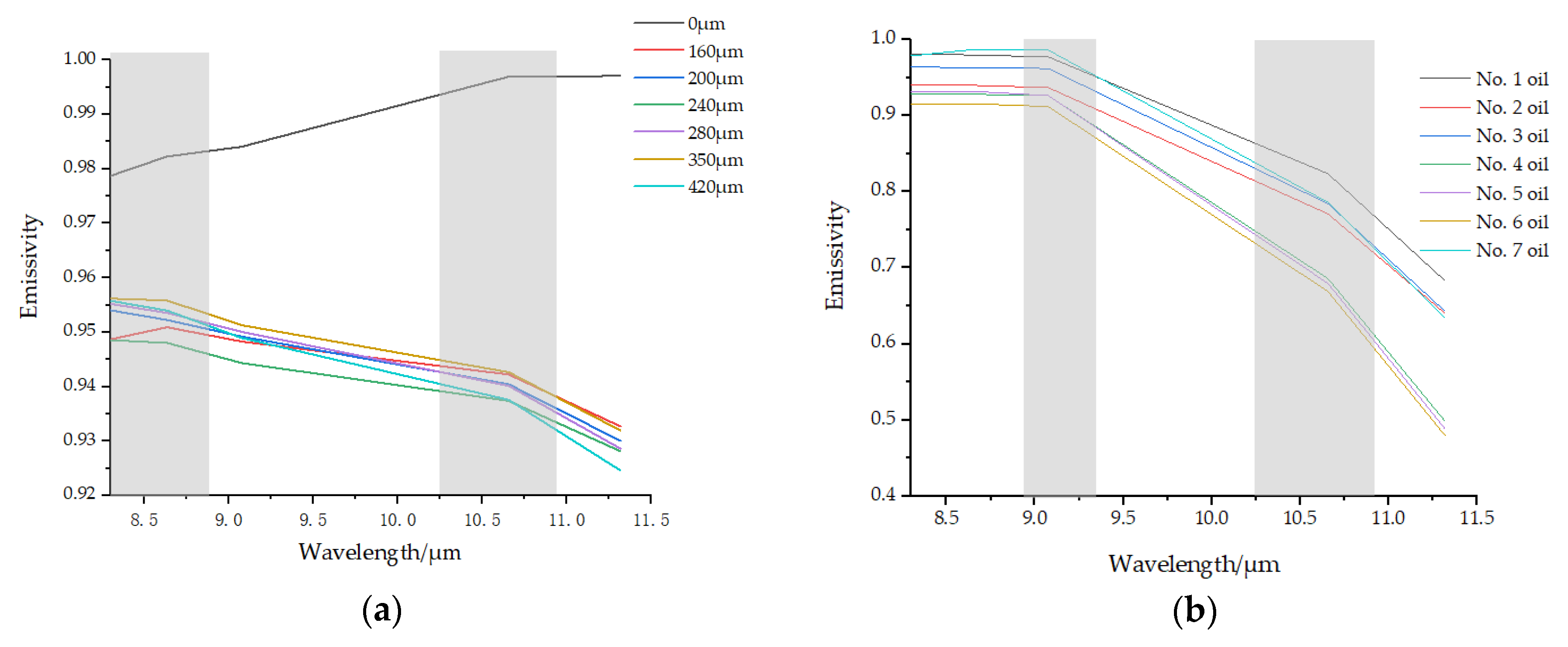
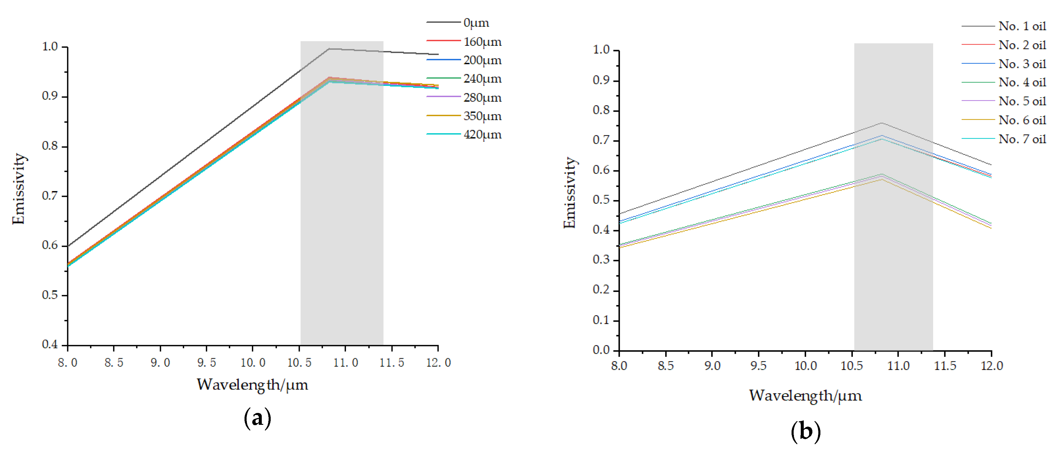
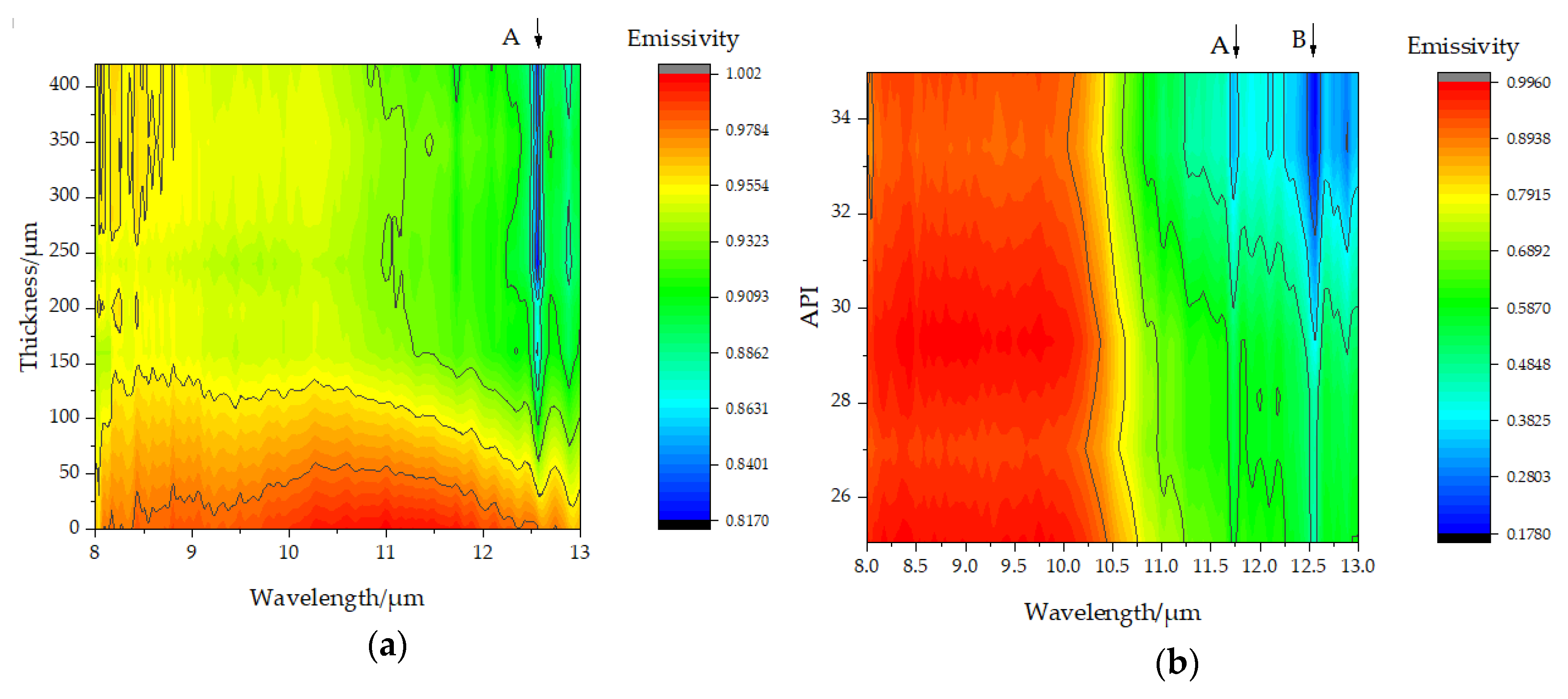
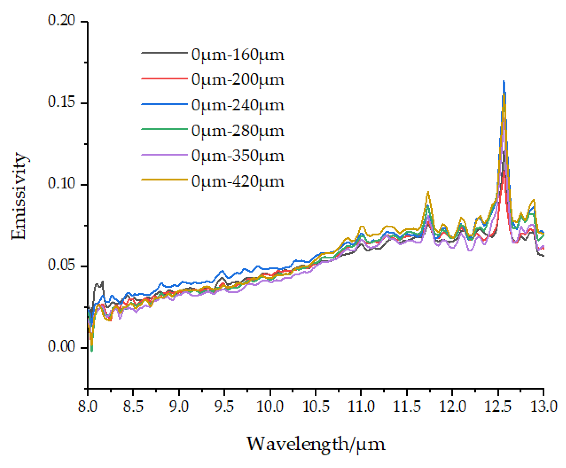
3.1. Emission Spectrum

According to analyses of oil-film spectral data, the oil characteristics became increasingly obvious with an increase in the oil film thickness. When the oil-film thickness was zero (Figure 2), the emissivity of water was measured at close to 1. Following the gradual addition of oil to the beaker, the emissivity was measured after the oil was fully diffused. As the thickness of the oil film increased, the emissivity of the oil film changed. At around 8.2 μm, the emissivity fluctuated slightly with the oil-film thickness. In the range of 8.5–10.5 μm, with the increase of oil-film thickness, the change of emissivity was small and fluctuated at around 0.95. In the range of 10.5–13 μm, the emissivity changed considerably with the oil-film thickness, and the overall emissivity showed a downward trend. Furthermore, the emissivity fluctuated considerably around 11.7 μm, 12.55 μm, and 12.8 μm. These positions are also mentioned in the research conducted by Xiong [27] and Shih [18]. According to the literature, the measured emissivity is the combination of emissivity of water and pure oil when the oil film is relatively thin. As the thickness increases, the contributions of oil become more important. The emissivity fluctuation was most obvious at 12.55 μm, where the largest reflection wave valley appeared. Here the emissivity of the oil film reached a minimum value of 0.82.

Figure 3 shows the emissivity curves of different ship fuel oils. The API is a measure designated by the American Petroleum Institute to represent the density of petroleum products. API values of different fuels are different; the larger the API value, the lighter the crude oil and the smaller the relative density. The standard temperature is 15.6 ℃ (60 °f), and its relative density at 15.6 ℃ is as follows:

$$\mathrm{API}=\frac{141.5}{\mathrm{Relative} \mathrm{density}}-131.5$$

(5)

The APIs of the fuels of the seven different ships used in this experiment are shown in Table 1.

Figure 3 shows that the trends of the wavelength emissivity curves of the fuel used by different ships were the same. However, there was a significant difference in emissivity between different fuels, whereby the emissivity of the fuel decreased with an increase in wavelength. At 8–10 μm, the emissivity (0.95) changed a little with an increase in the wavelength. However, at 10–13 μm, with the increase of wavelength, the emissivity of the fuel decreased rapidly, among which there were obvious troughs at 11.6 μm and 12.55 μm. This was the same position as the trough of the oil film in water. The lowest point of the fuel emissivity occurred at a wavelength of 12.55 μm, and the lowest value was 0.2. According to the API density of different fuel varieties, shown in Table 1, it was found that the overall trend of the emissivity curve did not change with an increase in the wavelength. However, the larger the API density, the larger the emissivity reduction range and the higher the peak value.

3.2. Cluster Analysis

The fuel classification results obtained by different ships are shown in

Table 2. Clustering results of fuel for different ships.

Stage	Cluster 1	Cluster 2	Coefficient
1	4	5	0.026
2	4	6	0.099
3	2	3	0.156
4	2	7	0.454
5	1	2	0.662
6	1	4	8.998

.

The stages in Table 2 indicate the order of clustering. Clusters 1 and 2 represent the fuel type, and clustering coefficients indicate the degree of the clustering effect. As can be seen from Figure 4, the first stage was to cluster No. 4 oil and No. 5 oil, and the clustering coefficient between the two was 0.026. Clustering was performed for No. 4 oil and No. 6 oil with a clustering coefficient of 0.099. Figure 4 shows the pedigree chart using an average join classification. The clustering results are the same as those in Table 2.

By comparing the API values of the fuel oil for each ship (Table 1), it was found that the oil with a similar API value was always clustered first and that the APIs of No. 4 oil and No. 5 oil were the closest. They were, accordingly, combined into one group in the cluster analysis. The API difference between No. 2 oil and No. 3 oil was 0.09, in which the difference was the second smallest. This was accordingly clustered in the second step in the cluster analysis. The API difference between No. 1 oil and No. 4 oil was 9.95, the largest API difference among the fuels used in the experiment. This was ultimately integrated into one group in the cluster analysis.

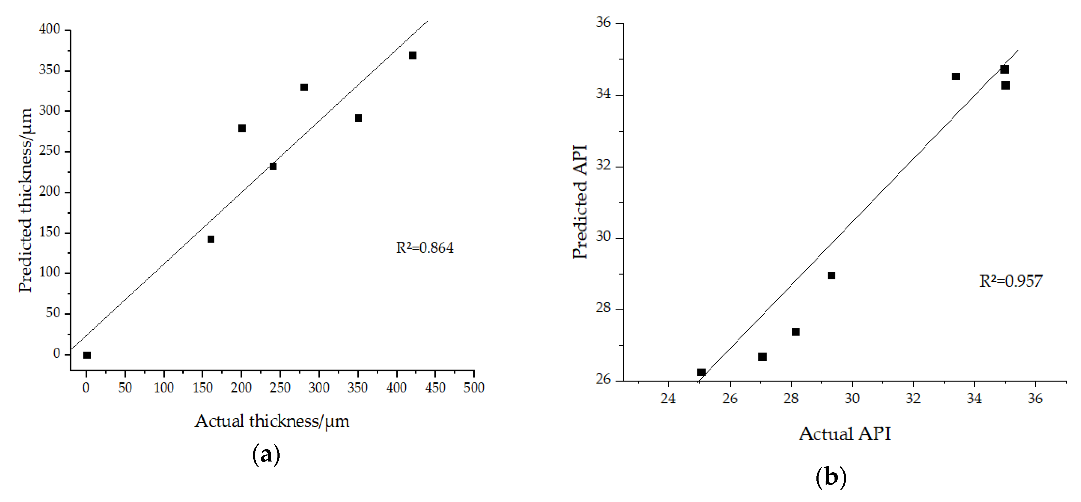
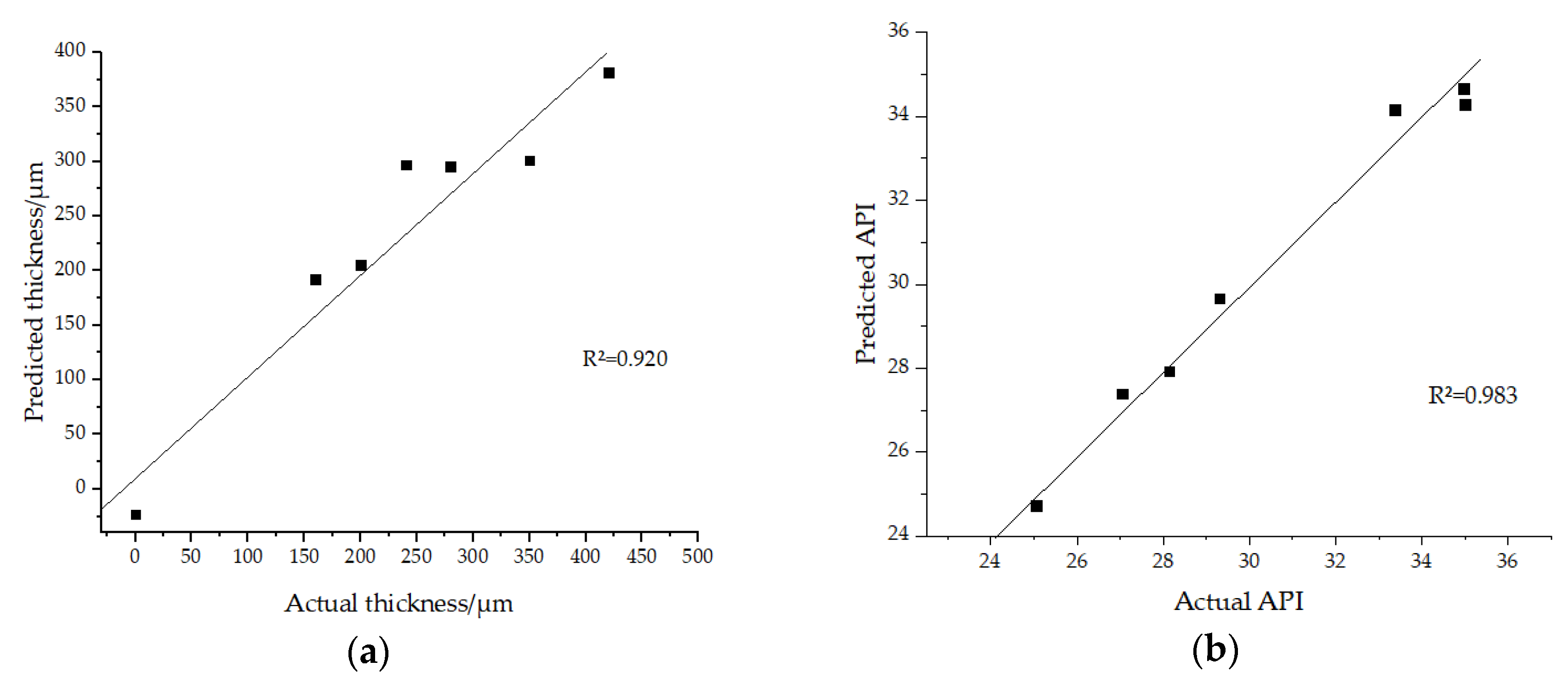
3.3. Multiple Stepwise Linear Regression

Because of the multicollinearity of the original spectral data, if the original data was used to perform multiple linear regression, the variance of the regression coefficient may be increased. At the same time, it is easy to mistake the important explanatory variable as an insignificant variable, resulting in the invalidation of the predictive function of the model. The larger variance will enlarge the prediction interval and render the prediction meaningless. The principal component analysis is a statistical correlation method for the investigation of the correlation between multiple variables. The analysis can reveal the internal structure of multiple variables through a few principal components. This analysis derives a few principal components from the original variables so that they retain as much information as possible about the original variables, and are unrelated to each other [31]. The continuum removal method can effectively highlight the characteristics of the spectral curve and normalize it to a consistent spectral background. This is advantageous for the comparison of characteristic values with other spectral curves [32]. The continuum removal method did not change the position of the sensitive wavelength, and could more effectively compare the spectral characteristic values, highlight the characteristics of the response spectrum, strengthen the characteristic shape of the spectral curve, and enhance the identifiability. Through principal component analysis and envelope curve removal, the main components of the spectral data were extracted, the dimensionality of the spectral data was reduced, and the multicollinearity was eliminated. The processed data were fitted by multiple stepwise regression, and the relationship between the predicted value and the actual value was obtained.

The principal component analysis method was used initially to reduce the dimensionality of the data. The principal component analysis was performed using SPSS (v. 25, IBM), where the variable is the emissivity at each wavelength. For the oil-film thickness emissivity data, four main components were extracted, and the cumulative contribution rate was 99.8%. Multivariate stepwise regression was used for fit modeling, and the results are shown in Figure 5a. The R² of this model is 0.864. When calculating different API fuel oil data, the principal component analysis was used to reduce the dimension of the data [25]. During the principal component analysis of different fuel emissivity data, a total of three principal components were extracted, and the cumulative contribution rate reached 99.6%. Multiple stepwise linear regression was applied to fit the fuel emissivity data of different ships and the result is shown in Figure 5b. The R² is 0.957. The models of emissivity and different oil-film thickness, and emissivity and different fuel API, all fit well.

Continuum removal of the original emissivity data with different thickness and multiple linear regression analysis was conducted on the obtained data (Figure 6a). The R² of the model is 0.920. Figure 6b shows the multiple stepwise linear regression for different API fuels after the continuum removal. The model R² is 0.983. Based on the above fitting figures, the data processed by continuum removal had a positive effect on the prediction of oil-film thickness and API density.

3.4. Thermal Infrared Sensor Data Simulation

To simulate the spectrum from airborne or spaceborne sensor images, the spectral resolution of ASTER and AVHRR was resampled [33,34]. The wavelength and full width at half maximum (FWHM) information of ASTER and AVHRR were obtained, and the spectral resampling module in ENVI (v. 5.5, Harris Corporation) used to resample the spectrum. ASTER can obtain information from visible light to the thermal infrared spectrum. It also has a range of surface image data with high geometric and radiation resolution [35,36,37]. AVHRR has high time resolution, wide-coverage, and a low price, which is useful for capturing rapid dynamic changes on the ground and is conducive to high-density dynamic remote-sensing research [38]. The data was used to resample the spectral emissivity obtained in the experiment to determine the potential for fuel detection in the thermal infrared band.

Figure 7 shows the resampling results of different oil-film thickness emissivity spectra for different satellite sensors. The resampling spectrum of ASTER (Figure 7a) shows the resampling spectrum of different oil-film thickness. According to the resamped spectrum, the oil could be separated from water easily, while the thickness of oil film could not be estimated because of the similarity of emissivity of each film. Figure 7b shows the resampling spectrum for different API fuels. It was observed that in the ASTER resampling spectrum, two frequency bands can be used to distinguish between different fuel types. The bands are band 12 (8.925–9.275 μm) and band 13 (10.25–10.95 μm). Figure 8 shows the results of the resampling of different oil-film thicknesses and different API fuels using the AVHRR. Figure 8a displays the emissivity spectra of different oil-film thicknesses convolved to the AVHRR sensor. AVHRR has two thermal infrared bands; the channel range that can be used to verify the oil-film thickness is AVHRR-4 and the wavelength range is 10.5–11.3 μm. Figure 8b shows the resampling spectrum for the emissivity of different API fuels. It was found that the AVHRR-4 could be used for oil spill detection. It has the potential to separate different oils from each other. It is quite difficult to estimate the thickness of oil film.

4. Discussion

In this experiment, the emissivities of different oil thickness and API fuel were measured. The emissivities of different fuel film thicknesses differed in the range of the thermal infrared band, and the main wave peak was between 11.5 μm and 13 μm. The position of the peak of the infrared spectrum was largely determined by the atomic mass and the chemical bond strength of the vibrating functional group [39]. Different functional groups have different atomic masses and chemical bond strengths. Therefore, different structures from the peak position of the thermal infrared spectrum can be determined.

In the measured emissivity spectrum, two distinct emissivity troughs appeared, at 11.7 μm and 12.5 μm. This is because the fuel contains a benzene ring containing aromatic bonds, which make its chemical properties and infrared spectrum unique [40]. The absorption peak position of the benzene ring was 14.7–14.9 μm, forming a single absorption band. Because the benzene ring contains six hydrogen atoms, each hydrogen atom can be replaced by other groups, so a substituted structure of the benzene ring is formed. The mono-substitution absorption position is between 12.9–14 μm. Because of the unique structure of the benzene ring, the disubstituted content is divided into m-disubstituted, o-disubstituted, and p-disubstituted. For the ortho-disubstituted, the position of the absorption peak is usually between 13–13.7 μm and the absorption diagnostic peak of the o-disubstituted is 12.3–13.3 μm. In addition, a ring-bending peak appears at 14.5 μm. There is no loop bending for the p-disubstituted, so the only absorption diagnostic peak is between 11.6 μm and 12.6 μm [41]. Because of the existence of p-disubstituted and m-disubstituted in fuel oil, the emission spectrum of p-disubstituted decreased at the wavelength of 11.7 μm, and that of m-disubstituted decreased at the wavelength of 12.5 μm.

Some experiments have used partial least square regression [42] or support vector machines [43] to establish models to predict the API density of fuel oil. In this experiment, the multiple stepwise linear regression method was used to predict the API density of fuel oil, and valuable results were obtained. At the same time, it is demonstrated that the emissivity of the fuel decreases with the increase of the API density, which confirms previous experimental results [44].

Figure 9 presents the wavelength emissivity data in the form of a contour map of different oil-film thickness and wavelength emissivity. The abscissa represents the wavelength, the ordinate represents the oil-film thickness, and the color band represents the fuel emissivity. From Figure 9a the most contour information can be observed at A, and the emissivity changes most obviously with the oil thickness. Therefore, near point A is the wavelength position (12.55 μm) where the thickness of the oil film is optimal. Figure 10 shows the difference between the emissivity of the oil film and the fuel emissivity of each oil-film thickness. From Figure 10, it can be observed that as the wavelength increased, the oil-film emissivity difference gradually increased, with the largest difference in emissivity at 12.55 μm. The maximum difference was 0.16, and a significant difference in emissivity also appeared at 11.7 μm. In conclusion, it can be seen that 12.55 μm is the optimal wavelength location for testing the fuel thickness, and 11.7 μm can also be used as the wavelength location for testing the fuel film thickness. This finding also conforms to the most sensitive region location for the fuel film thickness measured in the thermal infrared band experiment [27]. Taking the influence of atmosphere into account, the spaceborn sensors may have limited ability to distinguish oil films with different thicknesses or APIs. However, it still has the potential to separate less viscous, light oils form more viscous, heavy oils, if the hyperspectral thermal sensors are used [45]. The content of this paper will provide some reference for the thermal infrared hyperspectral spaceborne sensor to monitor oil spills in the future. In Figure 9a the ordinate represents the API value of different fuels, and the color band represents the emissivity value. From Figure 9b it is observable that in the range of 8.0–11.5 μm, as the fuel API value increased the emissivity did not change considerably, so this area cannot be used as a band to test the fuel API. As the API value increased at B, the contour line changed significantly, so B is the optimal wavelength position (12.55 μm) for testing the API value of the fuel. As the fuel API value increased at A, the fuel emissivity also changed, however, the trend is not as obvious as at B. This is also a useful wavelength position (11.7 μm) for testing the fuel API.

5. Conclusions

In this experiment, the thermal infrared spectra of different oil-film thicknesses and the thermal infrared spectra of different API fuels were measured. Multiple stepwise linear regression was used to build the model. Principal component analysis and continuum removal were used to reduce the dimensional data and reduce factor model errors due to multicollinearity. Stepwise multiple linear regression was performed using the processed data. Cluster analysis was used to cluster different types of fuels. The clustering order was based on the fuel API value. The closer the API values of the two fuels, the earlier the clustering was performed. The API values with the largest difference were merged at the end of the cluster analysis. This experiment also convolved the emissivity spectra to ASTER and AVHRR channels to assess the ability of these sensors to distinguish the oil film with different thickness and crude oil variety. The results show that the ASTER and AVHRR-4 could be used to detect oil films on the water surface. Neither of the two sensors has the ability to estimate the thickness of oil film. Bands 12 and 13 could be used to identify different types of fuel. The AVHRR-4 channel has the potential to identify different fuel types. The assessment only considered the band number and spectral response function. The influences of instrument noise, atmosphere, and the observation geometry are not taken into account. In order to obtain more accurate result, real thermal infrared remote sensing images will be used in future work to estimate the capability of sensors in oil-film detection and mornitoring.

References

1. Yang, L.; Hu, Z.; Yan, F. Threats of indicator polychlorinated biphenyls (PCBs) in six molluscs from market to food safety: A case study in Haikou City, China. Mar. Poll. Bull. 2019, 138, 187–192. [Google Scholar] [CrossRef]
2. Alves, T.M.; Kokinou, E.; Zodiatis, G.; Radhakrishnan, H.; Panagiotakis, C.; Lardner, R. Multidisciplinary oil spill modeling to protect coastal communities and the environment of the Eastern Mediterranean Sea. Sci. Rep. 2016, 6, 1–9. [Google Scholar] [CrossRef]
3. da Silva, D.A.M.; Bícego, M.C. Polycyclic aromatic hydrocarbons and petroleum biomarkers in São Sebastião Channel, Brazil: Assessment of petroleum contamination. Mar. Environ. Res. 2010, 69, 277–286. [Google Scholar] [CrossRef]
4. Lan, D.; Liang, B.; Bao, C.; Ma, M.; Xu, Y.; Yu, C. Marine oil spill risk mapping for accidental pollution and its application in a coastal city. Mar. Poll. Bull. 2015, 96, 220–225. [Google Scholar] [CrossRef]
5. Solberg, A.H.S. Remote sensing of ocean oil-spill pollution. Proc. IEEE 2012, 100, 2931–2945. [Google Scholar] [CrossRef]
6. Liu, B.; Li, Y.; Li, G.; Liu, A. A spectral feature based convolutional neural network for classification of sea surface oil spill. ISPRS Int. J. Geo-Inf. 2019, 8, 160. [Google Scholar] [CrossRef] [Green Version]
7. Liu, B.; Zhang, Q.; Li, Y.; Chang, W.; Zhou, M. Spatial–Spectral Jointed Stacked Auto-Encoder-Based Deep Learning for Oil Slick Extraction from Hyperspectral Images. J. Indian Soc. Remote Sens. 2019, 47, 1989–1997. [Google Scholar] [CrossRef]
8. Garcia-Pineda, O.; MacDonald, I.; Hu, C.; Svejkovsky, J.; Hess, M.; Dukhovskoy, D.; Morey, S. Detection of floating oil anomalies from the Deepwater Horizon oil spill with synthetic aperture radar. Oceanography 2013, 26. [Google Scholar] [CrossRef] [Green Version]
9. Sun, S.; Hu, C.; Tunnell, J.W. Surface oil footprint and trajectory of the Ixtoc-I oil spill determined from Landsat/MSS and CZCS observations. Mar. Pollut. Bull. 2015, 101, 632–641. [Google Scholar] [CrossRef]
10. Alaruri, S.D. Multiwavelength laser induced fluorescence (LIF) LIDAR system for remote detection and identification of oil spills. Optik 2019, 181, 239–245. [Google Scholar] [CrossRef]
11. Krestenitis, M.; Orfanidis, G.; Ioannidis, K.; Avgerinakis, K.; Vrochidis, S.; Kompatsiaris, I. Oil spill identification from satellite images using deep neural networks. Remote Sens. 2019, 11, 1762. [Google Scholar] [CrossRef] [Green Version]
12. Fingas, M.; Brown, C. Review of oil spill remote sensing. Mar. Pollut. Bull. 2014, 83, 9–23. [Google Scholar] [CrossRef] [PubMed] [Green Version]
13. Sun, S.; Hu, C. Sun glint requirement for the remote detection of surface oil films. Geophys. Res. Lett. 2016, 43, 309–316. [Google Scholar] [CrossRef]
14. Jing, M.; Hua, D.; Le, J. Simulation of laser induced fluorescence lidar detecting system. J. Appl. Opt. 2017, 146, 977–984. [Google Scholar]
15. Salisbury, J.W.; D’Aria, D.M.; Sabins, F.F. Thermal infrared remote sensing of crude oil slicks. Remote Sens. Environ. 1993, 45, 225–231. [Google Scholar] [CrossRef]
16. Fingas, M. The challenges of remotely measuring oil slick thickness. Remote Sens. 2018, 10, 319. [Google Scholar] [CrossRef] [Green Version]
17. Tseng, W.Y.; Chiu, L.S. AVHRR observations ofPersian Gulfoil spills. In Proceedings of the IGARSS’94–1994 IEEE International Geoscience and Remote Sensing Symposium, Pasadena, CA, USA, 8–12 August 1994; pp. 779–782. [Google Scholar]
18. Shih, W.-C.; Andrews, A.B. Modeling of thickness dependent infrared radiance contrast of native and crude oil covered water surfaces. Opt. Express 2008, 16, 10535. [Google Scholar] [CrossRef]
19. Shih, W.-C.; Andrews, A.B. Infrared contrast of crude-oil-covered water surfaces. Opt. Lett. 2008, 33, 3019. [Google Scholar] [CrossRef]
20. Niclos, R.; Dona, C.; Valor, E.; Bisquert, M. Thermal-infrared spectral and angular characterization of crude oil and seawater emissivities for oil slick identification. IEEE Trans. Geosci. Remote Sens. 2014, 52, 5387–5395. [Google Scholar] [CrossRef] [Green Version]
21. Pinel, N.; Bourlier, C. Unpolarized Infrared Emissivity of Oil Films on Sea Surfaces. In Proceedings of the 2019 IEEE International Geoscience & Remote Sensing Symposium (IGARSS 2009), Cape Town, South Africa, 12–17 July 2009; University of Cape Town: Cape Town, South Africa, 2009. [Google Scholar]
22. Xiong, P.; Gu, X.; Yu, T.; Meng, Q.; Li, J.; Shi, J.; Cheng, Y.; Wang, L.; Liu, W.; Liu, Q. Thermal infrared emissivity spectrum and its characteristics of crude oil slick covered seawater. Spectros. Spect. Anal. 2014, 34, 2953. [Google Scholar]
23. Neinavaz, E.; Darvishzadeh, R.; Skidmore, A.K.; Groen, T.A. Measuring the response of canopy emissivity spectra to leaf area index variation using thermal hyperspectral data. Int. J. Appl. Earth Obs. Geoinf. 2016, 53, 40–47. [Google Scholar] [CrossRef]
24. Ullah, S.; Skidmore, A.K.; Ramoelo, A.; Groen, T.A.; Naeem, M.; Ali, A. Retrieval of leaf water content spanning the visible to thermal infrared spectra. ISPRS J. Photogramm. Remote Sens. 2014, 93, 56–64. [Google Scholar] [CrossRef]
25. Eisele, A.; Chabrillat, S.; Hecker, C.; Hewson, R.; Lau, I.C.; Rogass, C.; Segl, K.; Cudahy, T.J.; Udelhoven, T.; Hostert, P.; et al. Advantages using the thermal infrared (TIR) to detect and quantify semi-arid soil properties. Remote Sens. Environ. 2015, 163, 296–311. [Google Scholar] [CrossRef]
26. van der Meijde, M.; Knox, N.M.; Cundill, S.L.; Noomen, F.; van der Werff, H.M.A.; Hecker, C. Detection of hydrocarbons in clay soils: A laboratory experiment using spectroscopy in the mid-and thermal infrared. Int. J. Appl. Earth Obs. Geoinf. 2013, 23, 384–388. [Google Scholar] [CrossRef]
27. Lu, Y.; Zhan, W.; Hu, C. Detecting and quantifying oil slick thickness by thermal remote sensing: A ground-based experiment. Remot. Sens. Environ. 2016, 181, 207–217. [Google Scholar] [CrossRef]
28. Yang, F.; Han, Y.; Xuan, Y. Large-scale earth surface thermal radiative features in space observation. Opt. Commun. 2015, 348, 77–84. [Google Scholar] [CrossRef]
29. Xu, J.; Meng, B.; Zhai, W.; Ding, L.; Zheng, X. Calibration of common temperature blackbody based on thermal- infrared standard radiometer. Hongwai Yu Jiguang Gongcheng/Infrared Laser Eng. 2014, 43, 716–721. [Google Scholar]
30. Liu, B.; Li, Y.; Liu, C.; Xie, F.; Muller, J.P. Hyperspectral features of oil-polluted sea ice and the response to the contamination area fraction. Sensors 2018, 18, 234. [Google Scholar] [CrossRef] [Green Version]
31. Shahdoosti, H.R.; Ghassemian, H. Combining the spectral PCA and spatial PCA fusion methods by an optimal filter. Inf. Fusion 2016, 27, 150–160. [Google Scholar] [CrossRef]
32. Li, D.; Zhi, W.; Hong, G.E. Continuum removal based hyperspectral characteristic analysis of leaves of different tree species. J. Zhejiang For. Coll. 2010, 27, 809–814. [Google Scholar]
33. Yackel, J.J.; Nandan, V.; Mahmud, M.; Scharien, R.; Kang, J.W.; Geldsetzer, T. A spectral mixture analysis approach to quantify Arctic first-year sea ice melt pond fraction using QuickBird and MODIS reflectance data. Remote Sens. Environ. 2018, 204, 704–716. [Google Scholar] [CrossRef]
34. Wettle, M.; Daniel, P.J.; Logan, G.A.; Thankappan, M. Assessing the effect of hydrocarbon oil type and thickness on a remote sensing signal: A sensitivity study based on the optical properties of two different oil types and the HYMAP and Quickbird sensors. Remote Sens. Environ. 2009, 113, 2000–2010. [Google Scholar] [CrossRef]
35. van der Meer, F.D.; van der Werff, H.M.A.; van Ruitenbeek, F.J.A.; Hecker, C.A.; Bakker, W.H.; Noomen, M.F.; Woldai, T. Multi- and hyperspectral geologic remote sensing: A review. Int. J. Appl. Earth Obs. Geoinf. 2012, 14, 112–128. [Google Scholar] [CrossRef]
36. Tomlinson, C.J.; Chapman, L.; Thornes, J.E.; Baker, C. Remote sensing land surface temperature for meteorology and climatology: A review. Meteorol. Appl. 2011, 18, 296–306. [Google Scholar] [CrossRef] [Green Version]
37. Leifer, I.; Lehr, W.J.; Simecek-Beatty, D.; Bradley, E.; Clark, R.; Dennison, P.; Hu, Y.; Matheson, S.; Jones, C.E.; Holt, B.; et al. State of the art satellite and airborne marine oil spill remote sensing: Application to the BP Deepwater Horizon oil spill. Remote Sens. Environ. 2012, 124, 185–209. [Google Scholar] [CrossRef] [Green Version]
38. Cracknell, A.P. The exciting and totally unanticipated success of the AVHRR in applications for which it was never intended. Adv. Space Res. 2001, 28, 233–240. [Google Scholar] [CrossRef]
39. Smith, B.C. IR Spectral Interpretation Workshop Why Spectral Interpretation Needs To Be Taught. Spectrosc. Springf. Eugene Duluth 2015, 30, 16–23. [Google Scholar]
40. Smith, B.C. Group wavenumbers and an introduction to the spectroscopy of benzene rings. Spectroscopy 2016, 31, 1–5. [Google Scholar]
41. Smith, B.C. Distinguishing structural isomers: Mono- and disubstituted benzene rings. Spectroscopy 2016, 31, 36–39. [Google Scholar]
42. Abbas, O.; Rebufa, C.; Dupuy, N.; Permanyer, A.; Kister, J. PLS regression on spectroscopic data for the prediction of crude oil quality: API gravity and aliphatic/aromatic ratio. Fuel 2012, 98, 5–14. [Google Scholar] [CrossRef]
43. Filgueiras, P.R.; Sad, C.M.S.; Loureiro, A.R.; Santos, M.F.P.; Castro, E.V.R.; Dias, J.C.M.; Poppi, R.J. Determination of API gravity, kinematic viscosity and water content in petroleum by ATR-FTIR spectroscopy and multivariate calibration. Fuel 2014, 116, 123–130. [Google Scholar] [CrossRef] [Green Version]
44. Correa Pabón, R.E.; de Souza Filho, C.R. Crude oil spectral signatures and empirical models to derive API gravity. Fuel 2019, 237, 1119–1131. [Google Scholar] [CrossRef]
45. Lammoglia, T.; de Souza Filho, C.R. Spectroscopic characterization of oils yielded from Brazilian offshore basins: Potential applications of remote sensing. Remote Sens. Environ. 2011, 115, 2525–2535. [Google Scholar] [CrossRef]
Figure 1. Fuel used in the experiment; Nos. 1–7 fuel and No. 0 fuel (from left to right).
Jmse 08 00135 g001
Figure 2. Emissivity data for different oil-film thickness.
Jmse 08 00135 g002
Figure 3. Emissivity data for fuel used by different ships.
Jmse 08 00135 g003
Figure 4. Cluster tree of different ship fuel oils.
Jmse 08 00135 g004
Figure 5. (a) Multiple stepwise regression image after dimension reduction by principal component analysis of emissivity data of different fuel film thickness; and (b) multiple stepwise regression image after dimension reduction by principal component analysis of emissivity data of different API fuel densities.
Jmse 08 00135 g005
Figure 6. (a) Multiple stepwise linear regression image after continuum removal of different fuel film thicknesses; and (b) multiple stepwise linear regression image after continuum removal of different API fuel densities.
Jmse 08 00135 g006
Figure 7. (a) Resampling spectra of the fuel film thickness emissivity using Advanced Spaceborne Thermal Emission and Reflection Radiometer (ASTER); and (b) resampling spectra of the emissivity of different API fuel densities using ASTER.
Jmse 08 00135 g007
Figure 8. (a) Resampling spectra of fuel film thickness emissivity using Advanced Very High Resolution Radiometer (AVHRR); and (b) resampling spectra of emissivity of different API fuel densities using AVHRR.
Jmse 08 00135 g008
Figure 9. Contour maps of (a) different fuel film thickness and wavelength emissivity; and (b) API fuel density and wavelength emissivity for different fuels.
Jmse 08 00135 g009
Figure 10. Difference between water emissivity and emissivity of each oil-film thickness.
Jmse 08 00135 g010