Identifying the Frequency Dependent Interactions between Ocean Waves and the Continental Margin on Seismic Noise Recordings

Abstract

This study presents an exploration into identifying the interactions between ocean waves and the continental margin in the origination of double-frequency (DF, 0.1–0.5 Hz) microseisms recorded at 33 stations across East Coast of USA (ECUSA) during a 10-day period of ordinary ocean wave climate. Daily primary vibration directions are calculated in three frequency bands and projected as great circles passing through each station. In each band, the great circles from all stations exhibit largest spatial density primarily near the continental slope in the western North Atlantic Ocean. Generation mechanisms of three DF microseism events are explored by comparing temporal and spatial variations of the DF microseisms with the migration patterns of ocean wave fronts in Wavewatch III hindcasts. Correlation analyses are conducted by comparing the frequency compositions of and calculating the Pearson correlation coefficients between the DF microseisms and the ocean waves recorded at selected buoys. The observations and analyses lead to a hypothesis that the continental slope causes wave reflection, generating low frequency DF energy and that the continental shelf is where high frequency DF energy is mainly generated in ECUSA. The hypothesis is supported by the primary vibration directions being mainly perpendicular to the strike of the continental slope.

1. Introduction

Ambient noise (or seismic noise) has been widely used to estimate the seismic site effect parameters (e.g., predominant frequency f₀, sediment thickness, amplification factor, etc.) of a site [1,2,3,4,5] and to characterize both deep (down to the mantle of the Earth) and shallow (within the depth of geological engineering activities) subsurface structures [6,7,8,9,10,11,12,13,14,15] for its advantages as a fast, effective, and reliable tool. However, the accuracies and reliabilities of the applications listed above would be strongly affected by the spatial and temporal variations of the ambient noise sources. One example is given in [16] who estimated the amplification factors in Northern Mississippi of United States applying the horizontal-to-vertical spectral ratio (HVSR, or Nakamura) method based on long term ambient noise recordings. As the f₀s in their study region lie in the frequency band of ocean waves induced double-frequency (DF) microseisms (0.1–0.5 Hz), the estimated amplification factors (HVSR values at f₀) fluctuate with time and are strongly correlated with the energy of the DF microseisms as well as the ocean wave height. Many other studies suggest that if the noise sources are not homogeneously distributed, the cross-correlation function cannot be reconstructed causing big errors in subsurface tomography or even failure of subsurface tomography [17,18,19,20,21,22]. In addition, the ambient noise with frequency greater than 0.1 Hz would be used in shallow subsurface tomography. From this point of view, exploring the source locations, the spatial and temporal characteristics and the generation mechanisms of the ambient noise with frequency greater than 0.1 Hz, especially the DF microseisms, would significantly improve the application of the ambient noise in site effect evaluation and shallow subsurface tomography.

In the spectrum of ambient noise recorded globally, the DF microseisms (or secondary microseisms) manifest themselves as one or more energy peaks in the frequency band of 0.1–0.5 Hz which is roughly twice of ocean waves’ frequencies. It is widely accepted that DF microseisms are generated by the nonlinear interaction between ocean waves propagating in opposite directions with similar frequencies (e.g., [23,24,25,26,27,28,29,30,31]).

Recent studies suggest that two different circumstances may be responsible for generating opposing ocean waves that trigger DF microseisms. The first group considers wave–wave interactions in the open-ocean during strong storms [27,32,33,34]. However, DF microseisms can be observed worldwide even when there are no strong storms locally or globally. This is explained by the second group of studies who emphasize the role of interactions between the incident and reflected ocean waves at the continental margin [22,35,36,37,38,39]. For example, the authors of [40] observed that Rayleigh waves in a microseism recording at an ocean bottom seismometer in the Pacific Ocean were approaching from California coast during a super-typhoon rather than the location of the typhoon and concluded that the microseisms were generated by interactions of typhoon-induced waves toward and their reflections from the coastal line. In a different set of studies based on correlation analyses between the ocean storms developed close to shorelines and the ambient noise recorded on coastal seafloor or costal land, it was recognized that the long- and short-period DF microseisms (LPDF, 0.1–0.2 Hz and SPDF, 0.2–0.5 Hz, respectively) were excited by swells from distant and local waves, respectively [25,30,31,41,42]. However, regarding the locations where the interactions (reflection) occur, there exist a debate in terms of the water depth (deep or coastal). In [43] the authors summarized the debate and compared theoretical and observed DF characteristics for each case considering the ocean wave frequency composition and velocities. It appears that the relationship between DF microseisms and ocean waves is not yet directly investigated as a function of water depth across the continental margin.

In this study, the continental slope, as a boundary between shallow (continental shelf) and deep (open ocean) water, is explored for its interactions with the ocean waves as well as its role and significance in the generation of DF microseisms. To reach this goal, a total of 10-days (2014/325–334) of ambient noise recordings the WAVEWATCH III^® (WWIII) hindcasts of ocean wave energy in Atlantic Ocean, and ocean wave climate parameters are utilized and analyzed.

2. Materials and Methods

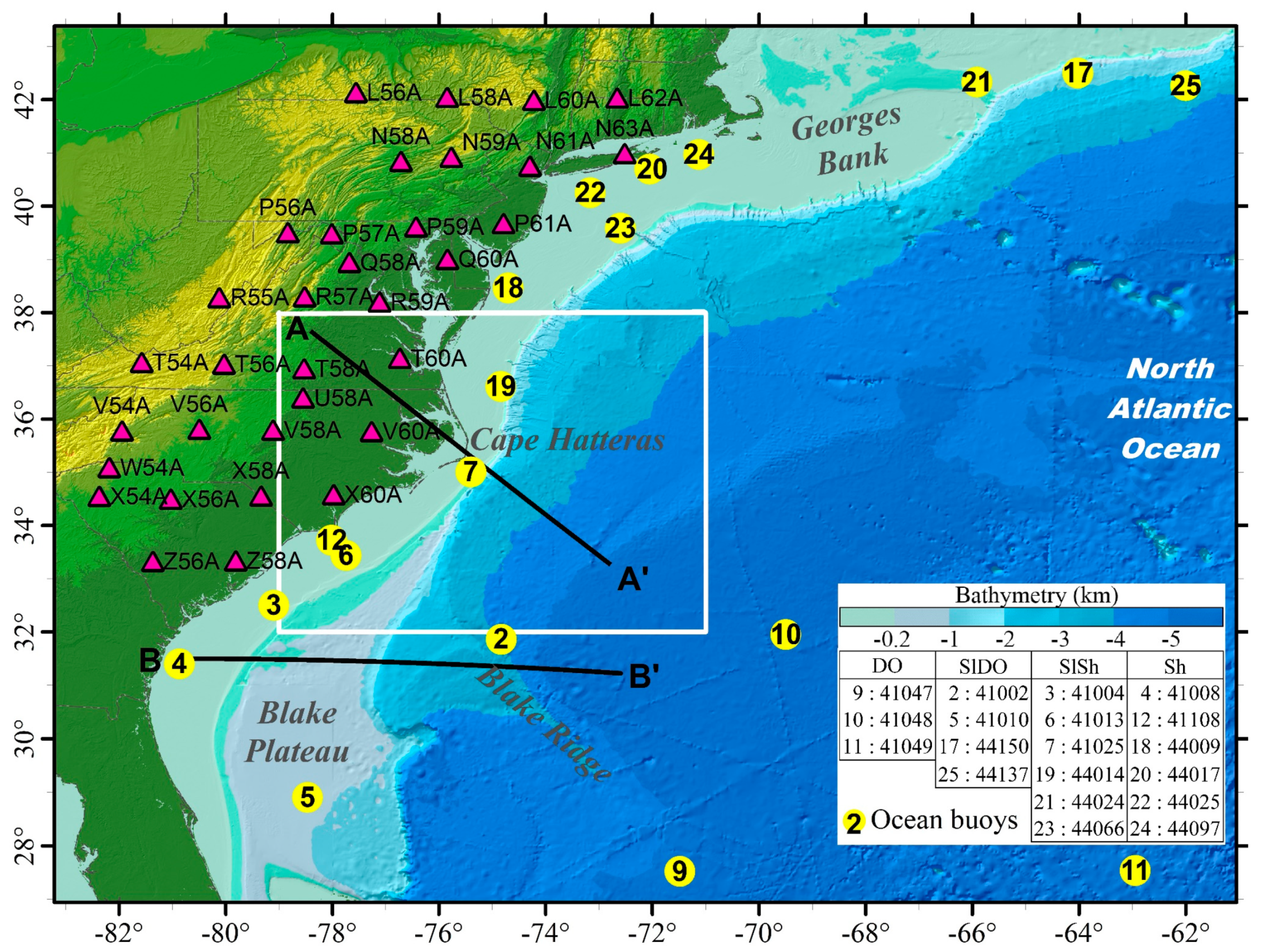
2.1. Ambient Noise Data

The selected ambient noise data were recorded at 33 broadband seismic stations (Figure 1, see IRIS Data Management Center for further details of the instruments) of the Transportable Array (TA) network along parts of the middle and southeastern North Atlantic coastal area and the Shenandoah Valley. The original time series of amplitude in vertical (V), north-south (N), and east-west (E) directions archived with a sampling rate of 40 samples-per-second were first parsed into 1-h segments, followed by removing the mean, linear trend, and instrument response in each segment [44]. Then each segment was processed following a 14-step procedure summarized below, to estimate the power spectral density (PSD) in vertical (V) direction (steps 1–4), and the primary vibration direction by the radial-to-transverse spectral ratio (Ra) method (steps 5–9) as well as the polarization analysis method based on [45] (steps 10–13) in the three DF bands (DF1, 0.1–0.2 Hz; DF2, 0.2–0.3 Hz; and DF3, 0.3–0.4 Hz). The two methods used to estimate the primary vibration directions are both based on an assumption that DF microseisms propagate dominantly as a fundamental mode Rayleigh wave [34,46,47,48]. The Ra method searches the direction of the largest ratio of radial to transverse components on the horizontal plane which is expected to be along the propagation direction of a Rayleigh wave [29,44]. The polarization analysis method represents the particle motion within a short time range (when the propagation direction is reasonably stable) as an ellipsoid with three axes perpendicular to each other [45], from which the back azimuth of the major axis with highest probability for the whole recording period can be calculated. If the primary energy source is stable and strong enough, and significantly larger than secondary sources, the primary vibration directions obtained by the two methods would agree because the secondary sources do not alter the direction of the major axis but increase the Ra values in directions other than the major axis.

The steps of the data analysis are:

(1)

Apply an anti-triggering algorithm based on a prescribed range of short (1 s) to long (30 s) term average amplitude ratios (0.2 < STA/LTA < 2.5) to filter each segment for avoiding occasional energy bursts [4,50].

(2)

Apply fast Fourier transform with a 10% cosine taper on the filtered segments in three directions to calculate spectra ($V\left(f\right)$, $N\left(f\right)$, and $E\left(f\right)$) and then smooth them using Konno–Ohmachi method with a bandwidth coefficient of 40 [51].

(3)

Compute the PSDs in the vertical direction [52] in the unit of (m/s²)²/Hz dB:

$$PSD\left(f\right)=10\log \left[\frac{1}{0.825}·\frac{2\Delta t}{N}·V{\left(f\right)}^2\right]$$

(1)

where $\Delta t$ is the sample interval (0.01 s); N is the number of samples in each selected time-series segment; the constant 1/0.825 is a scale factor to correct for the 10% cosine taper applied [53].

(4)

Plot the PSDs of all segments at each station in time-frequency domain $PSD\left(t,f\right)$.

(5)

Apply band-pass filter using the frequency bands, F = 0.1–0.2 Hz (DF1), 0.2–0.3 Hz (DF2), and 0.3–0.4 Hz (DF3) to each 1-h segment to produce filtered amplitude-time series $V\left(t,F\right)$, $N\left(t,F\right)$, and $E\left(t,F\right)$.

(6)

Rotate the two horizontal components by an angle φ into radial (R) and transverse (T) components [54] in each segment:

$$\left[\begin{array}{c}R\left(t,F,\phi \right)\\ T\left(t,F,\phi \right)\end{array}\right]=\left[\begin{array}{cc}-\cos \left(\phi \right)& -\sin \left(\phi \right)\\ -\sin \left(\phi \right)& -\cos \left(\phi \right)\end{array}\right]\left[\begin{array}{c}N\left(t,F\right)\\ E\left(t,F\right)\end{array}\right]$$

(2)

in which φ is defined as the back-azimuth angle between the north and the radial direction from the recording station toward the source.

(7)

Calculate the root mean square of $R\left(t,F,\phi \right)$ and $T\left(t,F,\phi \right)$ in each segment and their ratio $Ra\left(F,\phi \right)$.

(8)

Repeat steps 6 and 7 to calculate $Ra\left(F,\phi \right)$ at every 1° increment of angle φ in 1°–360°.

(9)

Calculate average values of $Ra\left(F,\phi \right)$ for all segments at a station and determine the azimuth ${\phi }_m$ for the maximum value of these averages. The angle ${\phi }_m$ is taken as the primary vibration direction by $Ra$ method.

(10)

Further parse the filtered 1 h segments in step 6 into ten 120 s windows and determine $V_{ij}$, $N_{ij}$, $E_{ij}$, where i = 1, 2, and 3 (separating DF1, DF2, and DF3 contents) and j = 1, 2, …, 30 (number of windows). For each window, build the three-component covariance matrix M:

$$M_{ij}=\left[\begin{array}{ccc}cov\left(V_{ij},V_{ij}\right)& cov\left(V_{ij},N_{ij}\right)& cov\left(V_{ij},E_{ij}\right)\\ cov\left(N_{ij},V_{ij}\right)& cov\left(N_{ij},N_{ij}\right)& cov\left(N_{ij},E_{ij}\right)\\ cov\left(E_{ij},V_{ij}\right)& cov\left(E_{ij},N_{ij}\right)& cov\left(E_{ij},E_{ij}\right)\end{array}\right]$$

(3)

(11)

Calculate the three eigenvalues ${\lambda }_{ij}$ and associated eigenvectors ${\overrightarrow{x}}_{ij}$ of the covariance matrix $M_{ij}$ by solving:

$$M_{ij}{\overrightarrow{x}}_{ij}={\lambda }_{ij}{\overrightarrow{x}}_{ij}$$

(4)

and define the maximum eigenvalue ${\lambda }_{ij1}$, and associated eigenvectors ${\left(\begin{array}{ccc}{x}_{i{j}_{11}}& x_{i{j}_{12}}& x_{i{j}_{13}}\end{array}\right)}^{⊺}$.

(12)

Find the back azimuth angle ${\phi }_{ij}$ corresponding to the major axis of the polarized ellipse:

$$\{\begin{array}{cc}{\phi }_{ij}=\arctan \frac{x_{i{j}_{13}}}{x_{i{j}_{12}}}& \mathrm{if} x_{i{j}_{11}}>0\\ {\phi }_{ij}=\arctan \frac{x_{i{j}_{13}}}{x_{i{j}_{12}}}+180& \mathrm{if} x_{i{j}_{11}}<0\end{array}$$

(5)

Compute the probability of the back azimuth angle within 0°–360° range with a 10° bin width. The back azimuth of highest probability is considered as the primary vibration direction by the polarization method.

2.2. Ocean Data

Theoretically, the frequencies of ocean waves that generate DF microseisms should be half of the frequencies of DF peaks. Therefore, daily WWIII hindcast of E(F/2) (log10(m²/Hz)) distributions within the half frequency bands of corresponding DF peaks are used in this study in order to explore the association between the ocean wave climates in Northern Atlantic Ocean and DF microseisms.

Additionally, a total of 19 ocean buoys in Atlantic Ocean (see Figure 1 for locations) were selected to retrieve recordings of the ocean climate parameters including dominant wave period and significant wave height (detailed descriptions of which can be found at National Data Buoy Center website). In order to clearly display the locations of the buoys on the figure and to facilitate discussion of the observations, these buoys were renumbered and divided into four groups according to their locations (Figure 1): (1) deep ocean (DO) buoys (9, 10, and 11); (2) the continental slope and deep ocean side (SlDO) buoys (2, 5, 17, and 25); (3) the continental slope and shelf side (SlSh) buoys (3, 6, 7, 19, 21, and 23); and (4) the continental shelf (Sh) buoys (the remaining ones).

In order for a direct comparison of frequency compositions of the ocean wave and DF microseisms, the dominant ocean wave frequency of ocean waves at each buoy was simply doubled to determine the double ocean wave frequency (DWF).

2.3. Source Regions of DF Microseisms

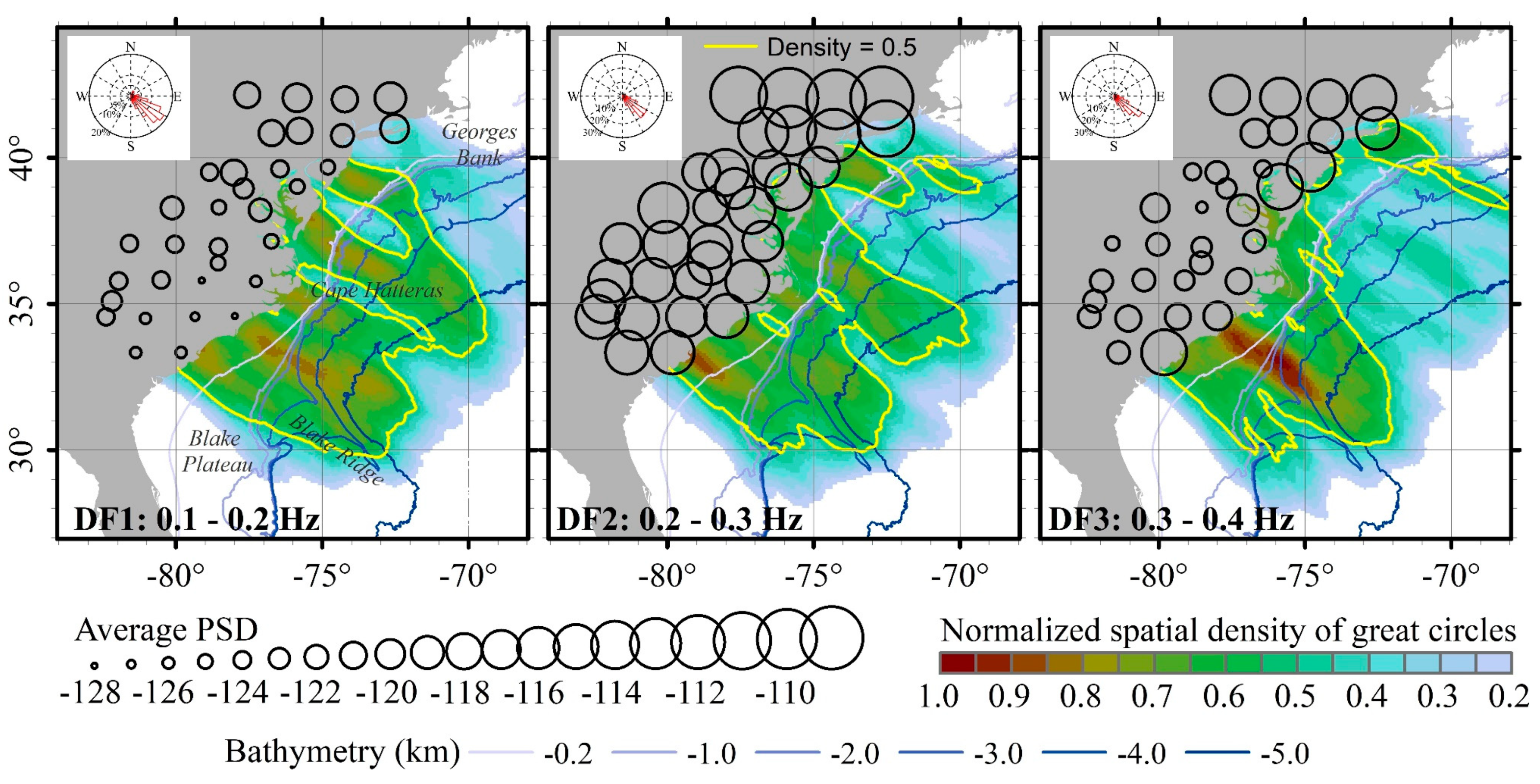
2.3.1. Spatial Density of Primary Vibration Directions

The daily primary vibration directions (${\phi }_{m1}$) were calculated for all stations and the great circles corresponding to all ${\phi }_{m1}$ were generated in the three DF bands. Any point on a great circle can be considered as a possible energy source of the corresponding station in the corresponding day and DF band. In order to find the possible source areas, spatial density of the points sampled from the great circles with a sampling interval of 100 m were calculated, normalized, and plotted as a color gradient map for each DF band. The relative magnitude of the spatial density reflects the possibility of the area to be an energy source, i.e., the larger the density, the higher the possibility.

2.3.2. Correlation Analyses

As the selected recording period was free of major anomalous ocean activities (e.g., ocean storm, typhoon, hurricane) in Atlantic or Pacific Oceans (according to National Hurricane Center, NHC), the DF microseisms were generated by the interactions of the incoming ocean waves and those reflected at the continental margin. In order to investigate the significance of the continental slope in the excitation of the DF microseisms quantitatively under normal sea states, correlation analyses of time histories between DF microseisms and ocean wave energy were carried out by considering the time-dependent variation of frequency composition and energy levels. A few DF microseism events were identified as their PSD levels are higher than the average PSDs in the whole recording period in the frequency band. Their generation mechanisms were explored by comparing temporal and spatial variations of the PSDs to the migration patterns of ocean wave fronts in WWIII hindcasts in corresponding frequency bands, as well as comparing the frequency band of each event to the DWF of ocean buoys in four groups. For the entire period of microseism recordings, Pearson correlation coefficients (CC) were calculated between the DF microseisms and ocean wave heights recorded at selected buoys in each frequency band.

3. Results

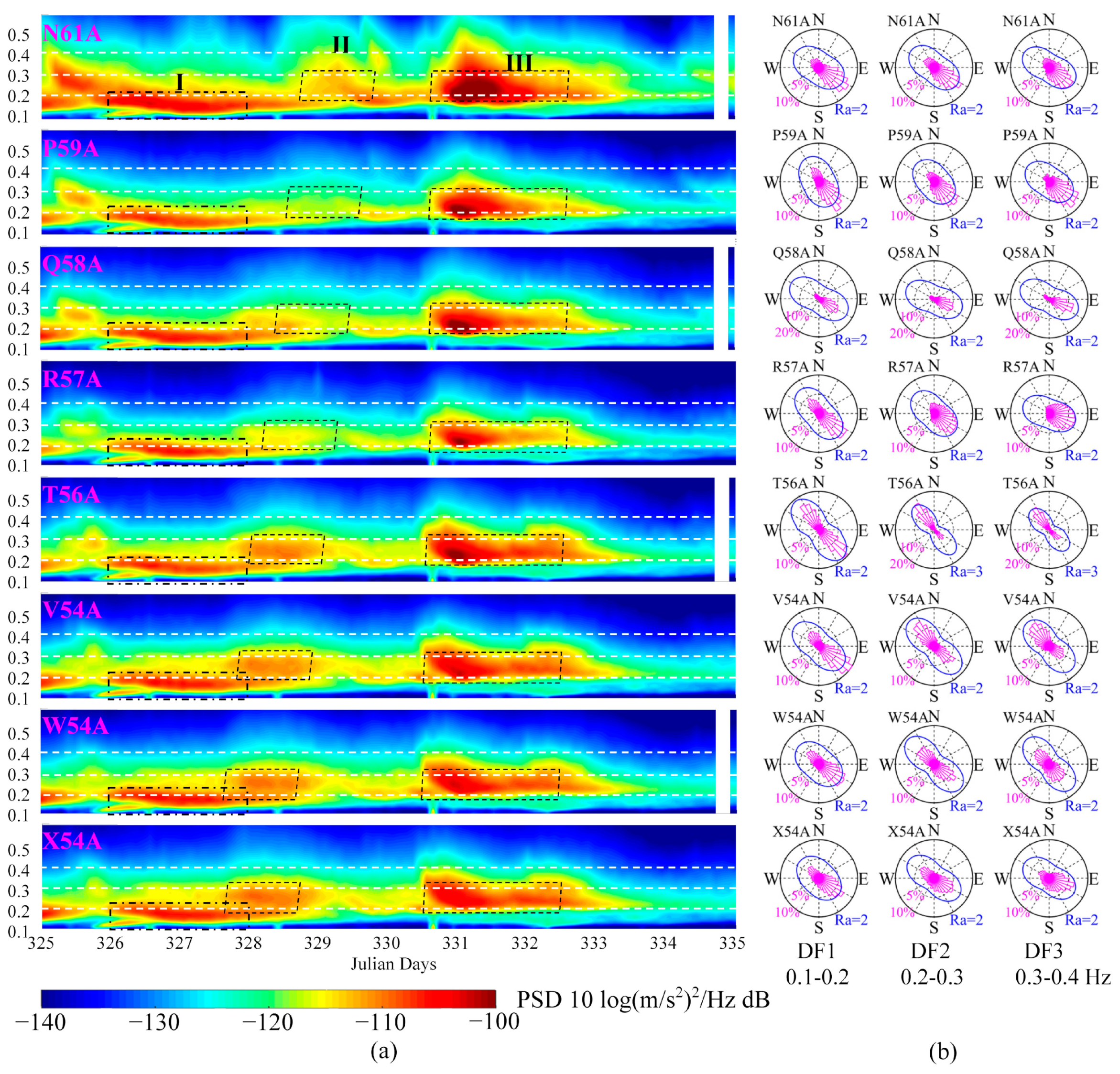
3.1. Power Spectral Density (PSD)

Figure 2a shows the vertical PSD(t,f) plots at the stations selected to cover a wide latitude range (40°N–34°N) (see Figure 1 for locations of the stations). The remaining stations were divided into three groups according to their locations (for their groups, see Figure S1a in the Supplementary Materials to this article) and their $PSD\left(t,f\right)$ plots are shown in Figure S1b,d,f. In the recording time period of this study, DF peaks are mainly in the frequency band of 0.15–0.3 Hz at the selected example stations, however, may cover a much wider frequency band at the stations close to the coastline (see Figure S1b in the Supplementary Materials to this article). At all stations, three DF microseism events are identified and labeled with I, II, and III which will be described in Section 3.3.

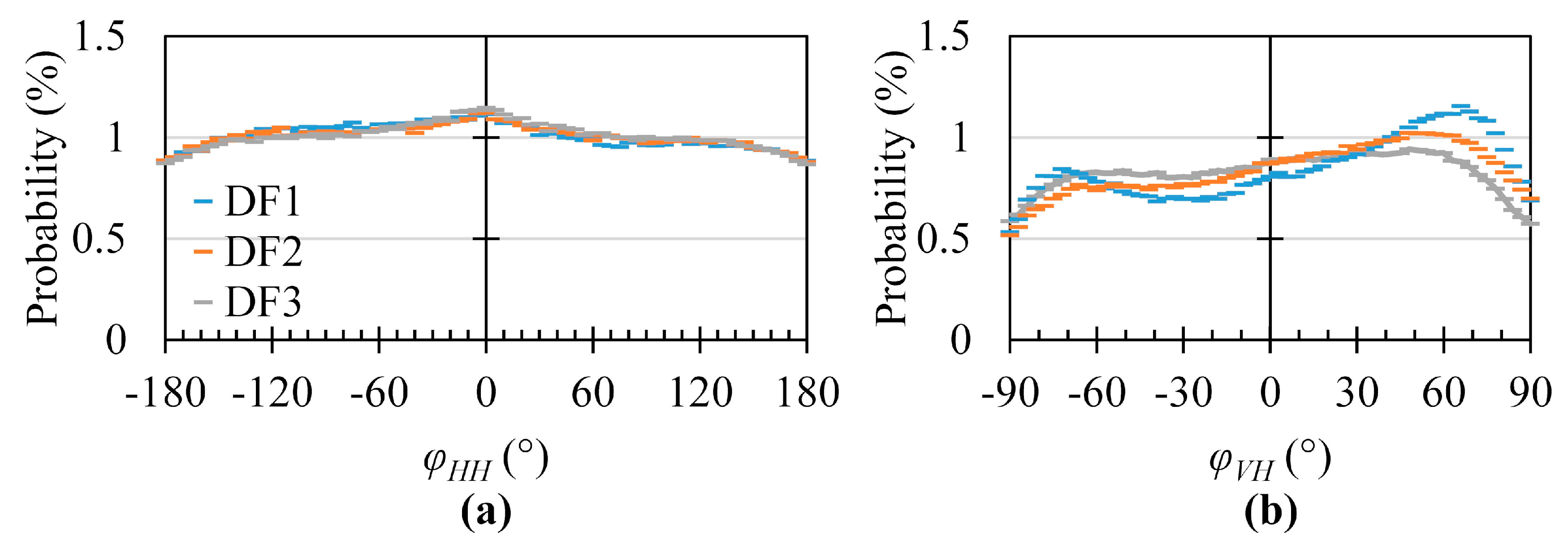
3.2. Primary Vibration Directions at DF Peaks

Figure 2b presents the polar plots of average radial-to-transverse spectral ratios Ra(φ) (blue outline) and rose diagrams of back azimuths calculated by the polarization analysis (purple) in DF1, DF2, and DF3 bands for the selected stations over the entire recording period of 10 d. The same plots for the remaining stations are given in Figure S1c,e,g in the Supplementary Materials. The longer axis of each $Ra\left(\phi \right)$ outline is identified indicating the average primary vibration direction in 10 days (${\phi }_{m10}$), which closely coincide with the major polarized direction.

The ${\phi }_{m1}$s was calculated as well for all stations, and rose diagrams of them in 10 days were generated for the three DF bands in Figure 3. The main back-azimuth in the three DF bands are shown to be in 110°–150°, which is perfectly consistent with the results in the same area in [55].

The spatial density of ${\phi }_{m1}$s was calculated, normalized, and plotted as a color gradient map for each DF band in Figure 3, as well as the contours at a density of 0.5 and the ocean bathymetries. Comparing the three maps, it can be observed that the areas of high spatial density, e.g., the areas sketched by the density contours of 0.5, shrink towards the continental shelf with increase of frequency, and the spatial density in the area between Blake Ridge and Cape Hatteras is high in all three DF bands.

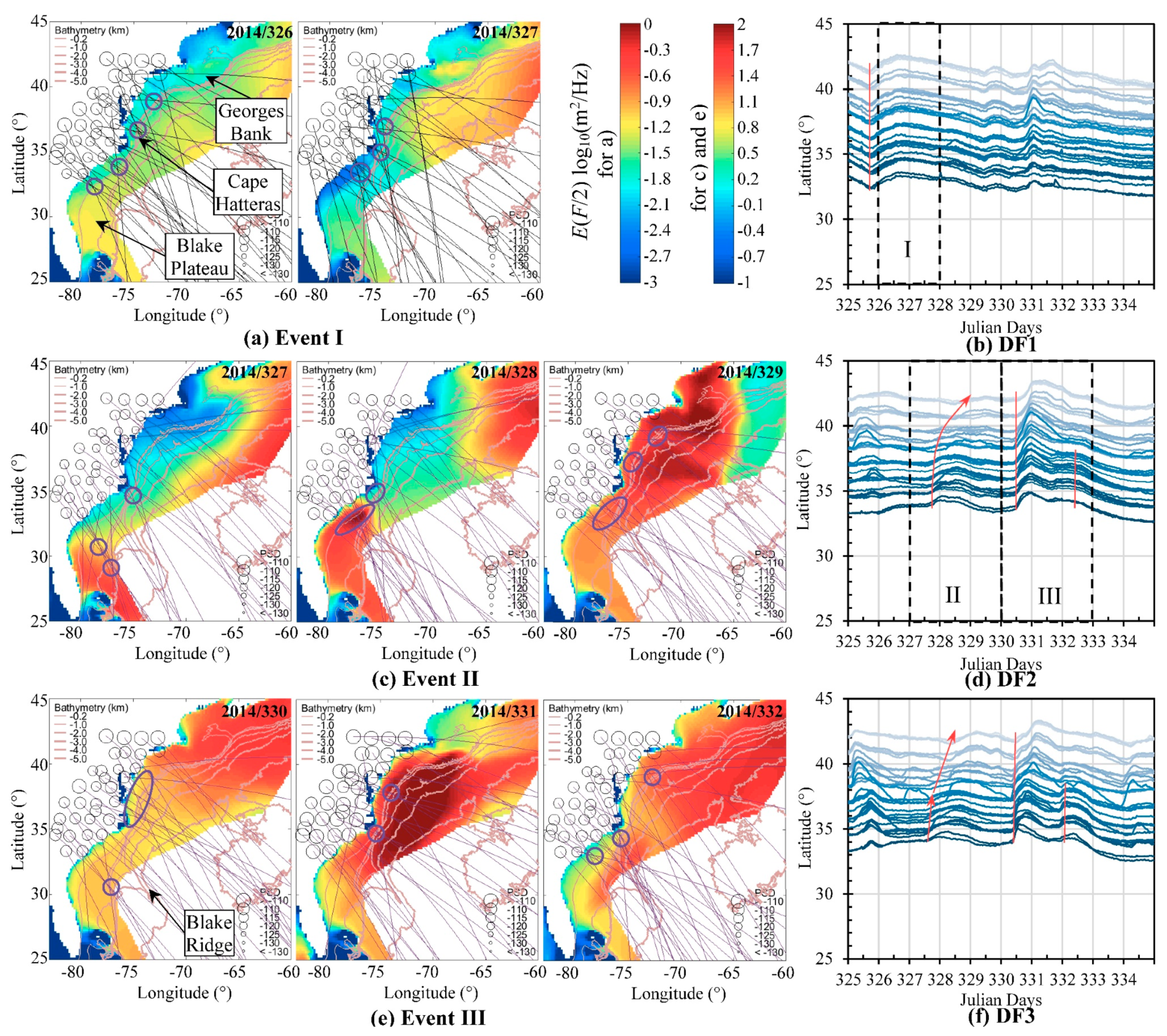
3.3. Excitation of the Three Relatively Strong DF Microseism Events

First, the spectral WWIII hindcasts of ocean wave energy (E(F/2) in log10(m²/Hz)) in North Atlantic Ocean (see Figure S2 in the Supplementary Materials to this article) were used to explore the temporal and spatial relationships in each frequency band of the energy levels between PSDs and wave energy. This result demonstrates that (1) the primary vibration directions do not point to the areas of high wave energy in open ocean, and (2) variations of ocean wave activities in open ocean of the North Atlantic Ocean have limited influence on the DF microseisms observed in the east coast of the United States.

Based on the spatial density of great circles of ${\phi }_{m1}$s presented in Figure 3, it can be inferred that the excitations of DF microseisms appear to be associated with the ocean waves in different areas of the continental margin of the western North Atlantic Ocean. Therefore, the excitation mechanisms of the three DF microseism events identified in Figure 2 are explored below with reference to the area of the continental margin as outlined in Figure 4.

Figure 4a,c,e shows the WWIII hindcasts of E(F/2) in the western Northern Atlantic Ocean (color gradient maps) within the half frequency band of events I, II, and III identified in Figure 2. In the corresponding days and frequency bands of the events, the PSD levels and the primary vibration directions are demonstrated by the small circles with scaled sizes and segments of great circles passing though the corresponding stations. The bathymetries of the western Northern Atlantic Ocean are plotted as well in order to examine the importance of the continental slope in generation of DF microseisms. In Figure 4b,d,f, the arrival times of each event are picked on the PSD-time plots of all stations, and the connection of them form the red lines indicating the sequence of energy impact on stations. In order to facilitate the description of the spatial variations of PSD levels and primary vibration directions, the area where stations are placed are divided into two sections, north and south of Cape Hatteras.

3.3.1. Event I

The energy of event I in DF1 band (LPDF, 0.1–0.2 Hz) starts to appear in late hours of day 2014/325 (red line on day 325 in Figure 4b) and reaches a higher strength on days 2014/326 and 327 (Figure 2 and Figure 4b). The ocean waves in frequency band of 0.05–0.1 Hz in the deep ocean close to the continental slope are uniformly higher on day 326 than day 327, and extend to the continental slope (Figure 4a). In addition, intersections of great circles concentrate at several small areas (purple circles) evenly distributed on the continental slope on day 326. All these observations might explain the occurrence of event I at the same time on day 326. The ocean wave energy decreases in the deep ocean close to the continental slope and increase slightly at the deep ocean area south of Georges Bank on day 327. The primary vibration directions at all stations cover a wider range, and the intersections of great circles are not as concentrated as on day 326. These changes can explain the decrease of PSD levels at most stations except for eight northernmost stations on day 327.

3.3.2. Event II

The event II in DF2 (0.2–0.3 Hz) band occurs on days 2014/327, 328, and 329, and arrives at the stations in south section before north section as indicated by the curved red arrow in Figure 4d. This sequence can be explained by the ocean wave interactions associated with the continental slope (Figure 4c).

On day 327, the wave energy in frequency band of 0.1–0.2 Hz is relatively higher on lower Blake Plateau (water depth 200–2000 m) and many great circles of the stations in the south section intersect on the edge of this area. The PSD levels at the stations in the south section are roughly proportional to their distances to lower Blake Plateau. Then on day 328 the wave front moves north along the continental slope to south of Cape Hatteras while the wave energy increases to the highest. The great circles of almost all stations in south section intersect in this area, and the PSD levels at these stations increase significantly. On day 329, the wave front moves further north to the area between Georges Bank and Cape Hatteras where the strike of the continental slope turns almost 90°, causing the significant increase of wave energy in this area. The great circles at the stations in north section do not intersect in the open ocean where the wave energy is higher, but on the continental slope segments south of Georges Bank and north of Cape Hatteras. The PSD levels at the stations to the north increase but not as significantly as at the southern stations on day 328. The great circles at the southern stations still intersect at the continental slope between Cape Hatteras and Blake Plateau but not as concentrated as on day 328.

3.3.3. Event III

The event III in DF2 (0.2–0.3 Hz) band occurs on days 2014/330, 331, and 332, arrives at the stations almost at the same time, but generates the energy peaks slightly earlier at the stations in the south section (Figure 4d). This sequence can also be explained by the ocean wave interactions associated with the continental slope (Figure 4e).

On day 330, the great circles of most stations point to the area between Georges Bank and Blake Plateau where the ocean waves are roughly the same height, and intersect evenly on this continental slope segment. However, the ocean wave energy on the continental slope of Georges Bank are relatively higher which coincide well with the relatively higher PSD levels at the four northernmost stations. On day 331, the ocean wave energy grows very fast while the wave front moves north quickly to Georges Bank, resulting in high waves on the continental slope segment and deep ocean area between Georges Band and Blake Ridge. Most intersections of the great circles align on this continental slope segment and nearby deep ocean, and the PSD levels are very high at all stations. On day 332, the wave front moves to northeast of Georges Bank and the wave energy decreases moderately. However, the wave energy on the continental slope south of Georges Bank is still relatively high and many great circles of the stations in northern section intersect here, which might be the reason for high PSD levels at the eight northernmost stations. A new high wave front is developed at Blake Ridge where most great circles of stations in southern section intersect, and a new PSD peak appears at the stations in the southern section.

3.4. Correlation between DF Microseisms and Ocean Wave Parameters

The time histories of average PSDs in DF1, DF2, and DF3 bands are shown in Figure 4b,d,f, respectively. The curves are stacked according to the latitudes of the stations and the reliefs show the time-dependent variations of PSD levels. The DWFs at the DO, SlDO, and SlSh buoys are closer to the frequency band of event I, and the waves whose DWFs match events II and III are observed in groups SlDO, SlSh, and Sh (for the time history of DWFs at the buoys, see Figure S3 in the Supplementary Materials to this article). The Pearson correlation coefficients (CC) between the time series of ocean wave height and PSD in the three DF bands are calculated for all pairs of ocean buoy and ambient noise station, and the CC values are then averaged in each buoy group for each DF band at each station, as plotted Figure 5. The right most bar in Figure 5 gives the CC values averaged for all stations. The CC values are normalized within the range [−1.0, 1.0], where positive (negative) values represent the same (opposite) trends of ocean wave height and PSD pairs and the absolute value of CC express the level of consistency in these trends. In the DF1 band, better correlations can be found between the DF microseisms at all stations and the ocean wave heights in the continental slope on deep ocean side (SlDO). In the DF2 band, the DF microseisms at most stations correlate well with the ocean wave heights in SlDO, and some with those in the continental slope on the shelf side (SlSh). In the DF3 band, higher CC values can be found in all SlDO, SlSh, and continental shelf (Sh) groups. Near-zero negative CC values for the deep ocean (DO) buoys implies that deep ocean waves do not exert a positive influence on the DF microseisms.

4. Discussion

4.1. Hypothesis on the Significance of Continental Slope for the Origination of DF Microseisms

The correlation analysis (Figure 5) shows that the DF microseism trends in DF1, DF2, and DF3 bands are most compatible with the ocean wave activities in the continental slope on the deep ocean side (SlDO), the continental slope on both deep ocean and continental shelf sides (SlDO and SlSh), and SlSh, respectively. These domains of wave activities are separated by the continental slope, where waves approaching from the deep ocean zone are reflected back creating nonlinear wave–wave interactions. This naturally leads to a hypothesis that the continental slope plays a significant role in the origination of DF microseisms, and with increasing frequency band, the dominant origination area migrates from SlDO to SlSh in the east coast of the United States. Validity of this hypothesis is explained in detail in the following.

During the time period of event I (Figure 4a), the continental slope is shown to be the boundary of impact from the ocean wave in frequency band of 0.05–0.1 Hz, the increase of wave energy in the deep ocean area south of Georges Bank does not cause an increase of PSD levels at the stations in the north section but the decrease of ocean wave energy on the continental slope do coincide well with the decrease of PSD levels in most stations from day 2014/326 to 327. Comparing events II and III (Figure 4c,e), the PSD levels are much higher on day 331 than day 329, mainly because of the higher wave energy on the continental slope between Georges Bank and Blake Ridge on day 331. Figure 6 shows the differences of the wave energy and PSD levels corresponding to DF2 band between day 331 and 329. A coincidence can be found between the changes of PSD levels and wave energy on the continental slope segment between the Georges Bank and Blake Ridge (outlined by the purple dash-dot line), which supports the hypothesis.

As no hurricane development was reported in Northern Atlantic Ocean during the period of recordings analyzed in this study, most DF microseisms identified from these recordings should be generated mainly by the nonlinear interactions of incoming and reflected ocean waves of similar frequencies. These interactions take place at different intensities and directions as determined by ordinary ocean activities and ocean bottom topography. Theoretically strong reflections leading to strong DF energy can occur only if the incoming waves encounter an obstacle perpendicular to their propagation direction, as shown in Figure 7. The area and energy of constructive interaction is much larger when the incoming wave direction is perpendicular (Figure 7b) rather than nearly parallel (Figure 7a) to the obstacle. Considering that, in a reflection system, at each point of incidence at any angle, the energy normal to the reflector is the largest (Figure 7b), a station receives the strongest signal when the station and incident point is aligned with the line normal to the reflector (Path A in Figure 7b). Such an alignment should therefore correspond to the great circles (lines connecting the wave origination areas to the stations) intersecting the continental slope nearly at orthogonal angles. In order to test this hypothesis, the intersection angles $\delta$ between the great circles and the strike of the continental slope are defined as shown in Figure 8a and the frequency histograms of $\delta$s in the three DF bands are generated and shown in Figure 8b. The medians of $\delta$s in the three DF bands are 72.4°, 74.1°, and 72.5°, respectively, and the largest frequencies of occurrences are within the 81°–90° range, which support the proposed hypothesis.

As the waves are reflected from the continental slope, the wave energy should be higher in the continental slope and the nearby deep ocean zone than in the distant deep ocean zone and the continental shelf. To examine this notion, the mean and standard deviation of ocean wave energy were calculated in each of the four buoy groups, 2.19 and 0.44 m in DO, 2.48 and 0.98 m in SlDO, 2.10 and 0.99 m in SlSh, and 1.57 and 0.74 m in Sh. The highest wave energy appears at the SlDO buoys and then DO and SlSh buoys, which coincide well with areas of intersection of the great circle paths (purple dashed ellipses in Figure 4). Similar observations can also be found in [33]. Recalling once more that there was no strong storm in the northern Atlantic Ocean during the microseism recordings, the identified DF microseisms cannot be explained by ocean storms.

The hypothesis is also supported by several ocean bottom observations in shallow and deep waters divided by the continental slope. For example, the authors of [56] concluded that the excitation at DF peaks require some part of the ocean storm to extend over the shallow water based on coherence studies. Comparing ocean waves recorded in shallow waters (100 m deep) in Tasman Sea and microseisms recorded near the shoreline (30 km away from the ocean buoy) of the North Island of New Zealand, the authors of [57] observed that DF peaks were in the > 0.2 Hz band when there was a local wind in the Tasman Sea but lower than 0.2 Hz when the sea was calm and a swell from Southern Ocean arrived across the continental slope. Another example is presented by [31]. Two pressure spectra were obtained from two seafloor stations in the continental shelf (water depth of 0.6 km) and in the continental shelf edge followed by a steep and deep continental slope (water depth of 1 km), respectively, off the coast of southern California (see topographic profiles in [58]). At the shallower site, a high spectral peak with pressure level of around 10³ Pa²/Hz was observed at around 0.2 Hz when a storm directly passed overhead, whereas no spectral peak could be clearly identified when there was no passing storm. On the deeper site, two high and sharp pressure spectral peaks appeared at 0.14 and 0.3 Hz with pressure levels of 5 × 10³ and 10⁴ Pa²/Hz, respectively. Differences between the effects of shallow and deep ocean on DF peaks’ frequencies and energy levels presented in these studies imply that DF microseism in the continental shelf is driven by local weather, whereas that in the deep ocean is excited by the standing waves [35] generated by the interaction between the distant ocean swell and the waves reflected due to the sudden change of water depth at the continental slope.

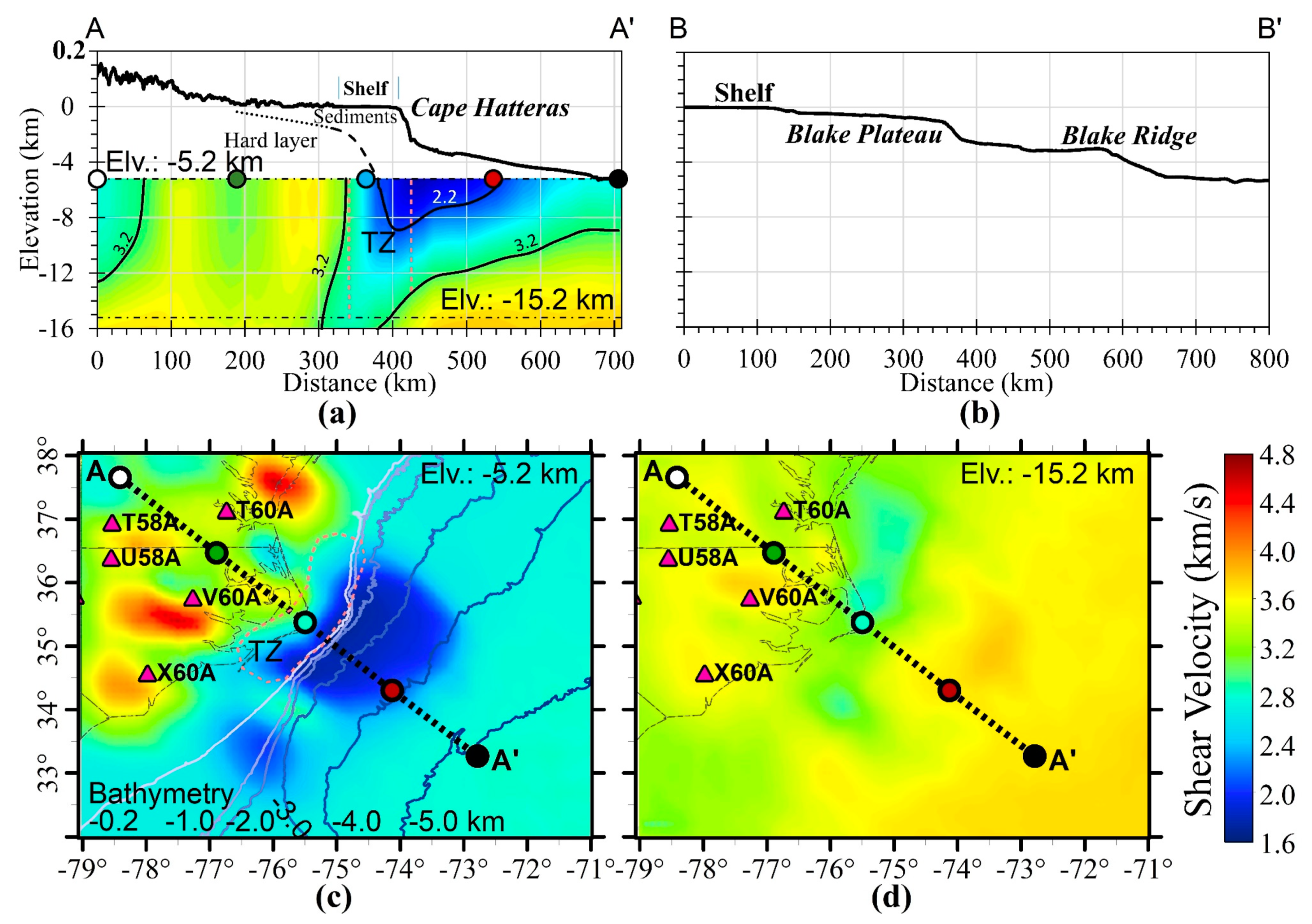
4.2. Types of Continental Margin

In this study, two types of continental margins are identified as exemplified by the transects A-A′ and B-B′ (profile locations are marked in Figure 1) in Figure 9a,b, respectively. Both types have wide (≈100 km) and shallow (<0.2 km) shelves. Along the first type (A-A′), a high (≈2.5 km) and steep slope sharply changes the profile followed by a long gentle slope (continental rise). In the second type (B-B′), the shelf transition into the slope via a wide and gently dipping plateau (Blake Plateau) followed by a shorter (≈1.5 km) and gentler slope (than the first type), then a wide undulating plateau (continental rise) ending with a relatively steep slope.

These differences between the continental margin profiles appear to modify the mechanism of DF microseism generation as suggested by the consistently high spatial densities in the area covering the Blake Ridge and northern Blake Plateau in all three DF bands (Figure 3). A more gradual transition from the shelf and a shorter continental slope are the most prominent features that can support generation of a relatively stable energy level in these areas. Concavity of the continental slope at the edge of the Blake Plateau potentially causes strong reflections resulting in higher DF energy. In contrast, the continental slope at Cape Hatteras has a convex outline that could cause a diffraction pattern, consequently a lower spatial density in this area as shown in the map of the DF1 band in Figure 3. As the DF3 microseisms are generated in the continental shelf, the rough shoreline at Cape Hatteras may be the reason for higher density observed in the DF3 band in Figure 3.

Recent studies also support the hypothesis about the role of the continental slope and show that submarine ridges act similarly to cause reflection of the waves. In [59], by comparing the seasonal variation of DF microseisms and ocean activities, the authors concluded that the DF microseism in the 0.1–0.2 Hz band on the King George Island (on Antarctic Peninsula) originates from a region of Drake Passage instead of the continental shelf around Antarctic Peninsula even though it is several times wider than that around Cape Hatteras. The ocean at Drake Passage is at least 3 km deep and is delimited by the continental slope of Antarctic Peninsula and an underwater ridge roughly normal to the slope. The authors of [33] showed that the excitation locations of both P- and S-wave microseisms observed by a seismometer array in Japan are distributed along the eastern continental slope of Greenland and Reykjanes Ridge extended from Iceland into the deep ocean. An ocean bottom straight blocked by relief features [34,59] promotes formation of ocean wave reflection at the continental slope.

The hypothesis may appear to fail the test based on the observations in [37], who compared the DF spectra (around 0.15 Hz) at three seismometer stations in the coastal region of Oregon and California with the ocean wave climate parameters’ spectra (see their Figure 17). Based on an excellent correlation between DF peak and wave spectra, they concluded that the DF microseism is generated by the wave activities near the shoreline. Significantly different widths of the continental shelves, being much narrower on the western continental margin of North America, and the location of the ocean buoys being on the edge of such a narrow continental shelf (see their Figure 15) can explain the apparent failure. Together with the low frequency (< 0.2 Hz) of their DF peak, it can be argued that the DF microseism observed by [60] was also a result of the reflections from the nearby continental slope as put forward in the proposed hypothesis.

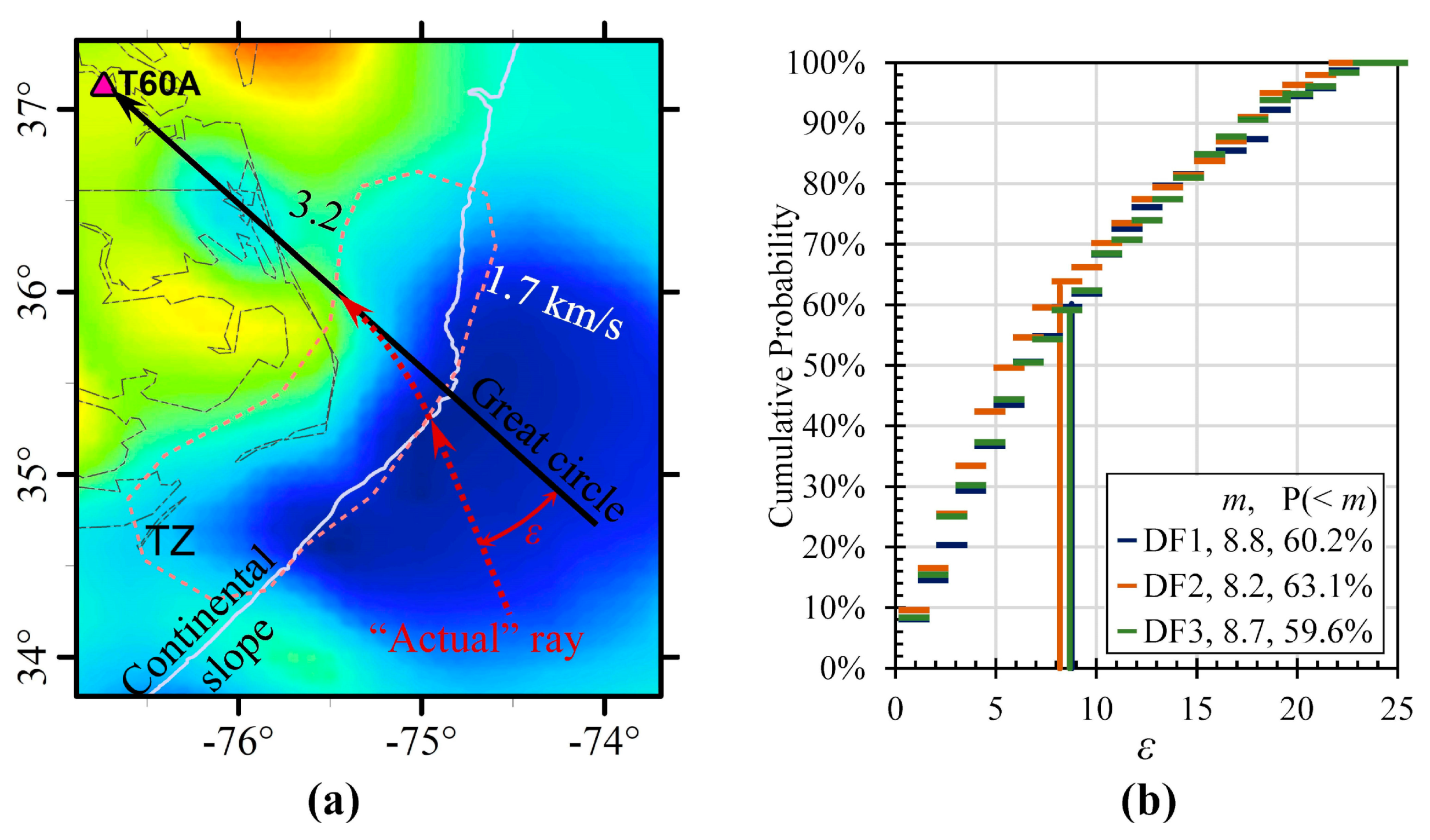
4.3. Rayleigh Wave Refraction

As mentioned in “Data acquisition and processing” section, the Ra and polarization analysis methods to estimate the primary vibration direction are based on an assumption that DF microseisms propagate dominantly as fundamental mode Rayleigh waves. To verify this assumption, Figure 10 was generated to show the probability distributions of the phase differences between the two orthogonal horizontal components (${\mathit{\phi }}_{\mathit{H}\mathit{H}}$) and between the vertical and horizontal components in the primary vibration direction (${\mathit{\phi }}_{\mathit{V}\mathit{H}}$) in the three DF bands. The facts that ${\mathit{\phi }}_{\mathit{H}\mathit{H}}$ is dominant in 0° and ${\mathit{\phi }}_{\mathit{V}\mathit{H}}$ is mainly in 65°–80° and −65°–−80° reveal that the energy is propagating as Rayleigh waves dominantly [61], which coincides well with the observation in [55].

4.3.1. Refraction at the Water–Solid Earth Interface

As explained by [61], when the energy in the DF band is generated from wave–wave interaction in the ocean, it propagates as “pseudo-Rayleigh waves” (pRg) in water column and turns to free surface Rayleigh waves (FSRW) when it reaches solid earth. In the water column, due to phase speed difference, the pRg exists in different forms: dominantly elastic pRg in shallow water with phase speed roughly equal to that of FSRW, and acoustic pRg in deep water with phase speed of about 60% of FSRW. Definitions of shallow and deep waters vary with the wave frequencies. According to the analysis in this study, the energy in LPDF (DF1) band is generated around the continental slope where the water depth is generally smaller than 3000 m (Figure 1), especially on the Blake Plateau (≤ 1000 m) and the edge of the Blake Ridge (≈3000 m). According to Figure 14 in [61], with the increase of frequency from 0.1 to 0.2 Hz, the depth in the water column of elastic pRg dominance decrease from 3000 to 1500 m, under which the elastic pRg transfer to fundamental acoustic pRg. Thus, a phase-speed difference might exist at the water–solid earth interface deeper than 1500 m, i.e., areas except the Blake Plateau, however, the DF energy would still propagate vertically in the water column and transfer to solid earth. Even though there is significant energy loss at the interface, the spherical spreading of the DF energy in the solid earth will not change. Therefore, the phase speed difference on the water–solid earth interface is not likely to affect the determination of the source location by great circle. For high-frequency (0.2–0.5 Hz) DF band, the hypothesis put forward in this manuscript claims that the energy is generated in the continental slope and continental shelf where the water depth is smaller than 200 m. The same figure in [61] shows that the energy in this band should also propagate as elastic pRg and directly transition to FSRW on the continental shelf. As there is no significant phase speed difference between elastic pRg and FSRW, Rayleigh wave refraction at the surface of solid earth is not likely to be significant.

4.3.2. Refraction within the Solid Earth

The Rayleigh wave ray paths are expected to bend also when they travel through the solid earth boundaries with significant impedance contrasts. In order to examine possibility of such boundaries and implications for the validity of the triangulation method, the shear velocity (Vs) structure of the study area is explored as described below.

The cross-section A-A′ presented in Figure 9a shows that under the continental slope there exists a layer of material having Vs less than 2.2 km/s, which is interpreted as sediments in [15]. Our HVSR survey around the eastern foothills of the Appalachian mountain and near the coastal area suggest that the sediment–hard layer interface lies at a depth as depicted by a dotted line in the A-A′ profile in Figure 9a, and that the average Vs of the sediment is about 0.9 km/s [5]. According to [51], the shear velocity contrast at the sediment–hard layer interface should be larger than 2.5 to produce a clear a predominant frequency peak on the HVSR spectrum, therefore, the Vs of the hard layer should be around 2.2 km/s. Therefore, this interface is inferred to connect to the 2.2 km/s contour line (depicted as the dashed line in Figure 9a). Shear velocity gradients are calculated along A-A′ at two different elevations by [15] shear velocity model, and a transitional zone (TZ) of largest shear velocity gradient (where Vs increases from about 1.7 to 3.2 km/s within a horizontal distance of ≈80 km) is identified and outlined as shown in Figure 9a. The TZ at Cape Hatteras (Figure 9c) extend roughly parallel to the continental slope. The absence of notable shear velocity variations at −15.2 km (Figure 9d) suggests that the transitional zone may not extend to this depth.

As explained above, the Rayleigh waves propagating through the solid earth from the deep ocean near the continental slope (DF1 and DF2 bands) or from the continental shelf (DF3 band) to the inland stations are expected to change propagation direction due to gradual and continuous refraction as they pass through TZ. The total refraction angle ε is defined as shown in Figure 11a only for the great circles passing through TZ which represents the worst scenario of changes. The cumulative probability of ε in the three DF bands is given in Figure 11b. The weighted average (m) of ε in DF1, DF2, and DF3 bands are calculated to be 8.8°, 8.2°, and 8.7°, respectively, and the probabilities of ε values less than these corresponding weighted averages (P < m) are 60.2%, 63.1%, and 59.6%.

Another examination of the Rayleigh wave refraction from sediments to bedrock is carried out by tracking hurricane “Sandy” in Atlantic Ocean on 27 October 2012 using 8 h ambient noise recorded on the bedrock in Tishomingo, Mississippi. The DF peak is found at the central frequency of 0.18 Hz with very high energy. The primary vibration direction at this central frequency is calculated by both Ra and Polarization analysis methods and projected as great circles which point to the locations of hurricane “Sandy” successfully (see Figure S4 in the Supplementary Materials to this article). Thus, the great circles can be considered as valid projections to the source areas of the DF energy.

4.4. Rayleigh Wave Refraction

According to the hypothesis and the discussion above, the DF microseisms in the LPDF (DF1) band is generated in the deep ocean close to the continental slope and propagate to stations on land. Depending on the location of the stations, the propagation paths are different, i.e., through sediments and bedrock to stations on inland bedrock, and through sediments on coastal stations on sediments, resulting in different attenuations and energy levels at stations. This difference is observed in this study. In Figure 3, the PSD levels in the DF1 band increase from coast (sediments) to inland (Appalachian Mountain) while the distance to source (ocean) increases. The possible explanation is that the attenuation due to spherical spreading is less effective than energy absorption in sediments. A similar trend is observed by [55] in the same study area. In the DF2 band, the PSD levels at coastal stations are slightly larger than or equal to those at inland stations, which might because the attenuation due to spherical spreading and absorption in sediments are equally effective. In the DF3 band, the PSD levels at coastal stations are obviously larger than those at inland stations, as the attenuation is dominantly spherical spreading and absorption effect is equally effective, which reveals that the DF microseisms in this band are generated in the continental shelf and propagate mainly in sediments.

5. Conclusions

This study explored the role and significance of the continental slope in the interactions between the ocean waves and the continental margin as well as the resulting double-frequency (DF) microseisms recorded in ENAM. The primary vibration direction analysis of the ambient noise recordings in the study area shows that these DF microseisms originated in areas of the North Atlantic Ocean, which are generally aligned in the SE direction with the recording stations. The great circles corresponding to these primary vibration directions for different DF peaks intersect at a number of locations enabling delineation of source areas along the continental slope. Correlation analysis between DF microseisms and ocean wave climate by considering the correspondence in their frequency composition and variation in energy levels shows that the DF microseisms in DF1 (0.1–0.2 Hz), DF2 (0.2–0.3 Hz), and DF3 (0.3–0.4 Hz) bands correlate well with the ocean wave activities in the continental slope on the deep ocean side, and in the continental slope on both the deep ocean and shelf sides, and in the continental slope on the shelf side, respectively. These analyses lead to a hypothesis on the frequency dependent interactions of ocean waves with the continental margin and the origination of DF microseisms. The steep continental slope is a key submarine topographic feature which behaves as an obstacle causing reflections of the incoming low frequency (≤ 0.15 Hz) ocean waves and formation of standing waves to generate low frequency (≤ 0.3 Hz) DF microseisms. While the high frequency (≥ 0.15 Hz) ocean waves are reflected at the shallow portion of the continental shelf to excite high frequency (≥ 0.3 Hz) DF microseisms. This hypothesis is also supported by the observations that (1) the great circles corresponding to the primary vibration directions of DF microseisms are mostly normal to the strike of the continental slope; and (2) the ocean wave energy in the continental slope or the nearby deep ocean are higher than in the distant deep ocean and the continental shelf. Additional systematic observations at different parts of the globe will help to determine validity and limits of the proposed hypothesis under all possible climatic and bathymetric conditions.

Understanding the generation mechanisms and locating the source regions of the DF microseisms would improve the reliability of estimating the amplification factor based on ambient noise because the amplification process could be understood by bridging the variations of the input energy levels at the sources and the energy at the site. In addition, DF microseisms recordings at the coastal areas suggests that the sources are not homogeneously distributed. However, surface wave tomography could be carried out only if the noise sources are homogenously distributed. Therefore, locating the source regions could improve the current method of tomography or initiate a new method using non-homogenous ambient noise.

With the frequency dependent interactions between the ocean waves and the continental margin determined, one could further analyze the possible mass wasting on the continental margin caused by the ocean wave energy input and transmission while ocean waves interact with the continental margin.

References

1. Nakamura, Y. A method for dynamic characteristics estimation of subsurface using microtremor on the ground surface. QR of RTRI 1989, 30, 25–33. [Google Scholar]
2. Bodin, P.; Horton, S. Broadband microtremor observation of basin resonance in the Mississippi embayment, Central US. Geophys. Res. Lett. 1999, 26, 903–906. [Google Scholar] [CrossRef]
3. Bodin, P.; Smith, K.; Horton, S.; Hwang, H. Microtremor observations of deep sediment resonance in metropolitan Memphis, Tennessee. Eng. Geol. 2001, 62, 159–168. [Google Scholar] [CrossRef]
4. Bard, P.-Y.; SESAME-team. Guideline for the Implementation of the H/V Spectral Ratio Technique on Ambient Vibrations-Measurements, Processing and Interpretations; SESAME European Research Project EVG1-CT-2000-00026, D23.12. 2005. Available online: http://sesame-fp5.obs.ujf-grenoble.fr/index.htm (accessed on 19 February 2020).
5. Guo, Z.; Aydin, A.; Kuszmaul, J. Microtremor recording in northern Mississippi. Eng. Geol. 2014, 179, 146–157. [Google Scholar] [CrossRef]
6. Lobkis, O.I.; Weaver, R.L. On the emergence of the Green’s function in the correlations of a diffuse field. J. Acoust. Soc. Am. 2001, 110, 3011–3017. [Google Scholar] [CrossRef] [Green Version]
7. Snieder, R. Extracting the Green’s function from the correlation of coda waves: A derivation based on stationary phase. Phys. Rev. E 2001, 69, 046610. [Google Scholar] [CrossRef] [Green Version]
8. Shapiro, N.M.; Campillo, M. Emergence of broadband Rayleigh waves from correlations of the ambient seismic noise. Geophys. Res. Lett. 2004, 31, L07614. [Google Scholar] [CrossRef] [Green Version]
9. Shapiro, N.M.; Campillo, M.; Stehly, L.; Ritzwoller, M.H. High resolution surface wave tomography from ambient seismic noise. Science 2005, 307, 1615–1618. [Google Scholar] [CrossRef] [Green Version]
10. Sabra, K.G.; Gerstoft, P.; Roux, P.; Kuperman, W.A.; Fehler, M.C. Extracting time-domain Green’s function estimates from ambient seismic noise. Geophys. Res. Lett. 2005, 32, L03310. [Google Scholar] [CrossRef]
11. Sabra, K.G.; Gerstoft, P.; Roux, P.; Kuperman, W.A.; Fehler, M.C. Surface wave tomography from microseisms in Southern California. Geophys. Res. Lett. 2005, 32, L14311. [Google Scholar] [CrossRef] [Green Version]
12. Yang, Y.; Ritzwoller, M. Characteristics of ambient seismic noise as a source for surface wave tomography. Geochem. Geophys. Geosyst. 2008, 9, Q02008. [Google Scholar] [CrossRef] [Green Version]
13. Yang, Y.; Ritzwoller, M.; Levshin, A.; Shapiro, N. Ambient noise Rayleigh wave tomography across Europe. Geophys. J. Int. 2007, 168, 259–274. [Google Scholar] [CrossRef] [Green Version]
14. Stephenson, W.J.; Hartzell, S.; Frankel, A.D.; Asten, M.; Carver, D.L.; Kim, W.Y. Site characterization for urban seismic hazards in lower Manhattan, New York City, from microtremor array analysis. Geophys. Res. Lett. 2009, 36, L03301. [Google Scholar] [CrossRef]
15. Lynner, C.; Porritt, R.W. Crustal structure across the eastern North American margin from ambient noise tomography. Geophys. Res. Lett. 2017, 44, 6651–6657. [Google Scholar] [CrossRef] [Green Version]
16. Guo, Z.; Aydin, A. A modified HVSR method to evaluate site effect in Northern Mississippi considering ocean wave climate. Eng. Geol. 2016, 200, 104–113. [Google Scholar] [CrossRef]
17. Stehly, L.; Campillo, M.; Shapiro, N.M. A study of the seismic noise from its long-range correlation properties. J. Geophys. Res. 2006, 111, B10306. [Google Scholar] [CrossRef]
18. Shapiro, N.M.; Ritzwoller, M.H.; Bensen, G.D. Source location of the 26 sec microseism from cross-correlation of ambient seismic noise. Geophys. Res. Lett. 2006, 33, L18310. [Google Scholar] [CrossRef] [Green Version]
19. Tsai, V.C. On establishing the accuracy of noise tomography travel-time measurements in a realistic medium. Geophys. J. Int. 2009, 178, 1555–1564. [Google Scholar] [CrossRef] [Green Version]
20. Zeng, X.; Ni, S. A persistent localized microseismic source near the Kyushu Island, Japan. Geophys. Res. Lett. 2010, 37, L24307. [Google Scholar] [CrossRef]
21. Ermert, L.; Villaseñor, A.; Fichtner, A. Cross-correlation imaging of ambient noise sources. Geophys. J. Int. 2016, 204, 347–364. [Google Scholar] [CrossRef]
22. Guo, Z.; Xue, M.; Aydin, A.; Ma, Z. Exploring source regions of single- and double-frequency microseisms recorded in eastern North American margin (ENAM) by cross-correlation. Geophys. J. Int. 2020, 220, 1352–1367. [Google Scholar] [CrossRef]
23. Longuet-Higgins, M.S. A theory for the generation of microseisms. Philos. Trans. R. Soc. Lond. 1950, 243, 1–35. [Google Scholar]
24. Hasselmann, K. A statistical analysis of the generation of microseisms. Rev. Geophys. Space Phys. 1963, 1, 177–210. [Google Scholar] [CrossRef]
25. Bromirski, P.D.; Duennebier, F.K.; Stephen, R.A. Mid-ocean microseisms. Geochem. Geophys. Geosyst. 2005, 6, Q04009. [Google Scholar] [CrossRef]
26. Essen, H.-H.; Krüger, F.; Dahm, T.; Grevemeyer, I. On the generation of secondary microseisms observed in northern and central Europe. J. Geophys. Res. 2003, 108, 2506. [Google Scholar] [CrossRef]
27. Obrebski, M.J.; Ardhuin, F.; Stutzmann, E.; Schimmel, M. How moderate sea states can generate loud seismic noise in the deep ocean. Geophys. Res. Lett. 2012, 39, L11601. [Google Scholar] [CrossRef] [Green Version]
28. Rhie, J.; Romanowicz, B. A study of the relation between ocean storms and the Earth’s hum. Geochem. Geophys. Geosyst. 2006, 7, Q10004. [Google Scholar] [CrossRef]
29. Schimmel, M.; Stutzmann, E.; Ardhuin, F.; Gallart, J. Polarized Earth’s ambient microseismic noise. Geochem. Geophys. Geosyst. 2011, 12, Q07014. [Google Scholar] [CrossRef] [Green Version]
30. Stephen, R.A.; Spiess, F.N.; Collins, J.A.; Hildebrand, J.A.; Orcutt, J.A.; Peal, K.R.; Vernon, F.L.; Wooding, F.B. Ocean seismic network pilot experiment. Geochem. Geophys. Geosyst. 2003, 4, 1092. [Google Scholar] [CrossRef]
31. Webb, S.C. Broadband seismology and noise under the ocean. Rev. Geophys. 1998, 36, 105–142. [Google Scholar]
32. Traer, J.; Gerstoft, P.; Bromirski, P.D.; Shearer, P.M. Microseisms and hum from ocean surface gravity waves. J. Geophys. Res. 2012, 117, B11307. [Google Scholar] [CrossRef] [Green Version]
33. Nishida, K.; Takagi, R. Teleseismic S wave microseism. Science 2016, 353, 919–921. [Google Scholar] [CrossRef] [PubMed]
34. Gerstoft, P.; Bromirski, P. “Weather bomb” induced seismic signals. Science 2016, 353, 869–870. [Google Scholar] [CrossRef] [PubMed]
35. Elgar, S.; Herbers, T.H.C.; Guza, R.T. Reflection of ocean surface gravity waves from a natural beach. J. Phys. Oceanogr. 1994, 24, 1503–1511. [Google Scholar] [CrossRef]
36. Ardhuin, F.; Stutzmann, E.; Schimmel, M.; Mangeney, A. Ocean wave sources of seismic noise. J. Geophys. Res. 2011, 116, C09004. [Google Scholar] [CrossRef]
37. Bromirski, P.D.; Duennebier, F.K. The near-coastal microseism spectrum: Spatial and temporal wave climate relationships. J. Geophys. Res. 2002, 107, B8. [Google Scholar] [CrossRef] [Green Version]
38. Ardhuin, F.; Roland, A. Coastal wave reflection, directional spread, and seismoacoustic noise sources. J. Geophys. Res. 2012, 117, C00J20. [Google Scholar] [CrossRef] [Green Version]
39. Gualtieri, L.; Stutzmann, E.; Capdeville, F.; Farra, V.; Mangeney, A.; Morelli, A. On the shaping factors of the secondary microseismic wavefield. J. Geophys. Res. 2015, 120. [Google Scholar] [CrossRef] [Green Version]
40. Sutton, G.; Barstow, N. Ocean bottom microseisms from a distant supertyphoon. Geophys. Res. Lett. 1996, 23, 499–502. [Google Scholar] [CrossRef]
41. Bromirski, P.D.; Flick, R.E.; Graham, N. Ocean wave height determined from inland seismometer data: Implications for investigating wave climate change in the NE Pacific. J. Geophys. Res. 1999, 104, 20753–20766. [Google Scholar] [CrossRef]
42. Dorman, L.M.; Schreiner, A.E.; Bibee, L.D.; Hildebrand, J.A. Deep-Water Seafloor Array Observations of Seismo-Acoustic Noise in the Eastern Pacific and Comparisons with Wind and Swell, in Natural Physical Source of Underwater Sound; Kerman, B., Ed.; Springer: New York, NY, USA, 1993; pp. 165–174. [Google Scholar]
43. Ebeling, C.W. Chapter One–inferring ocean storm characteristics from ambient seismic noise: A historical perspective. Adv. Geophys. 2012, 53, 1–33. [Google Scholar]
44. Guo, Z.; Aydin, A. Double-frequency microseisms in ambient noise recorded in Mississippi. Bull. Seismol. Soc. Am. 2015, 105, 1691–1710. [Google Scholar] [CrossRef]
45. Park, J.; Verono III, F.L.; Lindberg, C.R. Frequency dependent polarization analysis of high-frequency seismograms. J. Geophys. Res. 1987, 92, 12664–12674. [Google Scholar] [CrossRef]
46. Cessaro, R.K. Sources of primary and secondary microseisms. Bull. Seismol. Soc. Am. 1994, 84, 142–148. [Google Scholar]
47. Friedrich, A.; Krüger, F.; Klinge, K. Ocean-generated microseismic noise located with the Gräfenberg array. J. Seismol. 1998, 2, 47–64. [Google Scholar] [CrossRef]
48. Nishida, K.; Kawakatsu, H.; Fukao, Y.; Obara, K. Background Love and Rayleigh waves simultaneously generated at the Pacific Ocean floors. Geophys. Res. Lett. 2008, 35, L16307. [Google Scholar] [CrossRef] [Green Version]
49. Paskevich, V. Srtm30plus-na_pctshade.tif—SRTM30PLUS color-encoded shaded relief image of North America (approximately 1km)—GeoTIFF image: Open-File Report 2005-1001, U.S. Geological Survey, Coastal and Marine Geology Program; Woods Hole Science Center: Woods Hole, MA, USA, 2005; 30p. [Google Scholar]
50. Bard, P.-Y. Microtremor measurements: A tool for site effect estimation? In Proceedings of the 2nd International Symposium on the Effects of Surface Geology on Seismic Motion, Yokohama, Japan, 1–3 December 1998; pp. 1251–1279. [Google Scholar]
51. Konno, K.; Ohmachi, T. Ground-motion characteristics estimated from spectral ratio between horizontal and vertical components of microtremor. Bull. Seismol. Soc. Am. 1998, 88, 28–241. [Google Scholar]
52. McNamara, D.E.; Buland, R.P. Ambient noise levels in the continental United States. Bull. Seismol. Soc. Am. 2004, 94, 1517–1527. [Google Scholar] [CrossRef]
53. Bendat, J.S.; Piersol, A.G. Random Data: Analysis and Measurement Procedures; Wiley-Interscience: New York, NY, USA, 1971. [Google Scholar]
54. Havskov, J.; Ottemoller, L. Routine Data Processing in Earthquake Seismology; Springer: New York, NY, USA, 2010; 347p. [Google Scholar]
55. Koper, K.D.; Burlacu, R. The fine structure of double-frequency microseisms recorded by seismometers in North America. J. Geophys. Res. 2015, 120. [Google Scholar] [CrossRef]
56. Babcock, J.M.; Kirkendall, B.A.; Orcutt, J.A. Relationship between ocean bottom noise and the environment. Bull. Seismol. Soc. Am. 1994, 84, 1991–2007. [Google Scholar]
57. Kibblewhite, A.C.; Ewans, K.C. Wave-wave interactions, microseism, and infrasonic ambient noise in the ocean. J. Acoust. Soc. Am. 1985, 78, 981–994. [Google Scholar] [CrossRef]
58. Schreiner, A.E.; Dorman, L.M. Coherence lengths of seafloor noise: Effect of ocean bottom structure. J. Acoust. Soc. Am. 1990, 88, 1503–1514. [Google Scholar] [CrossRef]
59. Lee, W.S.; Sheen, D.H.; Yun, S.; Seo, K.W. The origin of double-frequency microseism and its seasonal variability at King Sejong Station, Antarctica. Bull. Seismol. Soc. Am. 2011, 106, 1446–1451. [Google Scholar] [CrossRef]
60. Koper, K.D.; Hawley, V.L. Frequency dependent polarization analysis of ambient seismic noise recorded at a broadband seismometer in the central United States. Earthq. Sci. 2010, 23, 439–447. [Google Scholar] [CrossRef] [Green Version]
61. Bromirski, P.D.; Stephen, R.A.; Gerstoft, P. Are deep-ocean-generated surface-wave microseisms observed on land? J. Geophys. Res. 2013, 118, 3610–3629. [Google Scholar] [CrossRef] [Green Version]
Figure 1. Study area and locations of transportable array (TA) stations (triangles) and buoys (yellow circles) of National Oceanic and Atmospheric Administration, recordings of which are analyzed in this study. The table lists the original numbers and a simplified numbering scheme of the ocean buoys grouped according to their four distinct locations: deep ocean (DO), the continental slope-deep ocean side (SlDO), the continental slope-shelf side (SlSh), and the continental shelf (Sh). The color-encoded relief base map is from [49]. The black lines A-A′ and B-B′ are the transects presented in Figure 9a,b. The white box indicates the area where the underground shear velocity model (Figure 9c,d) was computed based on [15].
Jmse 08 00134 g001
Figure 2. (a) Power spectral density (PSD) plots in time-frequency domain of the vertical components at the selected stations. The dashed lines at 0.2 and 0.3 Hz mark the boundaries of the three frequencies ranges. Three relatively strong double-frequency (DF) microseism events are identified and labeled as I, II, and III. (b) Polar plots of average R a ( φ ) values (blue) combined with rose diagrams of back azimuths (calculated by the polarization analysis) (purple) at the three DF bands at the selected stations in the whole recording period. On each plot, the text labels refer to the recording station (e.g., N61A), probability of back azimuth (in purple, e.g., 10%) and the scale of the solid outer circle in multiples of the R a ( φ ) value (in blue, e.g., Ra = 2). The same plots for the remaining stations are shown in Figure S1 in the Supplementary Materials.
Jmse 08 00134 g002
Figure 3. The normalized spatial density (color gradient maps) of the great circles corresponding to the daily primary vibration directions ( φ m 1 ) and the vertical PSDs averaged for the entire recording period (scaled circles) in the three DF bands. The yellow lines contour the density of 0.5. The rose diagram shows the probability distribution of all φ m 1 s.
Jmse 08 00134 g003
Figure 4. (a,c,e) Daily WAVEWATCH III hindcasts of ocean wave spectra (E(F/2) in log10 (m2/Hz)) in Northern Atlantic Ocean (color gradient maps), PSD levels (small circles with scaled sizes), and primary vibration directions (segments of great circles) at all stations corresponding to the three events (I, II, and III) identified in Figure 2. The purple circles/ellipses delimit the intersections of the great circles; (b,d,f) Time history of average PSDs in three frequency bands. In each plot, the curves are stacked by the latitudes of the stations and the relief of each curve shows the change of PSD level. The starting time of the three events are picked and connected to form the red lines, the arrows of which show the impact sequence.
Jmse 08 00134 g004
Figure 5. Average Pearson correlation coefficients (CC) between the PSDs in the three DF bands and the ocean wave heights in four groups of ocean buoys.
Jmse 08 00134 g005
Figure 6. Difference of the ocean wave energy (E(F/2) in log10(m2/Hz)) and PSD levels between day 329 and 331 (Figure 4c,e, respectively).
Jmse 08 00134 g006
Figure 7. A sketch describing how constructive interactions of ocean waves and their reflections from a barrier (the continental slope or the shoreline) can result in different energies when the angle of incidence is (a) large and (b) 0°. Note a given station receives the strongest signals along the shortest path A.
Jmse 08 00134 g007
Figure 8. (a) Defining the angle δ (<90°) between a great circle and the continental slope’s strike. (b) Histogram of the angles δ s in the three DF bands.
Jmse 08 00134 g008
Figure 9. Topographic profiles of the continental margin along (a) A-A′ and (b) B-B′ (marked in Figure 1) based on General Bathymetric Chart of the Oceans (GEBCO, 2014). The shear velocity profile and contours in (a) are reproduced on [15]. The geophysical interface between sediments and bedrock is estimated (black dotted line) by horizontal-to-vertical spectral ratio (HVSR) method and was extended seaward by inference (black dashed line) to connect with the 2.2 km/s shear velocity contour. A transitional zone (TZ) with the largest shear velocity gradient is identified and outlined by the two pink dashed lines in (a). The shear velocity models inside the white box outlined in Figure 1 are generated for elevations (Elv.) of −5.2 km (c) and −15.2 km (d) based on [15].
Jmse 08 00134 g009
Figure 10. Probability distribution of the phase difference between (a) the two horizontal components ( φ H H ) and (b) the vertical and horizontal component in the primary vibration direction ( φ V H ).
Jmse 08 00134 g010
Figure 11. (a) Defining angle ε to measure total refraction of Rayleigh wave ray passing through the transitional zone (TZ in Figure 9a,c) taking a ray path to station T60A as an example. The black solid and red dotted lines are the great circle projected in this study and “actual” ray path of Rayleigh wave, respectively. (b) Cumulative probability of ε for waves in the three DF bands propagating through TZ.
Jmse 08 00134 g011