Article

Numerical Investigation into Freak Wave Effects on Deepwater Pipeline Installation

1
College of Civil Engineering, Fuzhou University, Fuzhou 350116, China
2
Institute of Structural Engineering, Zhejiang University, Hangzhou 310058, China
*
Author to whom correspondence should be addressed.
J. Mar. Sci. Eng. 2020, 8(2), 119; https://doi.org/10.3390/jmse8020119
Submission received: 18 January 2020 / Revised: 31 January 2020 / Accepted: 3 February 2020 / Published: 14 February 2020

Abstract

:
Freak waves are an extreme marine environment factor in offshore structure design and become a potential risk, particularly for laying oil-gas pipelines in deep waters. The objective of this study was to reveal the freak wave effects on dynamic behaviors of offshore pipelines for deepwater installation. Thus, a dedicated finite element model (FEM) for deepwater pipeline installation by the S-lay method was developed with special consideration of freak waves. The FEM also took pipelay vessel motions, pipe–stinger roller interactions, and the cyclic contacts between the pipeline and seabed soil into account. Real vessel and stinger data from an actual engineering project in the South China Sea were collected to obtain an accurate simulation. Moreover, an effective superposition approach of combined transient wave trains and random wave trains was introduced, and various types of freak wave trains were simulated. Extensive numerical analyses of a 12 inch gas pipeline being installed into a water depth of 1500 m were implemented under various freak wave conditions. The noticeable influences of freak waves on the pipeline and seabed responses were identified, which provides significant awareness of offshore pipelines for deepwater installation design and field operation monitoring.

1. Introduction

Freak waves occur unexpectedly far out at sea with remarkably large wave heights and are deemed to be an extreme marine environment condition. The irregular distribution of freak wave heights does not comply with the basic law of Rayleigh distribution for normal ocean waves, especially in deep waters. The unique feature of freak waves makes it difficult for marine structural engineers to sufficiently consider the huge wave loads in the design stage. In the past, plenty of tremendous accidents, including shipwrecks and massive destruction of offshore structures, have been caused by the great impact of freak waves [1,2]. These accidents have produced a striking warning on the potential risk of freak waves for lay barge and offshore structures and have attracted wide attention on the investigation into freak-wave-induced structural responses.
The offshore pipeline is a representative type of marine structure that is widely utilized for crude oil and natural gas transportation from subsea well sites to surface processing facilities. In recent years, the great demand for energy resources has facilitated the expansion of oil-gas exploitation into deepwater areas. The S-lay approach is one of most common methods of deepwater pipeline installation to the sea floor owing to its excellent adaptability and workability [3]. In this pipelay technique, numerous section pipes with designed lengths are welded and inspected on the operating lines of the vessel. The qualified pipeline is drawn by the tensioners and slides over the stinger to arrive at the seabed. The overall pipeline is characterized as an S-shaped curve and divided into two regions, as displayed in Figure 1. The upper curved section of the pipeline from the tensioner to the lift-off point (LOP) is denoted as the overbend, and the suspended section from the LOP to the seabed is known as the sagbend. The whole process of laying the pipeline generally takes months or even longer periods, and is more likely to encounter the occurrence of freak waves. Therefore, to assess the influences of freak waves on the dynamic behaviors of S-laying pipelines in deep waters is highly significant for the purpose of pipelay design and operation safety.
A reasonable wave generation method is necessary to simulate freak waves and explore their impact on marine structures. A numerical technique is extensively employed due to its convenient simulation and good repeatability. Davis and Zarnick [4] initially proposed a wave focusing method to simulate freak waves by controlling the focalized time and space. Subsequently, Baldock et al. [5] applied the technique to accumulate numerous water waves and produce a huge transient wave group. Fochesato et al. [6] superposed wave trains of different directions to generate three-dimensional (3D) freak waves. Zhao et al. [7,8] presented four focusing models to generate the freak wave trains and numerically simulated the wave effect on a floating structure. Liu et al. [9] developed a modified phase modulation approach to focus wave trains with the specified phase and obtained the precise wave spectrum that coincided well with the target results. Hu et al. [10] employed a probability-based superposition method to calculate the generation probability of a freak wave. Recently, Tang et al. [11] improved the phase modulation model to generate a freak wave and investigated its effect on the dynamic responses of the Floating Production Storage and Offloading (FPSO) and Single Point Mooring (SPM) system. Pan et al. [12] conducted extensive tests to observe the great differences in cylinder motion responses under irregular waves and freak waves and obtained the important influencing factors. The wave focusing and superposition techniques were demonstrated to effectively generate freak wave trains, which provided a prior simulation of the wave impact on pipeline installation in deepwater areas.
Under the excitation of surface waves and vessel motions, the laying pipelines usually exhibit sophisticated non-linear, dynamic responses. The complicated S-lay problems mainly result from large pipeline deflections, pipe material plasticity, hydrodynamic loads, and boundary interactions. These non-linear features could cause some difficulties for analytical approaches and experimental tests to obtain accurate and comprehensive simulations. As a consequence, numerical techniques are preferred for modeling systematical behaviors of offshore pipelines in the S-lay process [13,14,15]. Gong et al. [16] and Gong and Xu [17] developed a full FEM on the basis of OrcaFlex to simulate the structural behaviors of pipeline installation and explored the influence of normal sea states on the pipeline responses. Ivić et al. [18,19] established a pipeline laying model by the use of non-linear elastic beam elements to analyze the static behaviors of the S-laying pipe and formulated a specialized optimization method for the pipeline laying operation. Xie et al. [20] investigated the dynamic loading history of laying pipelines in light of a test-verified FEM and confirmed obvious pipeline plastic deformations resulting from the S-lay operation. Cabrera-Miranda and Paik [21] quantified the probabilistic distribution of loads on a marine riser and observed the highly random characteristic of the loads to aid in the determination of nominal design values. Wang et al. [22] pointed out the probable underestimation of pipeline dynamic behaviors for practical engineering and built a real-time installation monitoring system to predict on-site pipeline responses. Recently, Liang et al. [23,24] presented a refined FEM to take account of the complex surface contact behaviors of overbend pipes and reproduced the pipe laying process of a deep S-lay case in the laboratory. Kim and Kim [25] employed the FEM-based linear beam element to present an efficient, linearized, dynamic analysis approach for pipeline installation design. The aforementioned studies usually adopted normal random waves as the input ocean conditions to calculate the dynamic responses of laying pipelines. The neglect of the freak wave effect could result in the inadequacy of pipeline installation design for field operation safety.
The objective of this study was to thoroughly investigate the freak wave effects on the dynamic responses of offshore pipelines during deepwater S-lay installation. A new extended FEM with particular consideration of freak waves was developed on the basis of our previous model [16] for S-lay pipelines. This model took the induced vessel motions, pipe–stinger roller contacts, and pipe–seabed soil interactions into account. The real vessel, stinger roller, and seabed soil data from an actual engineering project in South China Sea were collected to obtain an accurate simulation. Furthermore, an effective superposition technique was employed to generate freak waves by combining transient wave trains and random wave trains. The insertion of various freak wave trains into the S-lay FEM was then implemented to carry out a large number of numerical analyses of a 12 inch gas pipeline being installed into a 1500 m water depth. Finally, the influences of the freak wave energy ratio coefficient, focusing location, phase range, and peak value were sufficiently assessed on the pipeline and seabed responses. The dynamic amplification factors (DAFs) of the axial tension, bending moment, von Mises stress, longitudinal strain, pipeline embedment, and seabed resistance are discussed in detail in relation to pipeline installation design and field operation safety.

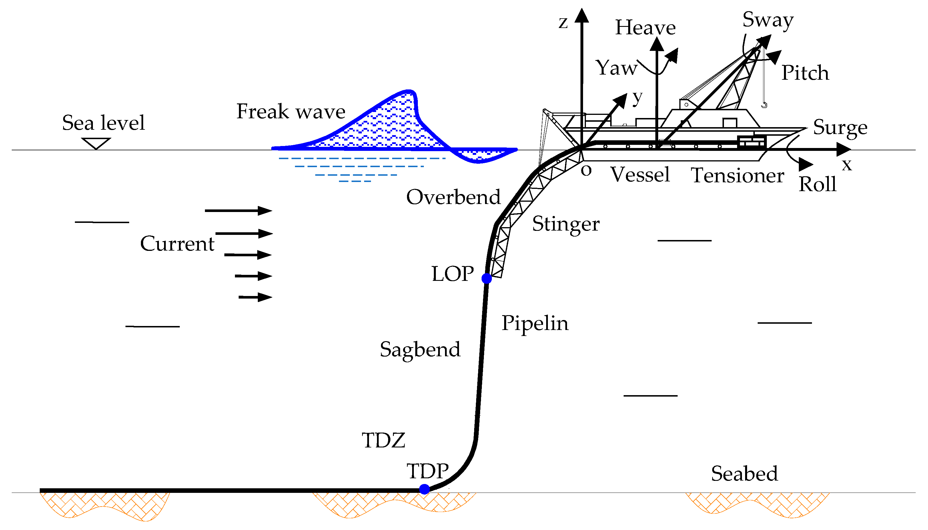
2. Deepwater Pipeline Installation Simulation
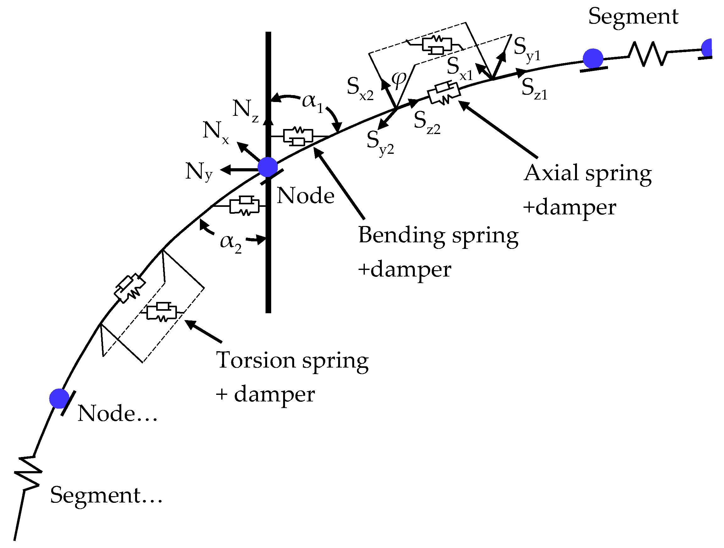
A reasonable FEM for S-lay system was presented by Gong et al. [16] to explore the random wave effects on the dynamic behaviors of deepwater pipeline installation. This model, developed within the framework of OrcaFlex [26], was validated with acceptable accuracy and effective applicability by an actual engineering case of S-laying pipelines. In this study, a new extension of the FEM was implemented to consider the freak waves with wave-induced pipeline behaviors, pipe–stinger roller contacts, pipe–seabed soil interaction, and pipelay vessel motions, as displayed in Figure 1. The following section presents a concise description of the main features of the deepwater pipeline installation model by the S-lay technique.

2.1. Pipeline Model

In the FEM of the S-lay system, the entire pipeline, from the tensioner to the sea floor, was discretized into a sequence of mass nodes connected together by massless line segments, as displayed in Figure 2. The local xyz-frames of references for the node and line segment were established, and the mechanical properties of the pipe weight, buoyancy, drag force, and so on for each half-segment were concentrated on its adjacent node. At either side of the node, two rotational springs and dampers were employed to model the bending stiffness and damping of the line segment. At the center of the line segment, an axial spring with a damper was utilized to represent its axial stiffness and damping, and a torsional spring with a damper was applied to characterize its torsional stiffness and damping. For the detailed calculation derivation of the tension force, bending moment, and torque moment, one can refer to the literature [16], and their expressions are given by
T e = T w ( ε ) + ( 1 - 2 ν ) ( P o A o P i A i ) + E A nom ξ ( d L / d t ) / L 0
M 2 = M b ( κ 2 ) + ς ( d κ 2 / d t )
T t = T or ( ϕ / L 0 ) + ζ ( d ϕ / d t )
where Te and Tw are the effective tension and wall tension relating to the axial strain; Pi and Po are the internal pressure and external pressure; Ai and Ao are the internal and external cross-section areas; ν is the Poisson’s ratio; EAnom is the nominal axial stiffness defined at zero strain; L is the instantaneous length of the line segment; L0 is the unstretched length of the line segment; Mb is the bending moment relating to the curvature κ2; Tor is the torque moment relating to the twist angle φ; and the damping coefficients ξ, ς and ζ separately represent axial, bending, and torsional effects of structural damping.
The oil-gas pipelines installed in deep waters comprise carbon–manganese steel with a distinct yield point and some plastic deformation capability. The pipeline material features were simulated by the J2 flow theory of plasticity performance with isotropic strain hardening. The Ramberg–Osgood model [27] was applied to represent the non-linear stress and strain relationship of the adoptive X65 line pipe, which could be expressed as
ε ( σ ) = σ / E + B ( σ / σ y ) n
where σ y is the effective yield stress, E is the elastic modulus, and B and n are the coefficient and the power exponent of the constitutive model.

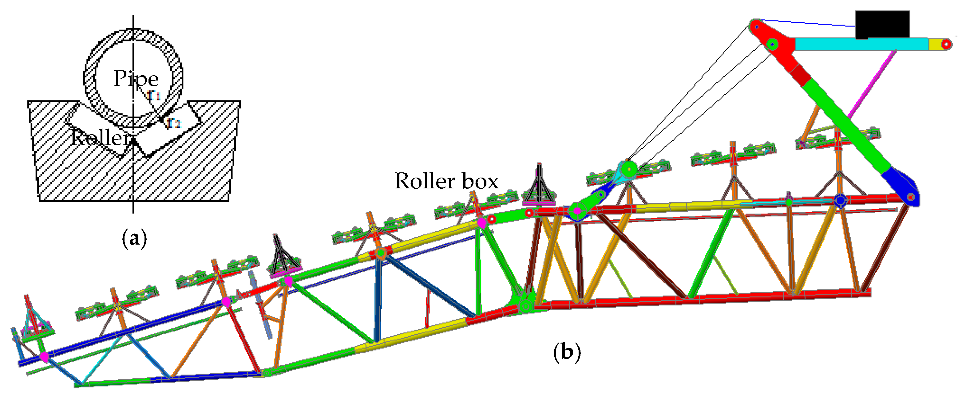
2.2. Pipe–Stinger Roller Interaction

In the overbend, the sections of the pipeline were continuously supported by 10 roller boxes that were regularly spaced and settled on the articulated stinger, which was 75 m in length, as illustrated in Figure 3. The stinger with three sections of truss structure was collected from the actual design for the Hai Yang Shi You (HYSY) 201 pipelay vessel [28]. A group of pipe segments was employed to simulate the stinger’s geometrical and mechanical properties. The clashing contacts between the pipeline and stinger rollers would vary with the vessel motions. Before the calculation of pipe–stinger roller interactions, an inspection had to be implemented to confirm whether the pipeline was in contact with the roller. If a mutual interaction was identified, the contact force was calculated and applied to the pipe and the roller, which was given by
F r = [ 1 / ( 1 / k 1 + 1 / k 2 ) ] × [ d ( r 1 + r 2 ) ]
where k1 and k2 are the contact stiffness of the pipe and the roller, d is the shortest separation distance of the center lines between them, and r1 and r2 are the corresponding radii.

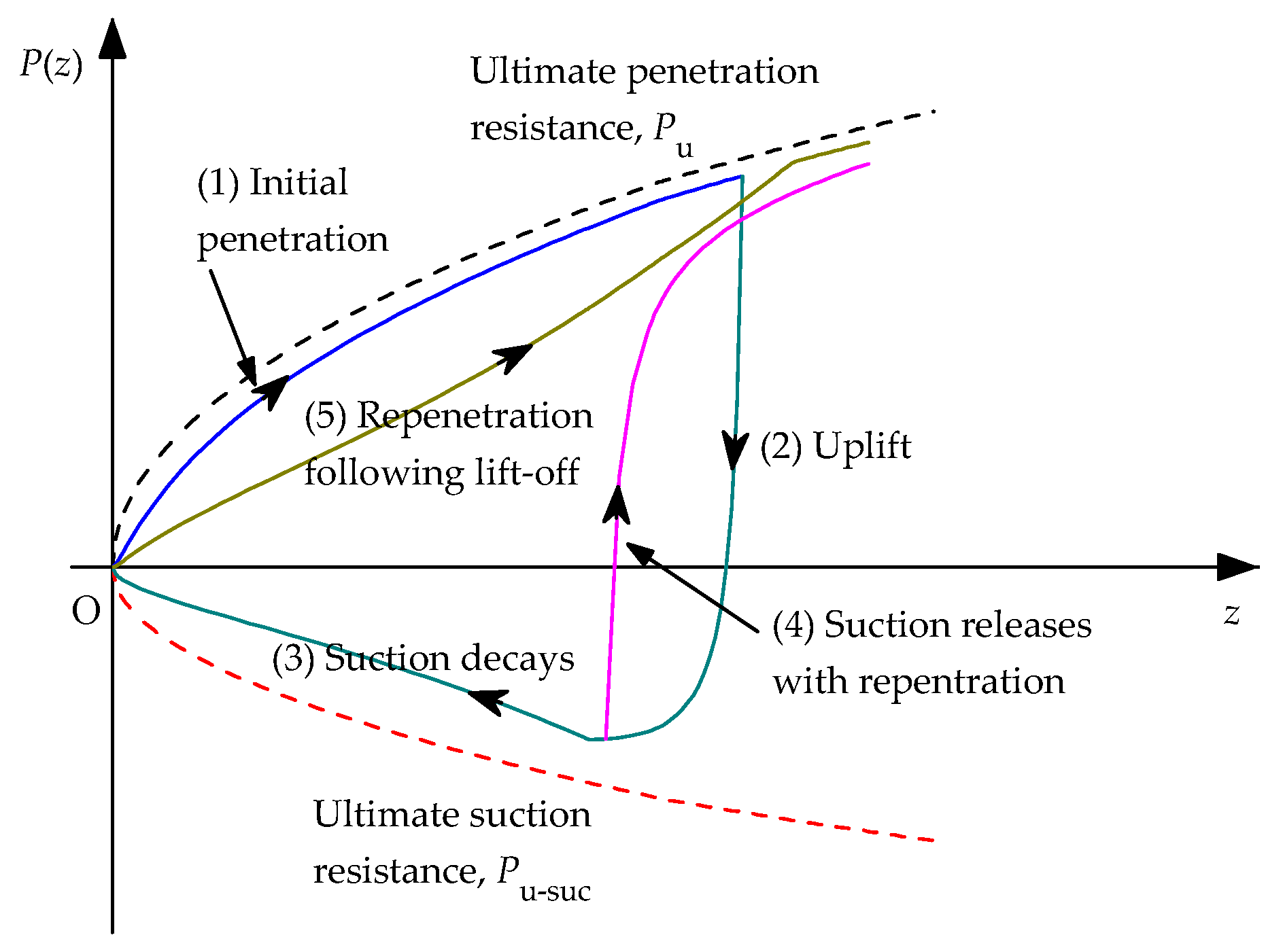
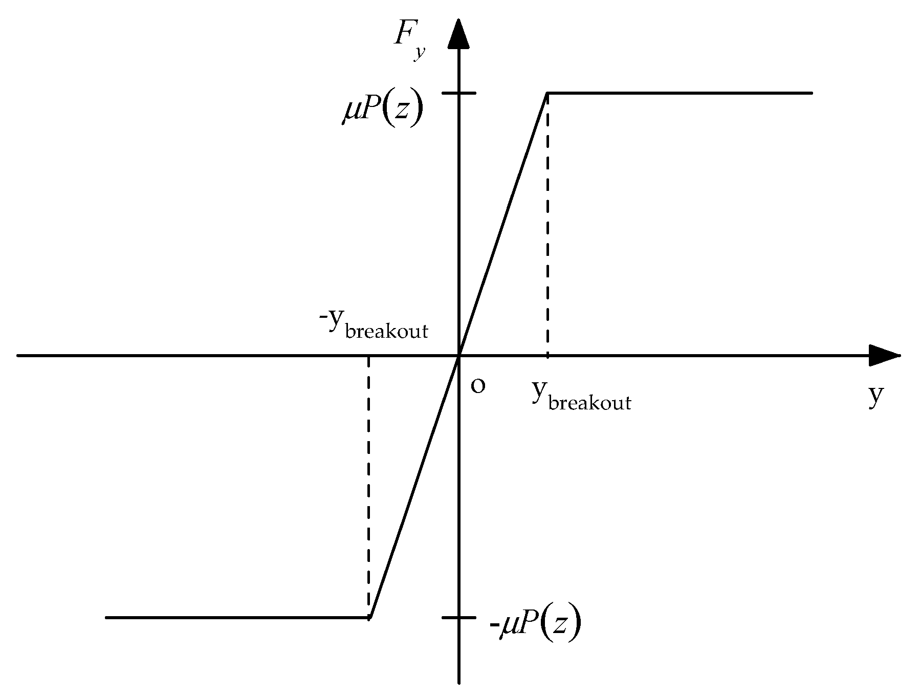
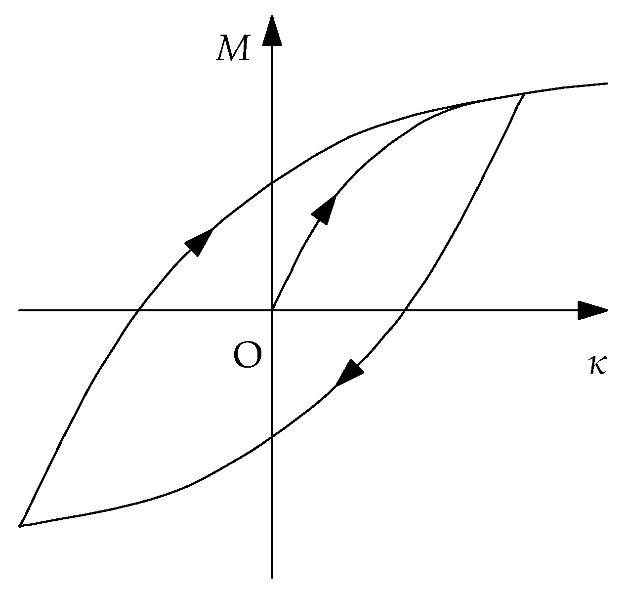
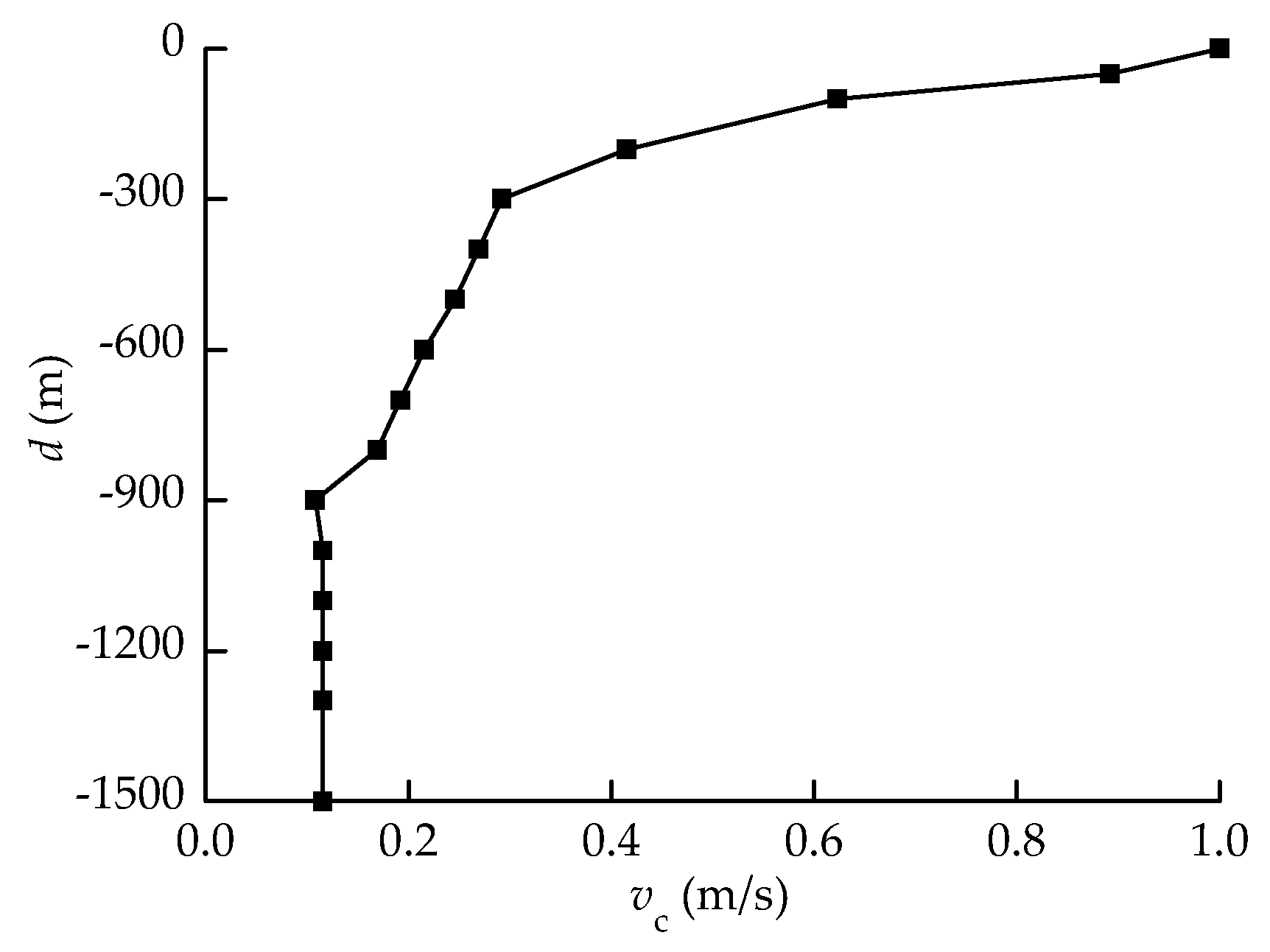
2.3. Pipe–Seabed Soil Interaction

At the touchdown zone (TDZ), the laying pipeline was freely supported by the seabed soil, which was liable to be trenched and remolded under dynamic installation in deep waters. In the vertical plane, the dynamic features of the cyclic pipe–seabed interactions were simulated by a non-linear hysteretic soil model with hyperbolic secant stiffness formulations [29], as shown in Figure 4. In this model, four types of pipe–soil penetration modes were applied to characterize the cyclic variations of the pipeline periodic embedment into the seabed. For the not-in-contact pattern, the seabed resistance P(z) is naturally zero. For other three patterns, including initial penetration, uplift, and repenetration, the relationships between the seabed resistance P(z) and the penetration z non-linearly vary in hysteretic cycles with the incessant shift of the penetration modes.
In another view of the horizontal plane, the lateral and axial pipe–seabed interactions were simulated by the modified Coulomb friction model, which expressed the lateral resistance and axial friction force with the deflection as a bilinear equation, as illustrated in Figure 5. When the lateral displacement y varies from −ybreakout to +ybreakout, the linear friction force is given by F y = k s A y , in which ks refers to the seabed shear stiffness and A represents the contact area. When the lateral displacement y exceeds the range between −ybreakout and +ybreakout, the friction force of the pipe is equal to μ P ( z ) , where P(z) is the vertical seabed resistance and μ is the soil friction coefficient. This model could effectively avoid the discontinuous nature of the friction force at zero lateral displacement and was conveniently implemented in the numerical program [30].

2.4. Pipelay Vessel Motions

According to the geometrical features of the HYSY 201 vessel, a pipelay vessel model was built with a length of 204.65 m and breadth of 39.2 m. The wave frequency motion of the vessel was simulated by use of the displacement response amplitude operators (RAOs), which define the vessel motion responses for each degree of freedom (DoF) to one specified wave direction and wave period. Considering the six DoFs of vessel motions (surge, sway, heave, roll, pitch, and yaw), the motion response spectra of the vessel at the stinger base were derived in light of the RAOs of the HYSY 201 vessel, as illustrated in Figure 6. Almost all six DoFs of the vessel motion responses were greatly noticeable for the quartering seas, in which the heave motion was comparatively remarkable for all seas. It is noted that the slow drift motion of the vessel was restrained to be very small by the advanced dynamic positioning system [31], so it was not taken into consideration in the following analyses due to its small effect on the pipeline dynamic behaviors.

3. Freak Wave Generation

Based on a large amount of ocean observations and laboratory tests, a great many generation models of freak waves have been developed to investigate the phenomenon of rogue wave impact [32,33]. In contrast with the non-linear model, the linear superposition model is simply understood by offshore structure engineers and can be rapidly simulated by researchers. It is also noted that during deepwater installation, the pipeline usually experiences large tension forces of the tensioners, and the influence of hydrodynamic forces induced by non-linear wave factors is very small. A time history train of freak waves must be inserted into the developed installation FEM for the dynamic analysis of an S-lay pipeline. Therefore, the linear superposition technique was employed to generate the freak wave trains.

3.1. Linear Superposition Approach
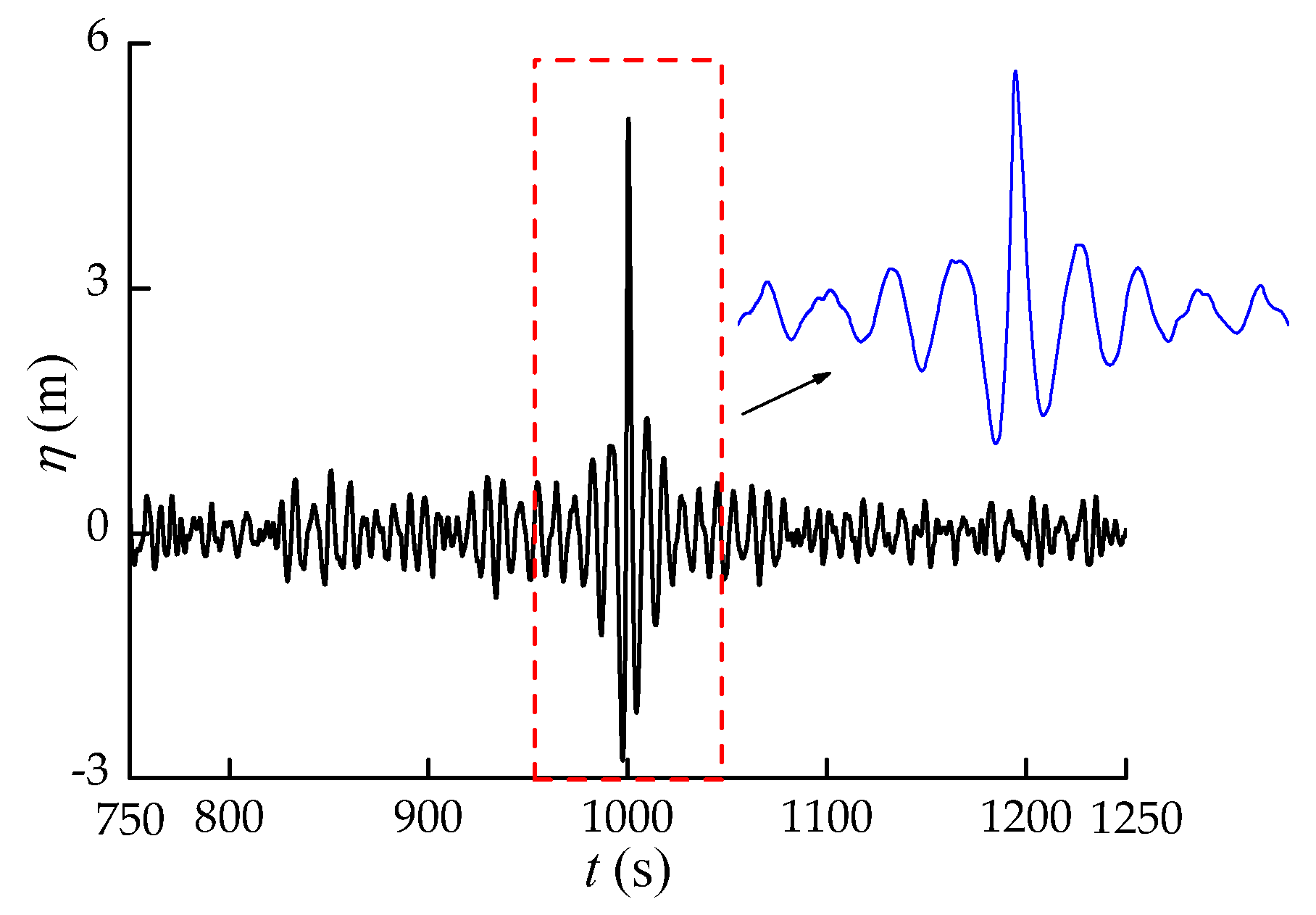
In the linear superposition method, freak waves are described as a combination of transient wave trains with random wave trains for different energy proportions. The transient waves were simulated by the wave focusing model which converges the wave energy of a certain number of wave components at a specified position at the assigned time. The random waves were deemed to be a stationary stochastic process of dispersed energy. The standard JONSWAP spectrum was employed to represent the random sea states in the South China Sea. The generation formula of freak waves can be expressed as
η ( x , t ) = E p 1 i = 1 N [ f i 1 f i 2 S ( f ) d f ] 1 2 cos [ k i ( x x p ) ω i ( t t p ) ] + E p 2 i = 1 N [ f i 1 f i 2 S ( f ) d f ] 1 2 cos [ k i x ω i t + ϕ i ]
where Ep1 and Ep2 are the energy ratio coefficients of transient waves and random waves; the spectral density function is S ( f ) = α g 2 / ( 16 π 4 f 5 ) exp [ 1.25 ( f / f m ) 4 ] γ β ; α is the spectral energy coefficient; and g is the gravitational constant. β = exp [ ( f f m ) 2 / ( 2 τ 2 f m 2 ) ] , in which τ is the spectral width parameter; fm is the peak frequency; γ is the peak enhancement factor; N is the number of wave components; k i , ω i , and ϕ i are the wave number, angular frequency, and phase lag of the ith wave component; and xp and tp are two constants separately representing the focusing position and time of transient waves.

3.2. Case Study

Before the generation of freak waves, there should be a clear mathematical definition. The popularly acceptable criterion for freak waves was adopted in this study, which defines the maximum wave height to be more than two times its significant wave height. Based upon the ocean statistics in the South China Sea, the significant wave height, Hs = 2.0 m, and the peak period, Tp = 8.7 s, were specified for the JONSWAP spectrum, as illustrated in Figure 7. The corresponding peak frequency, fm = 0.115 Hz, and the spectral energy coefficient, α = 0.002, were calculated along with the peak enhancement factor, γ = 3.3. Besides, the spectral width parameter σ was varied with the value of wave frequency. If f ≤ fm, τ = 0.07; otherwise, f > fm, τ = 0.09.
The selected wave spectrum was discretized into 900 components by use of the equal energy approach. These wave components were then gathered in the numerical flume to constitute a sequence of transient wave trains and random wave trains. The energy proportions for both wave trains were set as Ep1 = 0.4 and Ep2 = 0.6, and the distribution range φ of the phase lag was taken as 1.1π. The wave focusing time and position were set at tp = 1000 s and xp = 0 m. Figure 8 illustrates a part of the time history trains of generated freak waves, and the beginning simulation time point was shifted to 750 s with the duration of 500 s so as to cover the maximum wave height in the globe time domain. It can be observed that the freak wave amplitude suddenly surged to a great wave crest of 5.1 m at the focusing time of 1000 s. The maximum wave height attained 7.8 m, which is 3.9 times larger than its significant wave height. The wave time history trains properly reflect the basic characteristic of freak waves in the ocean sea and satisfy the wave amplitude criterion for its definition.

3.3. Sensitive Analysis

The time history trains of freak waves are crucial for the investigation into their effects on the dynamic behaviors of S-laying pipelines. The sensitive analyses of generation factors for the freak wave train must be conducted. Four input parameters, including the wave energy ratio coefficient, focusing position, phase range, and peak value, were selected for the wave simulation by the linear superposition technique. Plenty of freak wave trains were obtained, and a group of represented trains with the duration of 500 s are illustrated in Figure 9. Significant differences in the wave crest and wave trough at the middle time were observed under different initial conditions.
Figure 10 displays the maximum wave heights of freak wave trains with the variation of the initial input parameters. It can be seen that the maximum wave height linearly increases with the increase of the energy ratio coefficient Ep1, which denotes the energy proportion of the transient wave in the freak wave trains. When the focusing location occurred from the distance xp = −200 m to xp = 200 m, the maximum wave height firstly augmented and then reduced, and the crest value attained 7.86 m at the point xp = 0 m. As the phase range added from 1.0π to 1.4π, the maximum wave height gradually decreased. Oppositely, along with the augmentation of the wave peak value from 3.6 to 5.6 m, the maximum wave height linearly magnified.

4. Numerical Implementation of Pipeline Installation under Freak Waves

4.1. Pipelay Parameters

According to a practical engineering case, a 12 inch pipeline was installed into a water depth of 1500 m in the Liwan3-1 (LW3-1) gas field in the South China Sea. The laying pipeline parameters listed in Table 1 were adopted, which included the outer diameter D, wall thickness tp, steel pipe density ρp, elastic modulus E, Poisson’s ratio v, effective yield stress σy, thickness tc and density ρc of the corrosion coatings, weight per unit length in air wa, and submerged weight per unit length ws.
X65 material grade was used for the steel pipe, whose stress–strain relationship curve is displayed in Figure 11 on the basis of the Ramberg–Osgood model. The non-linear relationship between the bending moment and curvature of the steel pipe shown in Figure 12 was obtained by use of the hysteretic bending model, which gave a precise simulation of the bending state of the overbend pipeline under the cyclic clashing contacts with stinger rollers.
The vertical distribution of the current speed among various water depths is illustrated in Figure 13 in light of the field measurement. The current direction was set as 0° in line with the pipelay heading. The ocean current was considered as a two-dimensional steady flow in the vertical plane. The hydrodynamic loads were calculated by means of Morison’s equation [34] and are given by F d = ( Δ a w + C a Δ a r ) + 0.5 C D ρ w A v r | v r | , in which Δ is the mass of fluid displaced by the pipe, αw is the fluid acceleration relative to the earth, Ca is the added mass factor, αr is the fluid acceleration relative to the pipe, CD is the drag coefficient, ρw is the density of sea water, A is the drag area, and νr is the fluid velocity relative to the pipe. For the hydrodynamic calculation, Ca was taken as 1.0, and the CD for the axial and the normal directions was assumed to be 0.024 and 1.2, respectively.
With regard to the non-linear hysteretic soil model applied in this study, a group of seabed soil parameters was selected to describe the basic features of soft clay in the deep water, as listed in Table 2. The ultimate penetration resistance Pu(z) and the nominal bearing capacity factor N c ( z / D ) are non-linearly related to the penetration z and are given by [29]
P u ( z ) = N c ( z / D ) S u ( z ) D
N c ( z / D ) = a ( z / D ) b
where the soil undrained shear strength refers to S u ( z ) = S u 0 + S ug z , in which Su0 is the mudline shear strength and Sug is the shear strength gradient, and a and b are the non-dimensional penetration factors. The saturated soil density ρsoil and normalized maximum stiffness Kmax were taken for the soft clay; other soil model parameters for different penetration patterns were specified as the defaults, including the suction ratio fsuc and the decay factor λsuc, repenetration coefficient λrep and soil buoyancy factor fb. In addition, the seabed soil friction coefficient μ and shear stiffness ks were adopted for the simulation of axial and lateral pipe–seabed interactions [35].

4.2. Calcultion Method

The dynamic calculation of laying pipeline responses induced by freak waves contained two modules: one was the S-lay model and another was the freak wave train. Firstly, a global S-lay model with the framework of OrcaFlex was established at a water depth of 1500 m. This model comprised the pipelay vessel, tensioner, stinger, pipeline, and seabed. Under the combined actions of self-weight, buoyancy, and internal forces, the equilibrium positions of the laying pipeline from the tensioner on the vessel via the stinger to the seabed were initially determined by utilization of the catenary technique. Subsequently, the hysteretic bending stiffness and the clashing mutual contacts of pipe-stinger rollers were further taken into account to obtain the full equilibrium configurations of the pipeline. The final static results of the S-lay system were taken as the initial values of the dynamic simulation.
Based upon the linear superposition technique, a series of time history trains of freak waves were obtained from the MATLAB program. These freak wave trains were then inserted into the developed S-lay model as the input conditions of extreme sea states. The geometric non-linearities of the laying pipeline, spatial variations of hydrodynamic forces, and clashing contacts were sufficiently incorporated in the simulation. The time domain calculations of the S-lay system under freak waves were conducted by use of the explicit dynamic integration approach. Besides, critical damping and target damping were utilized to cut down the spurious non-physical high frequency responses, and they were demonstrated to have little effect on the pipeline behaviors. Finally, the whole motion equations for the vessel and all line nodes were solved by iterative update of the forces and moments on the nodes and segments at each time step.

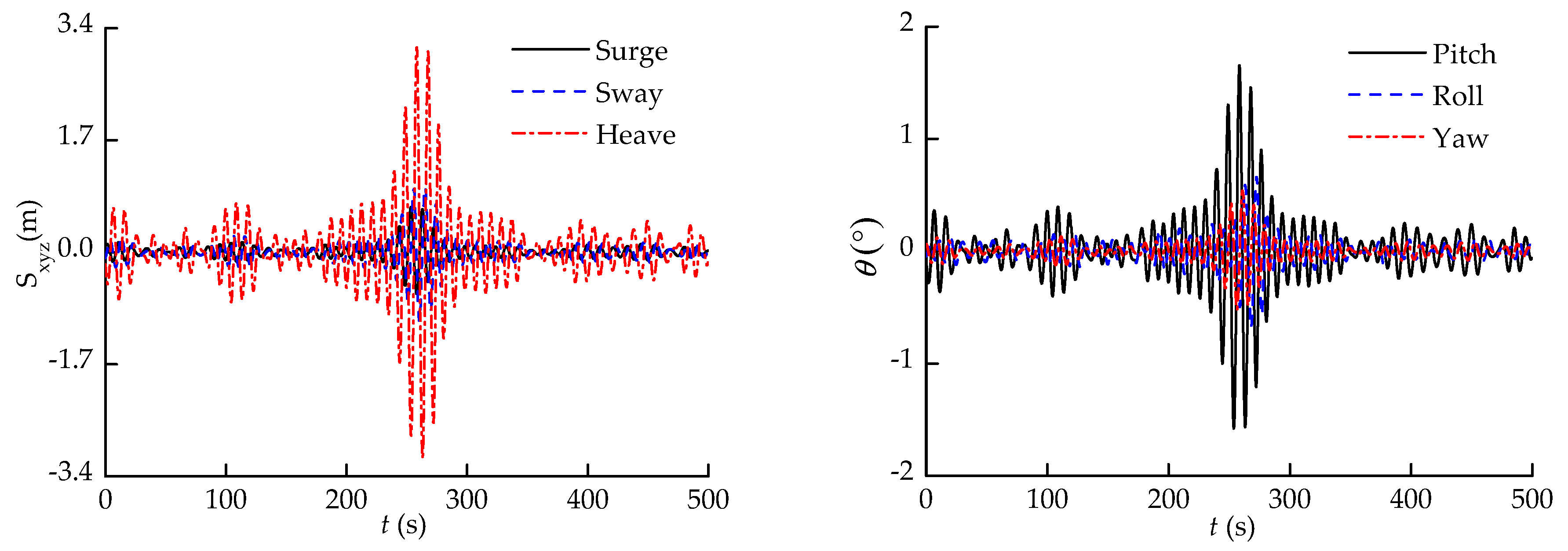
4.3. Time History Response of Pipelay Vessel Motions

The pipelay vessel motions are significant top excitation boundaries of the S-laying pipeline and cause dynamic responses. Under the generated freak wave trains shown in Figure 8 for the extreme quartering sea, the time history responses of six DoFs of pipelay vessel motions were calculated by use of displacement RAOs, as displayed in Figure 14. The heave motion among vessel translation responses was more prominent than the surge and the sway motion, and the pitch motion among vessel rotation responses was larger than the roll and the yaw motion. These results validate the above-mentioned response spectra of the pipelay vessel. Moreover, all six DoFs of the vessel motion response amplitudes abruptly rose and attained maximum values near the middle time of 250 s, which also reflects the basic time history characteristic of freak waves.

5. Results Analysis

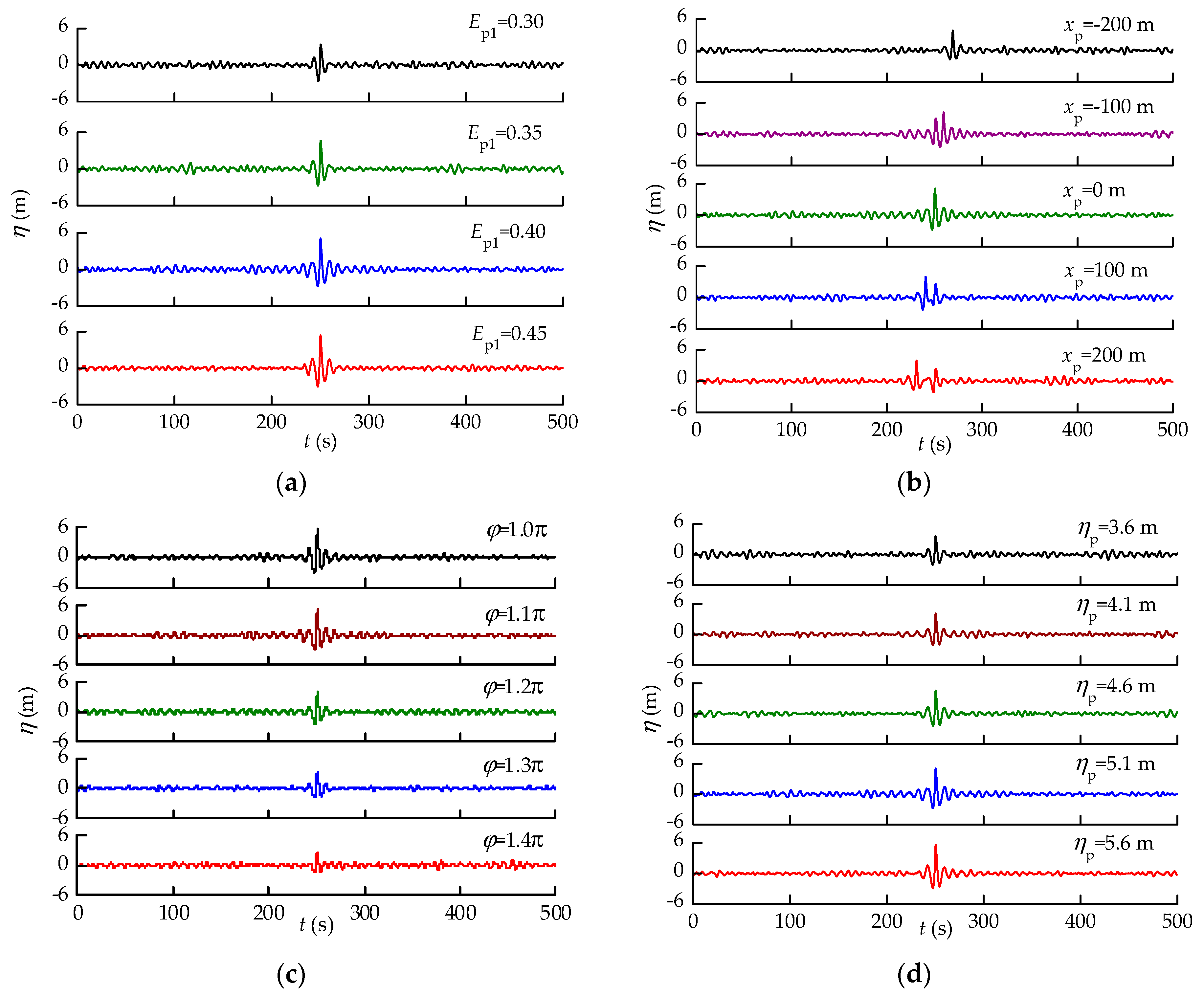
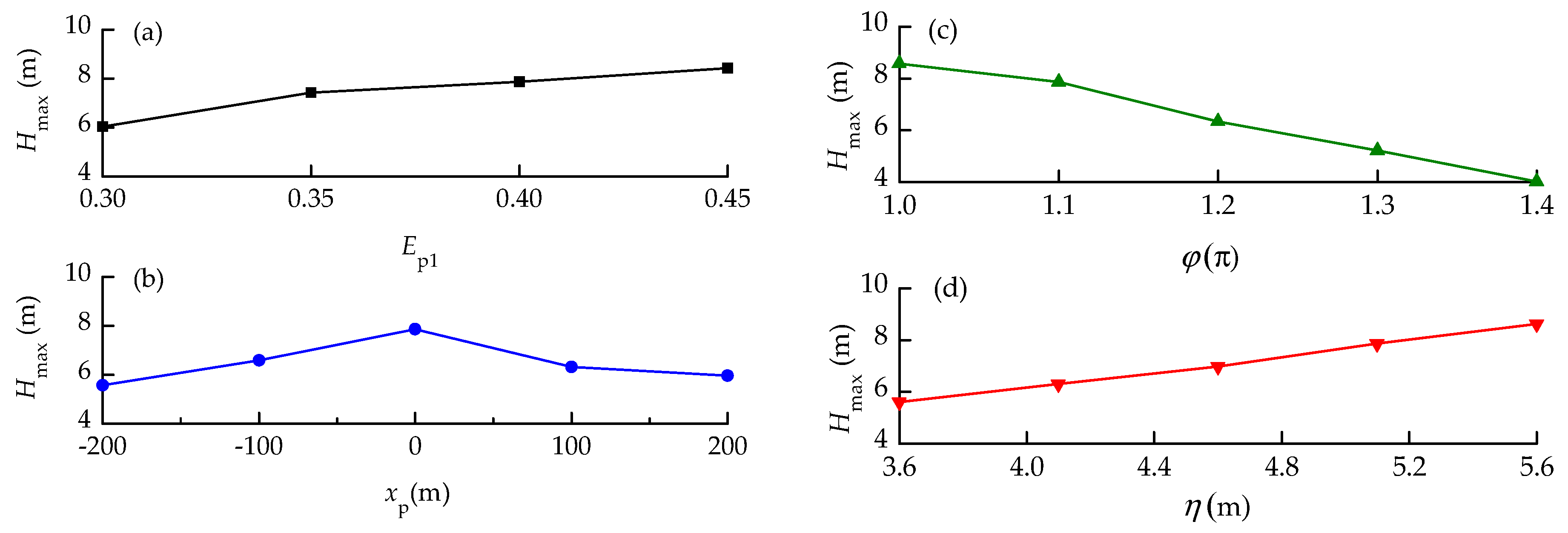
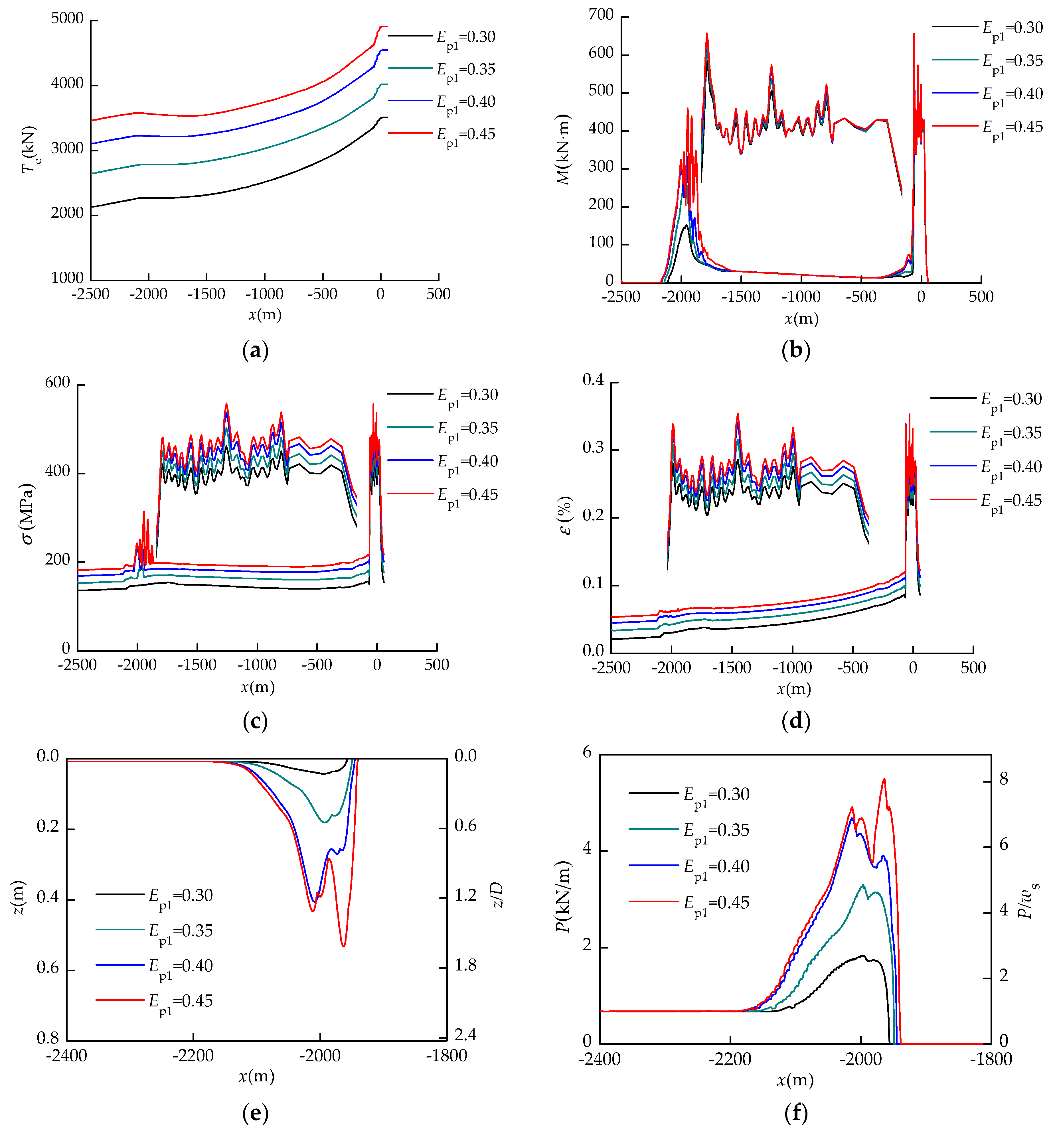
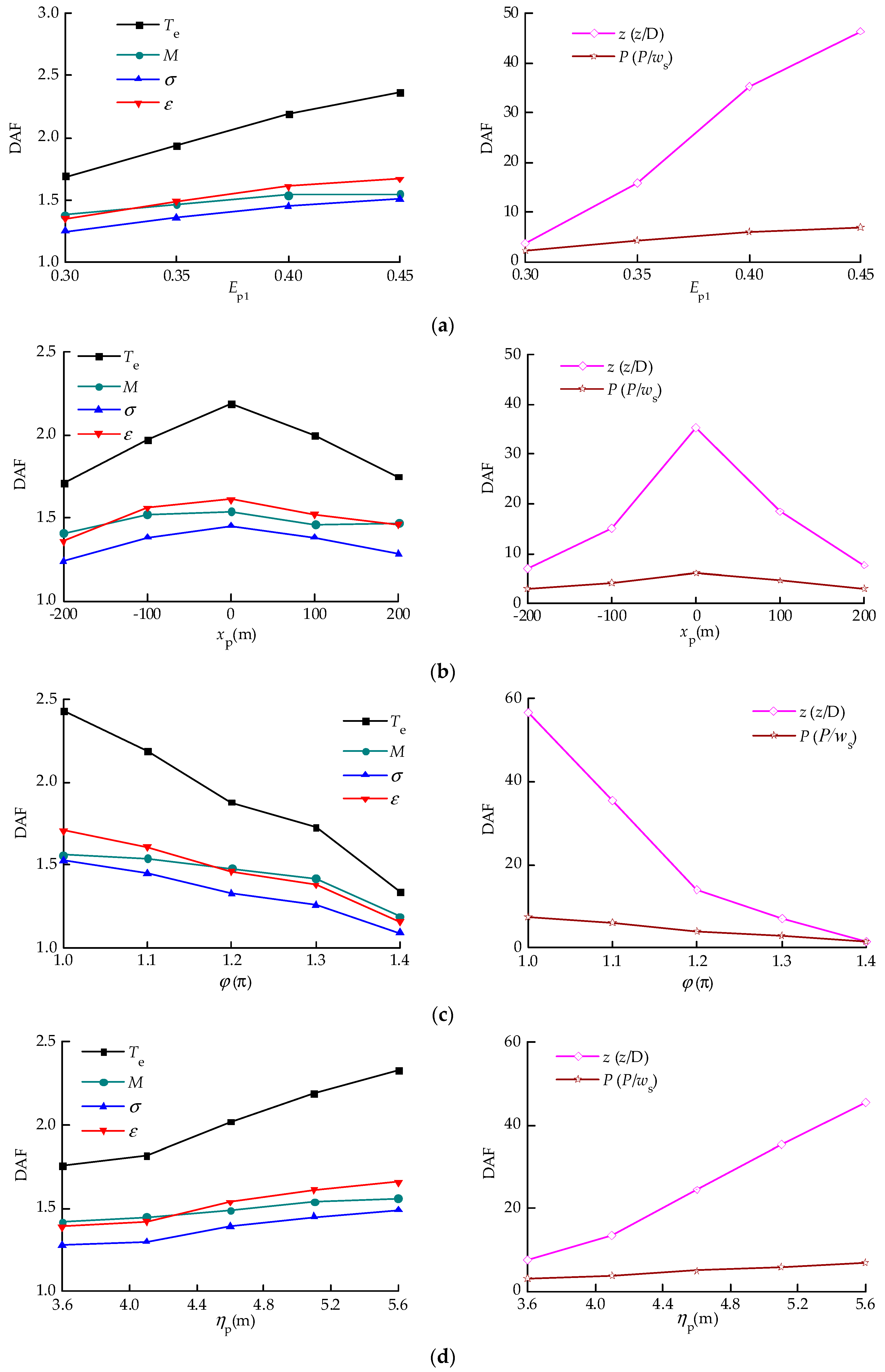
5.1. Effect of the Wave Energy Ratio Coefficient

In the simulation of freak wave trains, the energy ratio coefficient directly dominates the energy proportion of transient waves and random waves. By selecting four energy ratio coefficients, Ep1 = 0.30, 0.35, 0.40 and 0.45, a group of freak wave trains in Figure 9a was utilized as the input marine environment conditions for the dynamic analyses of the S-laying pipeline. The pipeline and seabed response results, which includes the axial tension, bending moment, von Mises stress, longitudinal strain, pipeline embedment, and seabed resistance, are illustrated in Figure 15.
As the energy ratio coefficient Ep1 increased from 0.30 to 0.45, the axial tension of the overall pipeline noticeably rose, and its maximum value at the top end increased by 39.9% from 3512.57 to 4915.02 kN. The bending moments of the pipeline had some differences between the overbend and the sagbend, and the maximum results appeared at the last contact roller location in the overbend with a minor increase of 12.1% from 585.86 to 656.95 kN·m. In the sagbend, the maximum bending moment occurring near the touchdown point (TDP) had a prominent augmentation of 202.3% from 151.97 to 459.33 kN·m, and some bending moment crests along the touchdown pipeline formed as a result of pipe bending and soil softening. Under the combined axial tension, bending moment, and hydrostatic force, the von Mises stress of the pipeline increased to some extent and attained 20.8% of the maximum value from 461.27 to 557.10 MPa. Similarly, the maximum longitudinal strain of the pipeline rose by 23.9% from 0.285% to 0.353%. Moreover, the maximum pipeline embedment had a remarkable enlargement of 1139.5% from 0.043 (0.130D) to 0.533 m (1.616D), and the maximum seabed resistance grew by 199.8% from 1.837 (2.701ws) to 5.507 kN/m (8.097ws). It is demonstrated from these results that the energy ratio coefficient has an obvious effect on the pipeline dynamic behaviors and seabed resistance. Especially, when the Ep1 reaches 0.45, the freak wave causes drastic dynamic responses of the pipeline and seabed interaction in the TDZ.

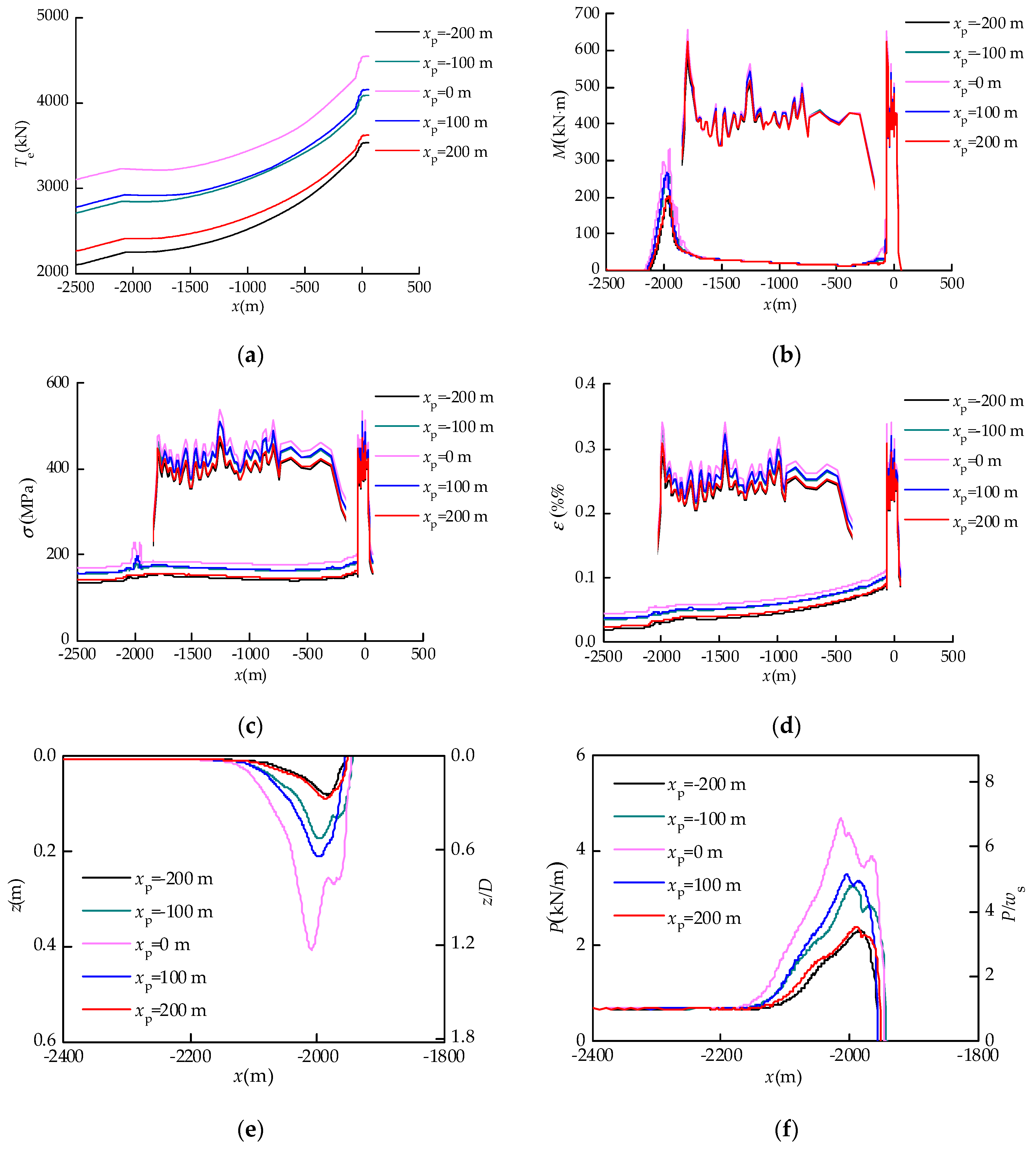
5.2. Effect of the Wave Focusing Location

A noticeable characteristic of freak waves is the crest value appearing at the focusing position where the wave energy accumulates. To explore the influence of the wave focusing location on the dynamic responses of the laying pipeline, five focusing locations, xp = −200, −100, 0, 100, 200 m, were assumed to simulate the freak waves shown in Figure 9b, which were separately taken as the input surface wave conditions to perform a dynamic analysis of pipeline installation. The pipeline and seabed response results illustrated in Figure 16 are the axial tension, bending moment, von Mises stress, longitudinal strain, pipeline embedment, and seabed resistance.
When the wave focusing location varied from −200 m to 200 m, the pipeline and seabed responses firstly rose and then dropped. The maximum responses occurred at the center position xp = 0 m with a peak axial tension of 4550.13 kN, bending moment of 654.13 kN·m, von Mises stress of 536.49 MPa, longitudinal strain of 0.340%, pipeline embedment of 0.406 m (1.231D), and seabed resistance of 4.685 kN/m (6.889ws). The pipeline responses and seabed resistance at xp = 100 m and xp = 200 m were slightly larger than the corresponding results at xp = −100 m and xp = −200 m, for which the freak waves produced by the forward focusing location led to more prominent motion responses of the pipelay vessel. Evidently, the dynamic behaviors of the laying pipeline and seabed resistance are greatly influenced by the wave focusing location.

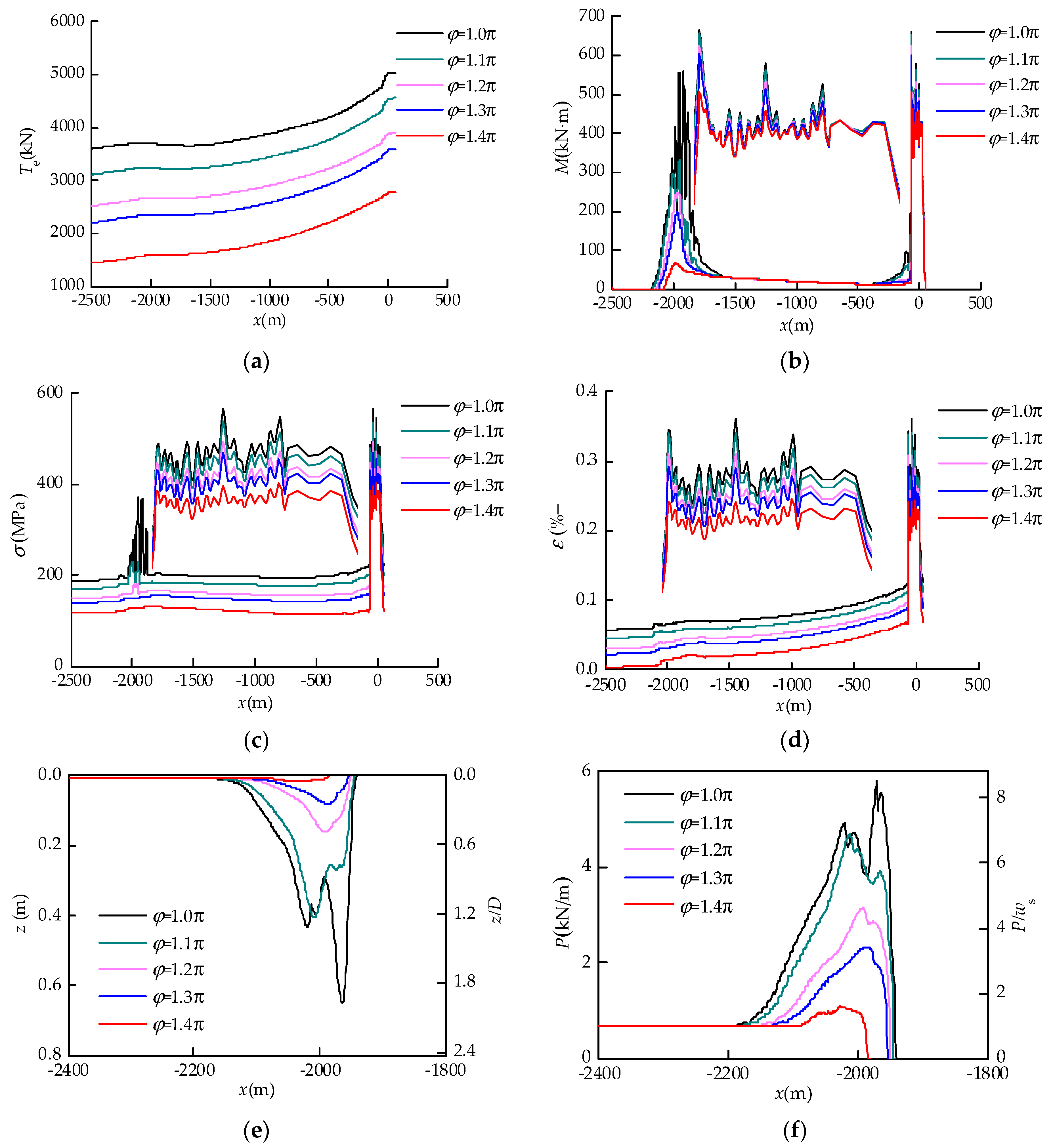
5.3. Effect of the Wave Phase Range

The wave phase range plays a significant role in generating freak waves and, to some degree, determines the wave height by controlling the phases of wave components in a specified region. Five groups of the wave phase range, φ = 1.0π, 1.1π, 1.2π, 1.3π and 1.4π, were selected to produce the freak wave trains shown in Figure 9c, and the influence of the wave phase range on the pipeline behaviors was explored by the combination of these wave trains with the developed S-lay FEM for time domain dynamic analyses. The pipeline and seabed response results on aspects of axial tension, bending moment, von Mises stress, longitudinal strain, pipeline embedment, and seabed resistance are displayed in Figure 17.
With the increase of the wave phase range from 1.0π to 1.4π, all the pipeline and seabed responses had prominent decreases. The reductions in the maximum values were 45.0% for the axial tension, from 5034.62 to 2769.11 kN; 23.6% for the bending moment, from 661.99 to 506.08 kN·m; 29.0% for the von Mises stress, from 565.67 to 401.41 MPa; and 32.4% for the longitudinal strain, from 0.361% to 0.244%. Moreover, the maximum pipeline embedment reduced by 97.2%, from 0.649 (1.967D) to 0.018 m (0.055D), and the maximum seabed resistance dropped by 81.1%, from 5.793 (8.518ws) to 1.097 kN/m (1.613ws). When the wave phase range was 1.0π, the bending moment and von Mises stress of the pipeline in the TDZ tremendously jumped to form some crests, as illustrated in Figure 17b,c. This phenomenon can be explained from the peak curves of pipeline embedment and seabed resistance shown in Figure 17e,f as the cyclic motions of the pipeline penetrating into and uplifting from the seabed, resulting in the softening and trenching of seabed soil, and the drastic pipe–seabed interactions induced by freak waves causing great pipeline flexural deflections. These results adequately demonstrate that the phase range of freak waves greatly influences the dynamic behaviors of the pipeline and the seabed, particularly for the entire axial tension and pipeline embedment as well as seabed resistance in the TDZ.

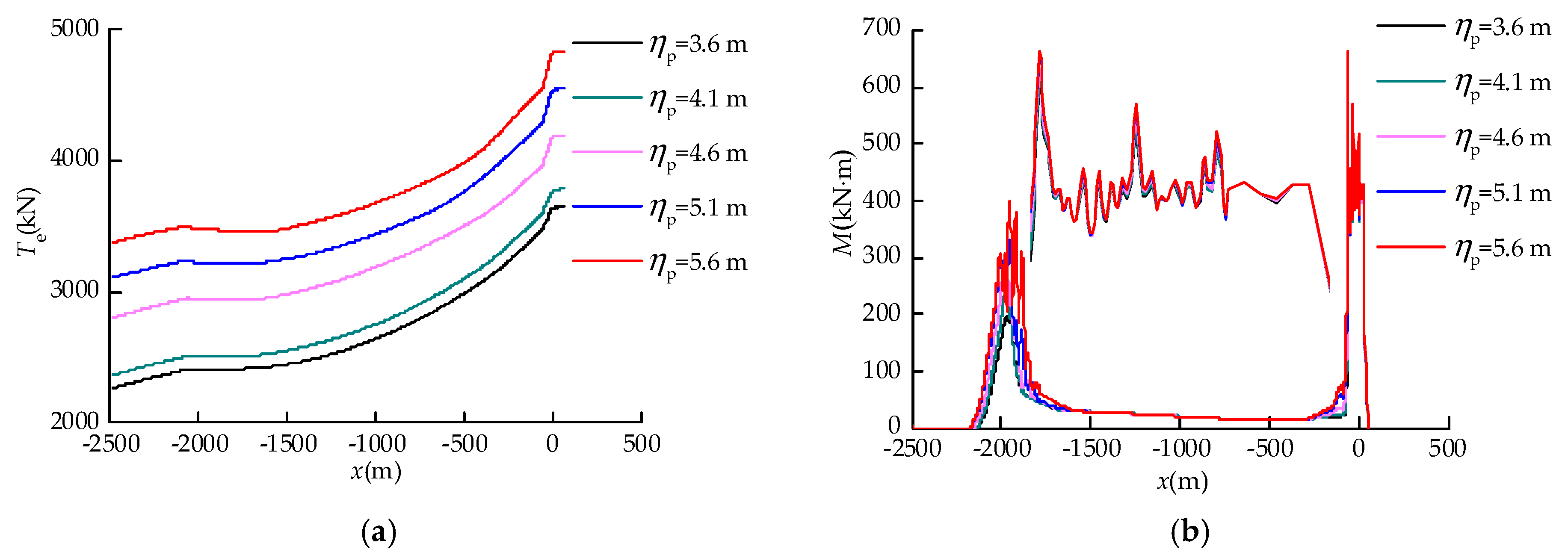
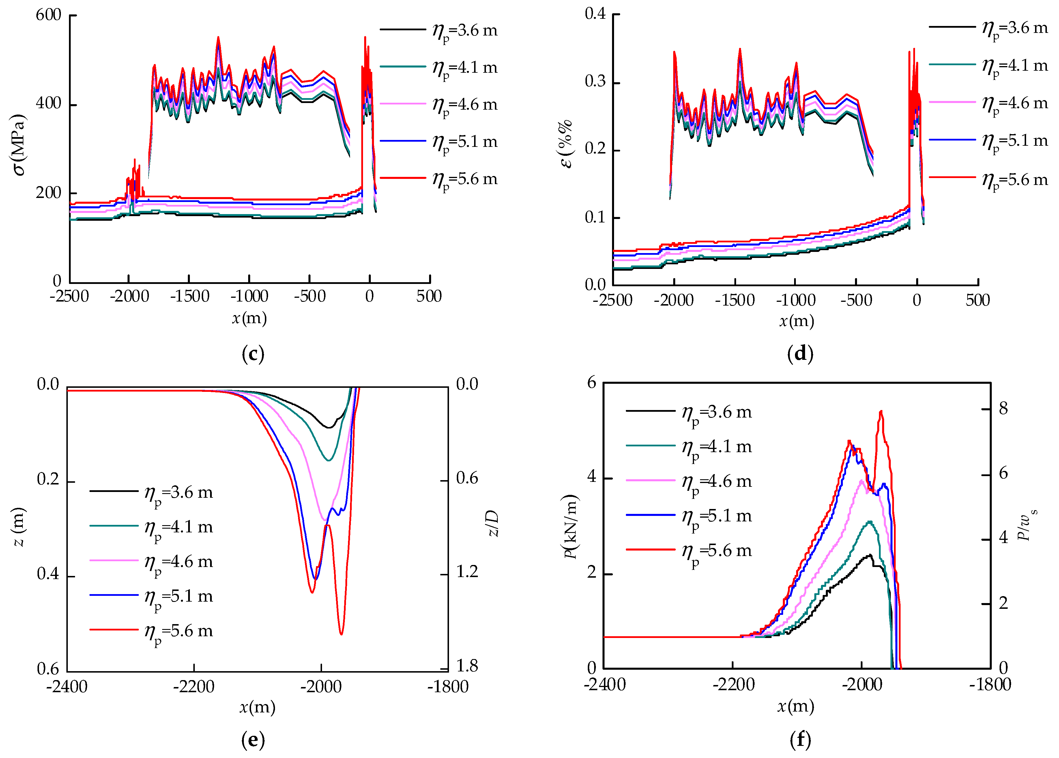
5.4. Effect of Wave Peak Value

Another noteworthy feature of freak waves is the peak value which generally represents the impact levels on offshore structures. In order to better understand the wave peak value effect on the dynamic behaviors of the S-laying pipeline, the five representative freak wave trains shown in Figure 9d were generated with their corresponding wave peak values of 3.6, 4.1, 4.6, 5.1, and 5.6 m. A time domain analysis of pipeline installation under these freak waves was conducted to obtain the pipeline and seabed response results, as shown in Figure 18.
Since the wave peak value gradually became larger from 3.6 to 5.6 m, all the pipeline and seabed responses showed an obvious increase. The axial tension of the overall pipeline became greater, and the maximum tension enlarged by 32.6%, from 3647.71 to 4838.41 kN. The bending moment of the pipeline mildly increased by 9.7% for its maximum value, from 602.24 to 660.69 MPa, in the overbend. Meanwhile, the bending moment in the sagbend had a great increase with the increment of its maximum value, attaining 103.2%, from 197.25 to 400.83 kN·m. Likewise, the maximum von Mises stress of the pipeline rose by 17.1%, from 471.98 to 552.47 MPa, and the maximum longitudinal strain of the pipeline rose by 19.5%, from 0.293% to 0.350%. Additionally, the maximum pipeline embedment and seabed resistance remarkably enlarged by 507.0% and 127.3%, respectively, from 0.086 (0.261D) to 0.522 m (1.582D) and from 2.387 (3.510ws) to 5.426 kN/m (7.978ws). Therefore, the increase in the freak wave peak value would result in great augmentation of pipeline behaviors and seabed resistance.

6. Discussion and Implications

The deepwater S-lay FEM is a complicated, non-linear structural system, and dynamic response analysis of the laying pipeline under freak waves is difficult and time-consuming for marine structure engineers. A simplified technique was presented to estimate the pipeline dynamic response amplitudes by means of the dynamic amplification factors (DAFs), which are defined by the maximum responses relative to the corresponding static results. As a consequence, the dynamic response amplitudes of the laying pipeline can be easily determined if the static responses and DAFs are given.
As shown in Figure 19a, the pipeline and seabed DAFs in the parametric analyses were obtained with the variation of the energy ratio coefficient. Along with the increase of the energy ratio coefficient Ep1, the DAFs of axial tension, bending moment, stress, and strain gradually increased, in which the tension DAF was relatively prominent from 1.69 to 2.37. The pipeline embedment DAF largely rose from 3.75 to 46.41, and the seabed resistance DAF increased from 2.35 to 7.04. Figure 19b shows the variation in pipeline and seabed DAFs with the wave focused position, and all the DAFs firstly rose up and then dropped down. The maximum tension DAF reached 2.19, and the maximum pipeline embedment and seabed resistance DAFs reached 35.35 and 5.99, respectively. Moreover, the pipeline and seabed DAFs with the variation in the wave phase range are illustrated in Figure 19c. As the wave phase range increased, all of the DAFs reduced step by step. The DAF reductions were from 2.43 to 1.34 for axial tension, from 56.50 to 1.57 for pipeline embedment, and from 7.40 to 1.40 for seabed resistance. Oppositely, the pipeline and seabed DAFs enlarged stage by stage with the augmentation of the wave peak value, as displayed in Figure 19d, the DAF increment in axial tension was from 1.42 to 1.56, and the DAF increments in pipeline embedment and seabed resistance were from 7.49 to 45.44 and from 3.05 to 6.93. These obtained DAFs of the pipeline and seabed behaviors could offer intuitional knowledge for offshore pipeline engineers, which could be used to consider the freak wave effects in the initial design stage.

7. Conclusions

This paper presented a profound investigation of freak wave effects on the dynamic responses of offshore pipelines for deepwater installation. For this purpose, an extended FEM of the S-lay system was developed in OrcaFlex with the particular consideration of freak waves. The linear superposition method of combined transient wave trains and random wave trains was applied to generate a series of freak wave trains. The wave induced pipelay vessel motions, pipe–stinger roller interactions in the overbend, as well as the cyclic contacts between the pipeline and seabed in the TDZ were also taken into account in the dynamic analysis of laying pipelines. The influences of the freak wave energy ratio coefficient, focusing location, phase range, and peak value on the pipeline and seabed behaviors were estimated in detail, and the DAFs of the axial tension, bending moment, von Mises stress, longitudinal strain, pipeline embedment, and seabed resistance were derived. Some significant conclusions were obtained as follows:
(1)
The reasonable selection of wave parameters can effectively generate a variety of freak wave trains by the linear superposition model. The maximum heights of freak wave trains are obviously different with variations in the energy ratio coefficient, focusing position, phase range, and peak value. The freak wave trains could be steadily incorporated into the developed S-lay FEM to implement the dynamic analysis of deepwater pipeline installation.
(2)
The energy ratio coefficient has a great influence on the generation of freak waves and the induced pipeline dynamic responses. With an increase in the energy ratio coefficient for transient waves, all the pipeline behaviors and seabed resistance remarkably increase. Especially, when the Ep1 reaches 0.45, the interaction responses of the touchdown pipeline and seabed soil are drastically noticeable, which causes tremendous variation in the bending moment, von Mises stress, and pipeline embedment in the TDZ.
(3)
The dynamic behaviors of the laying pipeline and seabed resistance are also strongly influenced by the wave focusing location. When the focusing wave is located at the center position xp = 0 m, the responses of the offshore pipeline and seabed resistance are the most significant. Besides, the axial tension, pipeline embedment, and seabed resistance for the forward wave focusing location are slightly larger than the corresponding results for the negative wave focusing location.
(4)
The phase range and peak value of freak waves were proven to be important influencing factors in the pipeline and seabed responses. As the wave phase range increases, the axial tension, bending moment, von-Mises stress, longitudinal strain, pipeline embedment, and seabed resistance as well as their DAFs remarkably decrease. On the contrary, when the wave peak value becomes larger, the pipeline behaviors and seabed resistance obviously augment.

Author Contributions

Conceptualization, P.X. and S.G.; methodology, P.X. and S.G.; software, P.X.; validation, P.X.; formal analysis, P.X. and Z.D.; investigation, P.X. and Z.D.; resources, P.X. and S.G.; data curation, Z.D.; writing—original draft preparation, P.X. and Z.D.; supervision, S.G.; funding acquisition, P.X. and S.G. All authors have read and agreed to the published version of the manuscript.

Funding

This research was funded by the National Natural Science Foundation of China (grant numbers 51809048, 51779223) and the Natural Science Foundation of Fujian Province, China (grant number 2018J05081).

Acknowledgments

The authors would like to thank the anonymous reviewers for their constructive comments and suggestions.

Conflicts of Interest

The authors declare no conflict of interest.

Nomenclature

Aiinternal cross-section area
Aoexternal cross-section area
Bcoefficient of the Ramberg–Osgood model
Caadded mass coefficient
CDdrag coefficient
dshortest separation distance of the center lines between the pipe and roller
Dpipe outer diameter
Eelastic modulus
Ep1energy ratio coefficient of a transient wave
Ep2energy ratio coefficient of a random wave
EAnomnominal axial stiffness
fmpeak frequency
ggravitational constant
k1pipe contact stiffness
k2roller contact stiffness
kiwave number of the ith wave component
Kmaxsoil normalized maximum stiffness
kssoil shear stiffness
Linstantaneous length of a line segment
L0unstretched length of a line segment
Mbbending moment
npower exponent of the Ramberg–Osgood model
Nnumber of wave components
Ncsoil nominal bearing capacity factor
Piinternal pressure
Poexternal pressure
Pu(z)soil ultimate penetration resistance
r1pipe radius
r2roller radius
S(f)spectral density function
Su0soil mudline shear strength
Sugsoil shear strength gradient
tccorrosion coating thickness
tpwave focusing time
tppipe wall thickness
Teeffective tension
Twwall tension
Tortorque moment
wapipe weight per unit length in air
wspipe submerged weight per unit length
xpwave focusing position
αspectral energy coefficient
γpeak enhancement factor
κ2curvature
μsoil friction coefficient
νPoisson’s ratio
ρcpipe corrosion coating density
ρppipe density
ρsoilsaturated soil density
ρwsea water density
ω i angular frequency of the ith wave component
ϕ i phase lag of the ith wave component
σ y effective yield stress
φtwist angle
τspectral width parameter
ξaxial damping coefficient
ςbending damping coefficient
ζtorsional damping coefficient

References

  1. Kjeldsen, S.P. Measurements of freak waves in Norway and related ship accidents. In Proceedings of the Royal Institution of Naval Architects International Conference-Design and Operation for Abnormal Conditions III, London, UK, 29–30 April 2004. [Google Scholar]
  2. Slunyaev, A.; Didenkulova, I.; Pelinovsky, E. Rogue waves in 2006–2010. Nat. Hazards Earth Syst. Sci. 2011, 11, 2913–2924. [Google Scholar]
  3. Bruschi, R.; Vitali, L.; Marchionni, L.; Parrella, A.; Mancini, A. Pipe technology and installation equipment for frontier deep water projects. Ocean Eng. 2015, 108, 369–392. [Google Scholar] [CrossRef]
  4. Davis, M.C.; Zarnick, E.E. Testing ship models in transient waves. In Proceedings of the 5th International Symposium on Naval Hydrodynamics, Bergen, Norway, 10–12 September 1964; David Taylor Model Basin Hydromechanics Lab: Washington, DC, USA, 1964. [Google Scholar]
  5. Baldock, T.E.; Swan, C.; Taylor, P.H. A laboratory study of nonlinear surface wave in water. Philos. Trans. Math. Phys. Eng. Sci. 1996, 354, 649–676. [Google Scholar]
  6. Fochesato, C.; Grilli, S.; Dias, F. Numerical modeling of extreme rogue waves generated by directional energy focusing. Wave Motion 2007, 44, 395–416. [Google Scholar] [CrossRef]
  7. Zhao, X.Z.; Sun, Z.C.; Liang, S.X. Efficient focusing models for generation of freak waves. China Ocean Eng. 2009, 23, 429–440. [Google Scholar]
  8. Zhao, X.Z.; Ye, Z.T.; Fu, Y.N.; Cao, F.F. A CIP-based numerical simulation of freak wave impact on a floating body. Ocean Eng. 2014, 87, 50–63. [Google Scholar] [CrossRef]
  9. Liu, Z.Q.; Zhang, N.C.; Yu, Y.X. An efficient focusing model for generation of freak waves. Acta Oceanol. Sin. 2011, 30, 19–26. [Google Scholar] [CrossRef]
  10. Hu, Z.Q.; Tang, W.Y.; Xue, H.X. A probability-based superposition model of freak wave simulation. Appl. Ocean Res. 2014, 47, 284–290. [Google Scholar] [CrossRef]
  11. Tang, Y.G.; Li, Y.; Wang, B.; Liu, S.X.; Zhu, L.H. Dynamic analysis of turret-moored FPSO system in freak wave. China Ocean Eng. 2016, 30, 521–534. [Google Scholar] [CrossRef]
  12. Pan, W.B.; Zhang, N.C.; Huang, G.X.; Ma, X.Y. Experimental study on motion responses of a moored rectangular cylinder under freak waves (I: Time-domain study). Ocean Eng. 2018, 153, 268–281. [Google Scholar] [CrossRef]
  13. Gong, S.F.; Chen, K.; Chen, Y.; Jin, W.L.; Li, Z.G.; Zhao, D.Y. Configuration analysis of deepwater S-lay pipeline. China Ocean Eng. 2011, 25, 519–530. [Google Scholar] [CrossRef]
  14. Marchionni, L.; Alessandro, L.; Vitali, L. Offshore pipeline installation: 3-dimensional finite element modelling. In Proceedings of the 30th International Conference on Offshore Mechanics and Arctic Engineering, Rotterdam, The Netherlands, 19–24 June 2011. [Google Scholar]
  15. O’Grady, R.; Harte, A. Localised assessment of pipeline integrity during ultra-deep S-lay installation. Ocean Eng. 2013, 68, 27–37. [Google Scholar] [CrossRef]
  16. Gong, S.F.; Xu, P.; Bao, S.; Zhong, W.J.; He, N.; Yan, H. Numerical modelling on dynamic behaviour of deepwater S-lay pipeline. Ocean Eng. 2014, 88, 393–408. [Google Scholar] [CrossRef]
  17. Gong, S.F.; Xu, P. The influence of sea state on dynamic behaviour of offshore pipelines for deepwater S-lay. Ocean Eng. 2016, 111, 398–413. [Google Scholar] [CrossRef]
  18. Ivić, S.; Čanađija, M.; Družeta, S. Static structural analysis of S-lay pipe laying with a tensioner model based on the frictional contact. Eng. Rev. 2014, 34, 223–234. [Google Scholar]
  19. Ivić, S.; Družeta, S.; Hreljac, I. S-Lay pipe laying optimization using specialized PSO method. Struct. Multidiscip. Optim. 2017, 56, 297–313. [Google Scholar] [CrossRef]
  20. Xie, P.; Zhao, Y.; Yue, Q.J.; Palmer, A.C. Dynamic loading history and collapse analysis of the pipe during deepwater S-lay operation. Mar. Struct. 2015, 40, 183–192. [Google Scholar] [CrossRef]
  21. Cabrera-Miranda, J.M.; Paik, J.K. On the probabilistic distribution of loads on a marine riser. Ocean Eng. 2017, 134, 105–118. [Google Scholar] [CrossRef]
  22. Wang, F.C.; Chen, J.; Gao, S.; Tang, K.; Meng, X.W. Development and sea trial of real-time offshore pipeline installation monitoring system. Ocean Eng. 2017, 146, 468–476. [Google Scholar] [CrossRef]
  23. Liang, H.; Yue, Q.J.; Lim, G.; Palmer, A.C. Study on the contact behaviour of pipe and rollers in deep S-lay. Appl. Ocean Res. 2018, 72, 1–11. [Google Scholar] [CrossRef]
  24. Liang, H.; Zhao, Y.; Yue, Q.J. Experimental study on dynamic interaction between pipe and rollers in deep S-lay. Ocean Eng. 2019, 175, 188–196. [Google Scholar] [CrossRef]
  25. Kim, H.S.; Kim, B.W. An efficient linearised dynamic analysis method for structural safety design of J-lay and S-lay pipeline installation. Ships Offshore Struct. 2019, 14, 204–219. [Google Scholar] [CrossRef]
  26. Orcina. OrcaFlex User Manual, Version 9.7a; Orcina: Cumbria, UK, 2014. [Google Scholar]
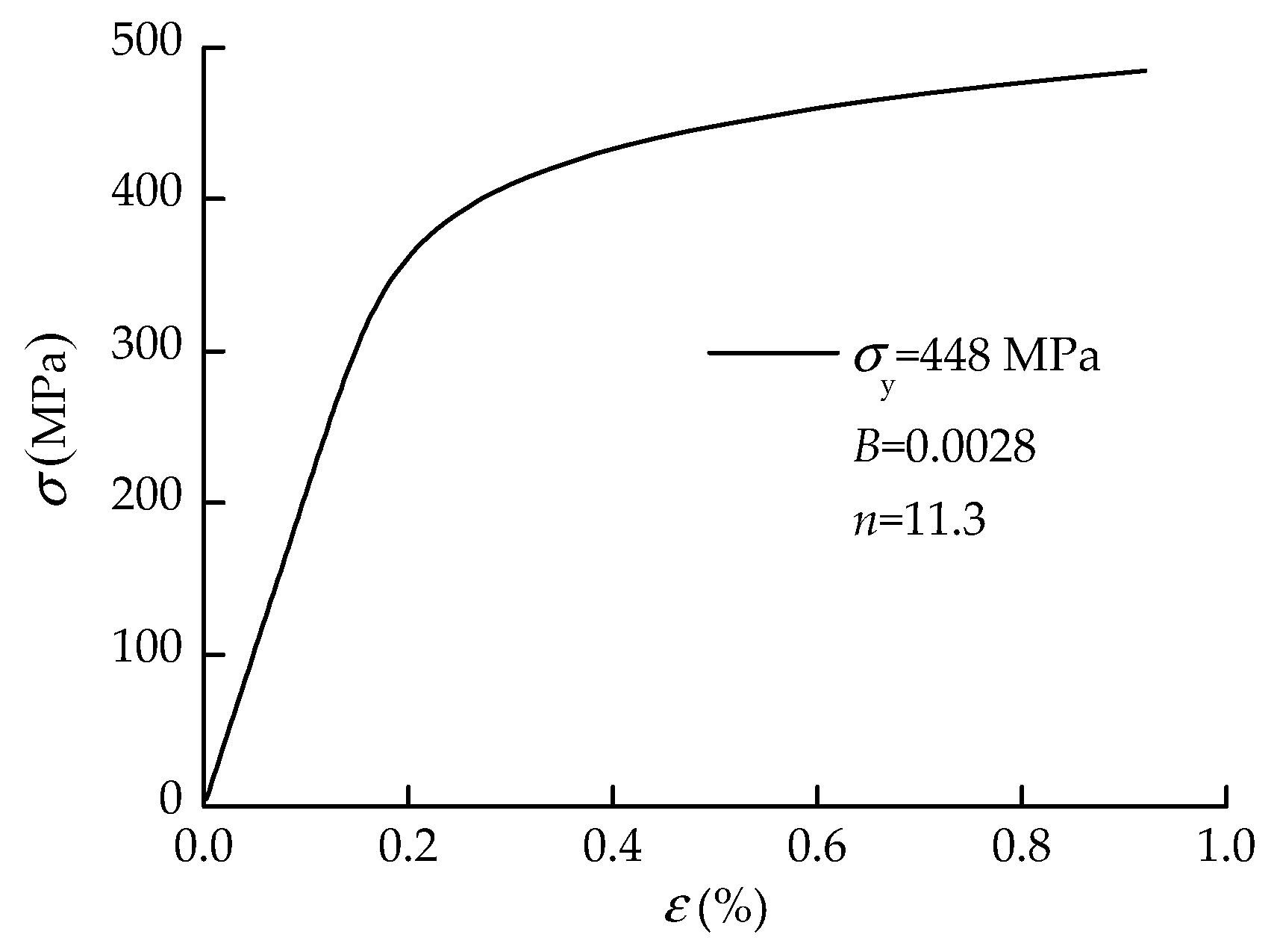
  27. Ramberg, W.; Osgood, W.R. Description of Stress-Strain Curves by Three Parameters; Technical Note, No. 902; National Advisory Committee for Aeronautics (NACA): Washington, DC, USA, 1943. [Google Scholar]
  28. Wang, F.C.; Luo, Y.; Xie, Y.; Li, B.; Li, J.N. Practical and theoretical assessments of subsea installation capacity for HYSY 201 laybarge according to recent project performances in South China Sea. In Proceedings of the Annual Offshore Technology Conference, Houston, TX, USA, 5–8 May 2014; pp. 2696–2704. [Google Scholar]
  29. Randolph, M.F.; Quiggin, P. Non-linear hysteretic seabed model for catenary pipeline contact. In Proceedings of the 28th International Conference on Ocean, Honolulu, HI, USA, 31 May–5 June 2009. [Google Scholar]
  30. Gong, S.F.; Xu, P. Influences of pipe–soil interaction on dynamic behaviour of deepwater S-lay pipeline under random sea states. Ships Offshore Struct. 2017, 12, 370–387. [Google Scholar] [CrossRef]
  31. Ai, S.M.; Sun, L.P.; Tao, L.B.; Yim, C.S. Modeling and simulation of deepwater pipeline S-lay with coupled dynamic positioning. J. Offshore Mech. Arct. Eng. 2018, 140, 051704. [Google Scholar] [CrossRef]
  32. Slunyaev, A.; Pelinovsky, E.; Sergeeva, A.; Chabchoub, A.; Hoffmann, N.; Onorato, M.; Akhmediev, N. Super-rogue Waves in Simulations Based on Weakly Nonlinear and Fully Nonlinear Hydrodynamic Equations. Phys. Rev. E Stat. Nonlinear Soft Matter Phys. 2013, 88, 012909. [Google Scholar] [CrossRef] [Green Version]
  33. Lu, W.Y.; Yang, J.M.; Fu, S.X. Numerical Study of the Generation and Evolution of Breather-type Rogue Waves. Ships Offshore Struct. 2017, 12, 66–76. [Google Scholar] [CrossRef]
  34. Morison, J.R.; O’Brien, M.D.; Johnson, J.W.; Schaaf, S.A. The force exerted by surface waves on piles. J. Pet. Technol. 1950, 2, 149–154. [Google Scholar] [CrossRef]
  35. White, D.J.; Cheuk, C.Y. Modelling the soil resistance on seabed pipelines during large cycles of lateral movement. Mar. Struct. 2008, 21, 59–79. [Google Scholar] [CrossRef]
Figure 1. Deepwater pipeline installation by the S-lay method under exposure to freak waves.
Jmse 08 00119 g001
Figure 2. Node and line segment model of the S-lay pipeline.
Jmse 08 00119 g002
Figure 3. Schematic diagram of the deepwater S-lay stinger: (a) Pipe–roller interaction; (b) articulated stinger of the Hai Yang Shi You (HYSY) 201 vessel.
Jmse 08 00119 g003
Figure 4. Non-linear hysteretic seabed soil model [29].
Jmse 08 00119 g004
Figure 5. Modified Coulomb friction model.
Jmse 08 00119 g005
Figure 6. Motion response spectra of the HYSY 201 pipelay vessel at the stinger base.
Jmse 08 00119 g006aJmse 08 00119 g006b
Figure 7. JONSWAP spectrum for Hs = 2.0 m.
Jmse 08 00119 g007
Figure 8. Time history trains of the freak wave.
Jmse 08 00119 g008
Figure 9. Time history trains of freak waves under different input conditions: (a) energy ratio coefficient; (b) focusing position; (c) phase range; (d) wave peak value.
Jmse 08 00119 g009
Figure 10. Variation of the maximum freak wave height with different input conditions: (a) energy ratio coefficient; (b) focusing position; (c) phase range; (d) wave peak value.
Jmse 08 00119 g010
Figure 11. Stress–strain curve for the Ramberg–Osgood model.
Jmse 08 00119 g011
Figure 12. Non-linear hysteretic moment–curvature relationship.
Jmse 08 00119 g012
Figure 13. Current speed distribution with various water depths.
Jmse 08 00119 g013
Figure 14. Time history responses of pipelay vessel motions under freak waves.
Jmse 08 00119 g014
Figure 15. Dynamic responses of the S-laying pipeline under various freak wave energy ratio coefficients: (a) tension; (b) bending moment; (c) stress; (d) strain; (e) pipeline embedment; (f) seabed resistance.
Jmse 08 00119 g015
Figure 16. Dynamic responses of the S-laying pipeline under various freak wave focused positions: (a) tension; (b) bending moment; (c) stress; (d) strain; (e) pipeline embedment; (f) seabed resistance.
Jmse 08 00119 g016
Figure 17. Dynamic responses of the S-laying pipeline under various freak wave phase ranges: (a) tension; (b) bending moment; (c) stress; (d) strain; (e) pipeline embedment; (f) seabed resistance.
Jmse 08 00119 g017
Figure 18. Dynamic responses of the S-laying pipeline under various freak wave peak values: (a) tension; (b) bending moment; (c) stress; (d) strain; (e) pipeline embedment; (f) seabed resistance.
Jmse 08 00119 g018aJmse 08 00119 g018b
Figure 19. Effect of freak wave conditions on dynamic amplification factors of pipeline behaviors and seabed resistance: (a) energy ratio coefficients; (b) focused position; (c) phase range; (d) peak value.
Jmse 08 00119 g019
Table 1. Laying pipeline parameters.
D (mm)tp (mm)ρp (kg/m3)E (MPa)vσy (MPa)tc (mm)ρc (kg/m3)wa (N/m)ws (N/m)
323.923.878502.07 × 1050.34483.09501754.9917.2
Table 2. Seabed soil model parameters.
Su0 (kPa)Sug (kPa/m)ρsoil (t/m3)abKmaxfsucλsucλrepfbμks (kN/m3)
1.51.51.56.00.252000.61.00.31.50.5533.3

