Bubble Sweep-Down of Research Vessels Based on the Coupled Eulerian-Lagrangian Method

Abstract

To explore the reason for the bubble sweep-down phenomenon of research vessels and its effect on the position of the stern sonar of a research vessel, the use of a fairing was investigated as a defoaming appendage. The separation vortex turbulence model was selected for simulation, and the coupled Eulerian-Lagrangian method was adopted to study the characteristics of the bubble sweep-down motion, captured using a discrete element model. The interaction between the bubbles, water, air, and hull was defined via a multiphase interaction method. The bubble point position and bubble layer were calculated separately. The spatial movement characteristics of the bubbles were extracted from bubble trajectories. It was demonstrated that the bubble sweep-down phenomenon is closely related to the distribution of the bow pressure field and that the bubble motion characteristics is related to the speed and initial bubble position. When the initial bubble position is between the water surface and the ship bottom, the impact on the middle of the ship bottom is greater and increases further with increasing speed. A deflector forces the bubbles to both sides through physical shielding, strengthening the local vortex structure and keeping bubbles away from the middle of the ship bottom.

1. Introduction

Exploring and understanding the ocean are prerequisites for the development of marine resources and the protection of the marine ecological environment. The marine research vessel is a type of ship extremely suitable for this. The research vessel is dedicated to scientific investigations of the sea, with the purpose of obtaining comprehensive marine geology, biology, and ecology survey information of the atmosphere, for example. As the “eye” of the research vessel, the sonar equipment, specifically its performance, plays a vital role in the accuracy of the research vessel’s detection results.

Karafiath [1] analyzed the occurrence of the phenomenon of bubble sweep-down and believed that, under actual sea conditions, owing to the strong fluidity of seawater, strong sea breeze, and the effects of wave breaking and rainwater impact, the seawater near the water surface has a certain air content, within a certain water depth range. A layer of suspended bubbles is formed in this water layer.

Deane and Stokes [2] measured the bubble size distribution in breaking waves in the laboratory and on the high seas, provided a quantitative description of the bubble formation mechanism in the laboratory, and analyzed the dependence of scale on bubble generation and propagation and the mechanism of breaking wave conditions. Thorpe [3] described the fact that small bubbles with a radius of less than 1 mm are stabilized by surface tension, whereas bubbles with a larger radius are broken by the shear stress in the turbulent motion caused by the collapse event. Smaller bubbles rise very slowly; hence, they persist in the water column and flow at greater depths. When the research vessel sails in this bubble layer, the bubbles move along the hull surface owing to hull wakes. Moving down to the bottom of the ship, the phenomenon of bubble downward scanning occurs, which affects the performance of the sonar at the stern position and affects the detection function of the research vessel. Sebastian and Caruthers [4] recorded the impact on the operation of a multibeam sonar.

For some ship types, an excellent inlet design can eliminate the down-sweep phenomenon of bubbles, but the phenomenon still appears after the speed increases. Rolland [5] shows that direct installation of a defoaming attachment inevitably brings a certain increase in resistance, sometimes even up to 20%. Therefore, it is a better direction to first study the bubble motion characteristics of the transducer surface.

The current research on ship performance widely uses a ship model pool, and the scale effect is unavoidable. It is difficult to form a uniform microbubble layer in the water. It can only be supplemented by a bubble generator to generate bubbles in real time. To make matters worse, large physical pools are often left for a long time, resulting in pools containing far less air, so that bubbles dissolve in water more quickly than under actual sea conditions. Therefore, this study combines research on computational fluid dynamics (CFD) methods, which was conducted to verify, e.g., conventional resistance research, and single or limited location bubble generation research.

Delacroix [6] quantified the backscattered signal on the bubble cloud image with an echo sounder, and studied the influence of wind speed under navigation conditions on the characteristics of the bubble sweep-down. Mallat [7] used the particle image velocimetry (PIV) test method, using the bow longitudinal section and in the form of streamline, to study the 3D characteristics of the sweep-down of the bubble.

Many people, including Han [8], have used CFD for many years for hull shape optimization. Delacroix used it for a characteristic study of bubble sweep-down and Palaniappan and Subramanian [9] worked out the hydrodynamic design for bubble sweep-down.

In order to make up for the deficiencies of the bubble experiment in the pool, this study used the Eulerian-Lagrangian method to model the bubbles, as described in Section 2, and the CFD method was adopted to calculate the bubble point and bubble layer. By ignoring the dissolution and breaking of bubbles, the phenomenon of bubble sweep-down was studied. In Section 3, the accuracy of the CFD calculation method is verified through the resistance and single-bubble point towing tank test. In Section 4, we show more comprehensive calculation results, including further calculation and extraction results of bubble characteristics and flow field details such as velocity field.

2. Numerical Method

2.1. Governing Equations

Energy exchange is not involved in the research, and the continuity equation and momentum equation are, respectively, as follows:

$$\frac{\partial }{\partial t}\left(a_q{\rho }_q\right)+\nabla \cdot \left(a_q{\rho }_q{\mathit{v}}_q\right)=0$$

(1)

$$\frac{\partial }{\partial t}\left(\rho \mathit{v}\right)+\left(\rho \mathit{v}\mathit{v}\right)=-\nabla p+\nabla \cdot \left[\mu \left(\nabla \mathit{v}+\nabla {\mathit{v}}^T\right)\right]+\rho g+F$$

(2)

where $a_q$ is the volume fraction of phase $q$, ${\rho }_q$ is the density of phase $q$, $\rho$ is the mixed phase density, ${\mathit{v}}_q$ is the velocity of phase $q$, $\mu$ is the sum of turbulent viscosity and molecular mixing viscosity, $g$ is the acceleration, and $F$ is the external force.

2.2. Turbulence Model and Coupled Eulerian-Lagrangian Method

In the research of microbubble scale, it is considered that the bubble and water are both interacting and represent two relatively independent phases. The bubble phase is located in the water phase but is not soluble in water. When the volume fraction is used to express the volume fraction of the phase, the volume fraction function of the two phases of bubbles and water is continuous in time and space and the sum is 1. The volume of fluid (VOF) method is used to track the interface between the two phases of water and air, and the bubbles ejected from the bow of the ship are used as discrete bubble-phase particles distributed in the continuous fluid domain, and the motion model of the bubble particles is established by the discrete element method (DEM) method. In the study, the bubble diameter was set to 1 mm, and the bubble spacing was 16.8 mm. Therefore, the interaction between the bubble particles is relatively weak, and the influence on the continuous fluid domain can be ignored.

Maxwell [10] used the DEM model to study the interaction force between bubbles and particles and the sliding of particles. Bérard [11] summarized the progress of a CFD-DEM calculation of solid-liquid coupling in chemical engineering. Based on the coupled Eulerian-Lagrangian method, Xinhong Li [12] solved the trajectory of the discrete-phase bubble particles, so that the force is balanced during the movement as follows:

$$\frac{d{u}_p}{dt}=F_d\left(u-u_p\right)+\frac{g\left({\rho }_p-\rho \right)}{{\rho }_p}+F$$

(3)

where $u$ is the towing speed of the ship, $u_p$ is the bubble particle velocity, $F_d$ is the drag force, measured by experiment, $\rho$ is the continuous phase density, and ${\rho }_q$ is the bubble particle density.

The sweep-down of bubbles involves capturing motion near the wall of the hull. The shear stress transmission (SST) k-omega detached eddy simulation (DES) turbulence model is used for simulation to close the equation.

DES is a hybrid modeling method that uses time-averaged Reynolds-averaged Navier-Stokes (RANS) to solve near the wall boundary layer, while the turbulence is away from the wall. The area is solved by transient large eddy simulation (LES), which balances calculation accuracy and calculation cost. Zhang and Ahmadi [13] used the Eulerian-Lagrangian calculation model to simulate gas-liquid-solid three-phase flow. Watson [14] used a delayed separation vortex simulation to calculate the unsteady flow of the ship hull. Home and Lightstone [15] used DES-SST to study the flow of interstitial vortices. Jee and Shariff [16] proposed the v2-f DES model and calculated the cylindrical flow around and the turbulence phenomena. Although DES reduces the requirements for computing grids compared to LES, the requirements for grid quality are still higher.

The SST model was used to simulate the inverse pressure gradient near the wall. With respect to the unsteady flow, the finite volume method was used to solve the problem, and the coupling solver of VOF and DEM was used.

2.3. Numerical Scheme in CFD

CFD calculation software STAR-CCM+ was used for numerical calculation, and the grid scheme was designed according to the above calculation model method. The geometry of the hull and the boundary conditions established in CFD are shown in Figure 1.

The main parameters of the hull are shown in

Table 1. Main parameters of the research vessel.

Item	Symbol	Real Ship	Model	Unit
Waterline length	LWL	90.2	3.608	m
Breadth	B	16.8	0.672	m
Fore draft	TF	5	0.2	m
Aft draft	TA	5	0.2	m
Displaced volume	▽	3844.6	0.2461	m3
Wet surface area	S0	1663	2.661	m2
Longitudinal center of buoyancy	LCB	41.008	1.64	m
Block coefficient	CB	0.5074
Scale ratio	λ	1	25

.

Since the hull is symmetrical, calculations were performed on the half hull to save computing resources. Considering that a considerable part of the bubbles were entrapped by the bow vortex to the bottom of the ship, additional structured grid discretization of the bow grid and free surface was required in the CFD calculation, as shown in Figure 2.

To simulate the navigation state under natural conditions and facilitate the analysis of the movement characteristics of a single bubble, two schemes were set up for calculation. The structured grid discretization of the wall is shown in Figure 3b. The final number of grid cells generated was 11.84 million.

The following two schemes were used to calculate the movement of bubbles:

Scheme 1. For natural conditions, the bubbles in the water exist in the form of a suspended relatively stable bubble layer; hence, it is necessary to calculate the movement characteristics of the bubble layer under this condition. To make the bubble development more complete, we set the bubble layer in the bow of the ship (0.042 LWL in the front) and can observe that 40 bubble points in the vertical direction cover a certain draft range and 80 bubble points in the width direction of the ship are larger than the width of the ship. The relative position of the bow and the bubble layer is shown in Figure 3a.

Scheme 2. The position of the bubble point is the same as the test, as shown in Figure 3b.

As shown in Figure 4, the Y+ value of the final generated grid scheme is within 1.

According to the International Towing Tank Conference (ITTC) ’s convergence judgment criterion, when a CFD calculation is used, three sets of grid schemes with different grid sizes are obtained by changing the basic size of the grid according to the fixed fineness ratio $\sqrt{2}$. The uncertainty analysis of the resistance calculation results of the scheme is then carried out.

According to the principle that the convective Courant number is less than 1, the time step of non-steady state calculation is set to 0.001. The grid schemes compared are shown in the

Table 2. Number of grids and simulated resistance.

Grid Scheme	Base Size (M)	Number of Grids (Million)	Simulated Drag Coefficient ×10³	Test Resistance Coefficient ×10³
1	0.1	6.8	4.745	4.827
2	0.071	9.7	4.782
3	0.05	11.8	4.790

.

According to the data in Table 2, in the process of gradually increasing the number of grids from scheme 1 to scheme 3, we can judge according to the grid convergence rate as follows:

$$\begin{array}{l}{\epsilon }_{G21}=R_2-R_1\\ {\epsilon }_{G32}=R_3-R_2\end{array}$$

(4)

$$R_G=\frac{{\epsilon }_{G32}}{{\epsilon }_{G21}}=0.22$$

(5)

The grid convergence rate, $R_G$, is a positive number less than 1, which conforms to the ITTC’s grid convergence criteria. It shows that the calculation scheme is convergent. The smaller the value, the faster the convergence speed. The uncertainty is further verified according to the ITTC standard. The results for the correlation coefficient of the uncertainty analysis are shown in

Table 3. Uncertainty verification of resistance.

Ctm1	RG	PG	CG	UG	${\delta }_G^{*}$	${U_G}_c$
4.790	0.216	1.531	0.70	0.0114	0.010	0.003

.

The order estimate $P_G$ is greater than 1, indicating that the resistance calculation accuracy is high. From the correction factor $C_G$ value near 1, it can be concluded that the resistance calculation result is near the asymptotic value after convergence. The error ${\delta }_G{}^{*}$ with correction factor and the uncertainty $U_{Gc}$ of the correction value can then be estimated.

At the same time, in the calculation of the bubble, in order to reflect the state of the ship passing the bubble at a constant speed and the stability of the calculation, the conventional resistance is calculated first, and the bubble jet is activated after the resistance calculation is stable. It takes at least 20 s of physical time for resistance calculation to stabilize, and at least 40 s for bubble calculation.

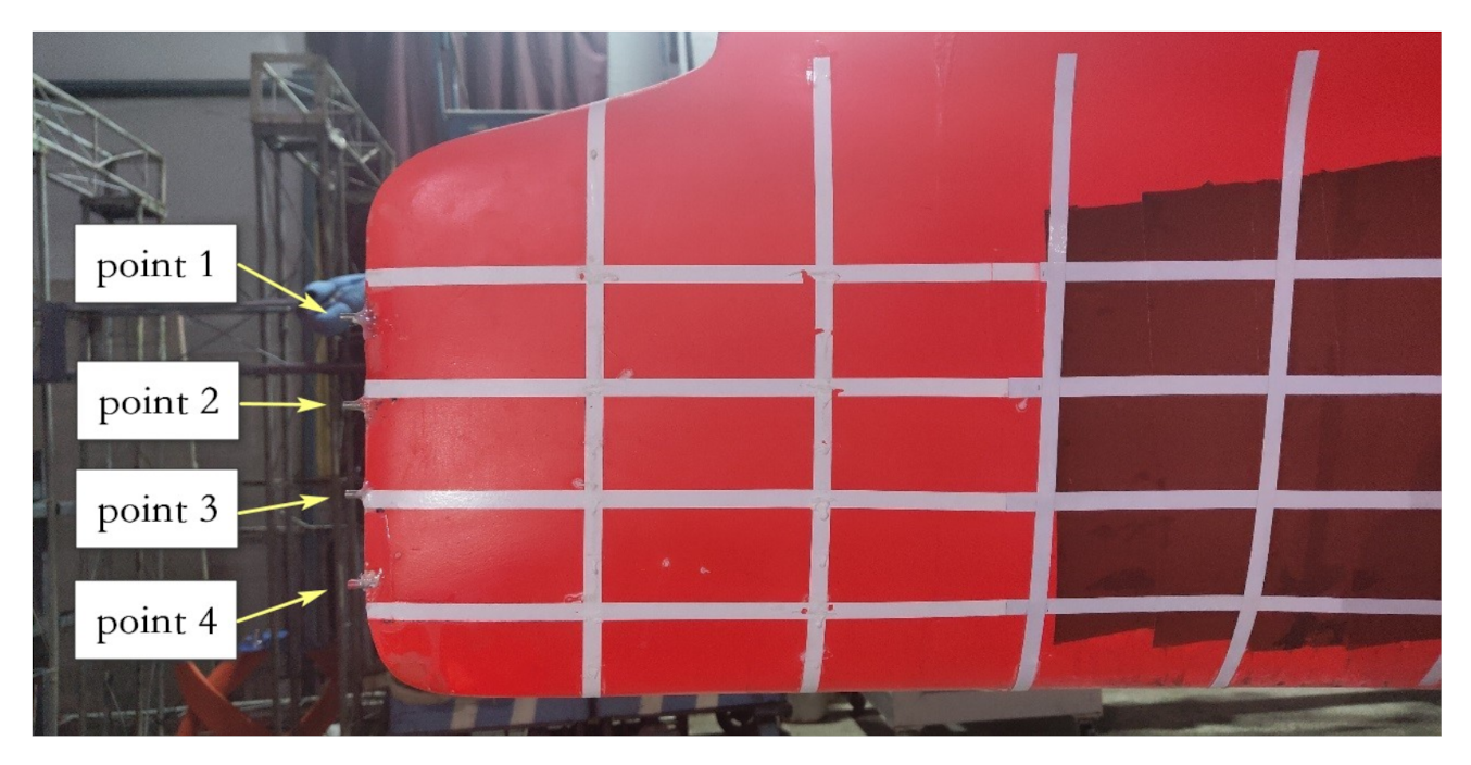
3. Experimental Method

The resistance test adopts the method of fixing the posture of the model, and the test is completed in the towing tank of the ship model of Harbin Engineering University, Harbin, China. The static state of the ship model after installation is shown in Figure 5.

For large towing pools, the air content is usually much lower than for real sea conditions. It is extremely difficult to generate a suspended bubble layer similar to real sea conditions. Therefore, a bubble generator is used to generate bubbles at a vertical spacing of 0.04 m below the bow water surface. The four vent holes are connected to the bubble generator to observe the position of the individual bubble generation point. The opening position is shown in Figure 6.

The experiment uses the PIV method to obtain the spatial movement information of the bubbles by using the white stripe positioning on the surface and laser irradiation.

As the main diameter of the bubble sweep-down is 500–1000 μm, it is necessary to generate 20–40 μm bubbles. The bubble generator used in the test produces bubbles in the range of 10–50 μm, which meets the test requirements. The working conditions of the resistance test are shown in

Table 4. Test conditions.

Actual Ship Speed Vs (Kn)	Froude Number Fr	Model Speed Vm (m/s)	Trim Angle (°)	Wave
12	0.225	1.234	0	Static water
16	0.277	1.646	0	Static water

, and numerical calculations were carried out under the same working conditions.

A sweep-down test of air bubbles was carried out with a working speed of 1.234 m/s in a pool.

4. Results and Analysis

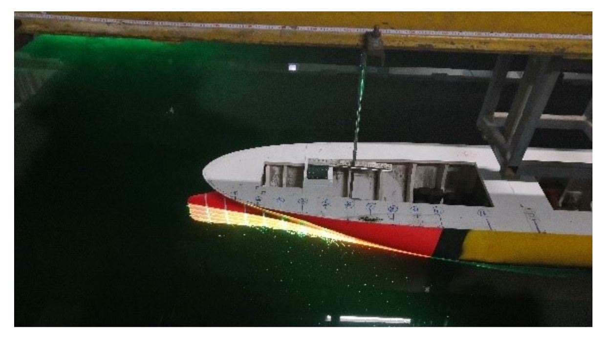
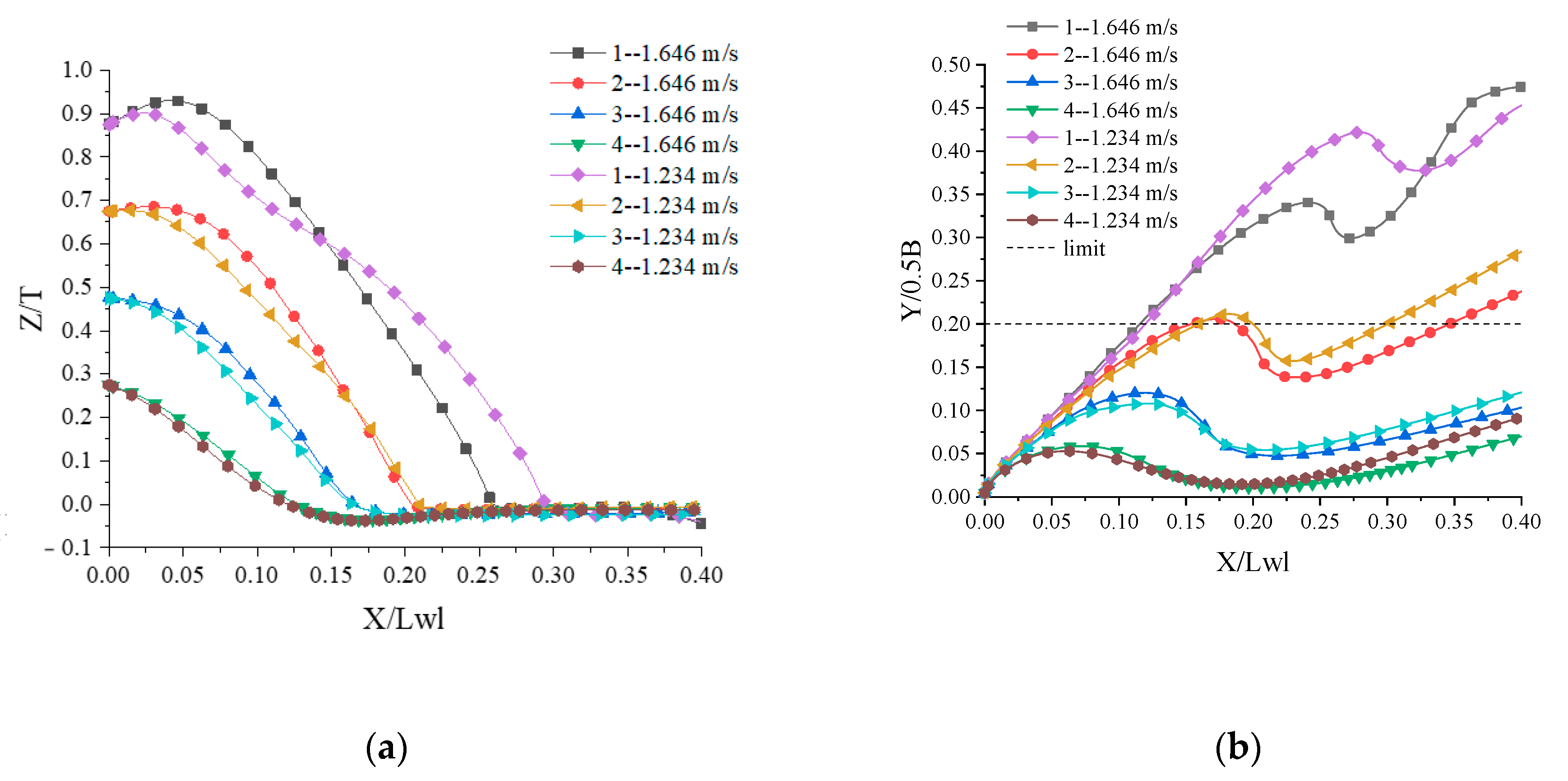
4.1. Spatial Movement Characteristics of Bubbles Under Sweeping

The results of the resistance test were verified. The test results of bubble motion at a multibeam operating speed of 1.234 m/s are shown in Figure 7.

In Figure 7, the trajectory of the bubbles is highlighted and extracted in yellow by the bubble point. Figure 7e is a cross-sectional bubble cloud diagram obtained by PIV. The space movement position of the bubble cluster center is obtained by the white grid line in Figure 7 and this cloud image. The base point is located in front of the bow of the ship, with the length of the ship as the X-axis and the stern direction as the positive direction. The trajectories in the longitudinal plane (X-Z direction) and the horizontal plane (X-Y direction) result in line graphs, expressed in dimensionless form, by dividing by T and L_wl, respectively. Here, T represents the average draft.

In the test, the size of the bubbles is extremely small because of the scale, which makes them difficult to observe. It is speculated that the bubbles generated by the bubble generator in the experiment have different sizes, and the density of the bubbles generated in the experiment is larger, resulting in stronger interactions such as fusion. Therefore, the lift force of the bubble is increased to a certain extent, and the density of the bubble in the actual sea state is relatively low, and the numerical results are considered to be relatively consistent. Although the bubbles sweep down near the bow of the ship, they dissolve in the water quickly. Therefore, it is necessary to carry out CFD calculations and tests at multibeam working speed. The trajectory comparison between the experiment test results and the CFD calculation results is shown in Figure 8.

It can be seen that the bubble motion trajectories of the four bubble generation points are close, but the bubble sweep-down calculated by CFD at point 2 is faster. According to Figure 7, the sweep-down trend of bubble points 3 and 4 is obvious, and bubble point 1 is the most affected by wave making. Bubble point 2 is in the area where the wave making is obviously weakened, but there is still a sweep-down trend under the dual effects of wave making and relatively steady flow. However, the relatively deeper dip of bubble points 3 and 4 is not as obvious here.

Combining the test and calculation results, the CFD method is feasible to calculate bubble motion characteristics. The calculation of bubble motion and flow field details was carried out. The calculation results of bubble layer and bubble point under multibeam working speed and research vessel design speed are shown in Figure 9 and Figure 10.

It can be seen that, when the research vessel is sailing, the bubbles located in the front of the hull sweep under the surface of the hull to the bottom of the ship, causing a large number of bubbles to accumulate at the bottom of the ship. It is particularly obvious at the higher of the calculated speeds. This has a significant influence on the position of the sonar at the stern of the ship. From the calculation of the bubble layer in Figure 9, it can also be seen that, when sailing under natural conditions, in addition to the bubbles that produce the sweep-down phenomenon, a large number of bubbles move with the hull. Regular analysis becomes difficult; hence, the fixed bubble point positions are calculated.

In the comparison between the bubble point in Figure 10 and the calculation result of the bubble layer setting in Figure 9, the first bubble layer tilts down with the water surface, which has the characteristics of sweep-down. A large number of bubbles gather near the center line of the bottom surface of the ship and the bubble layer trajectory covers the trajectory of the bubble point. However, when the bubble point is set at 1.234 m/s, the sweep-down trend of the bubble point is more obvious than that of the bubble layer. It is speculated that the bubble layer has a higher density, relatively low speed, and relatively turbulent wave making, which causes more frequent interactions between the bubbles. Under actual sea conditions, as the size of the bubble becomes larger but the relative density becomes smaller, the effect of the bubbles on the surface of the hull is relatively weakened. From the image results, the above calculation of individual bubble points can better reflect the movement of the bubble layer state. The results at different speeds are shown in Figure 11.

Extracting the bubble space movement trajectory, the bubble X-Z spatial movement characteristics (Figure 11a) are obtained. The bubble initially floats up for a period of time, and then it moves down to the bottom of the ship, and finally moves to the rear of the ship under the bottom of the ship. The starting position of this final stage can be set as the down-sweep point. The lower the position of the bubble, the closer to the bow of the ship when it sweeps down to the bottom, and the lower the speed (absolute value of the tangential slope of the curve) during the sweep-down. With increasing speed, both the initial floating process of the bubbles and the sweep-down part are enhanced. The bubble at the same position sweeps down to the bottom of the boat and moves toward the bow, and the velocity at which the bubble sweeps down increases. According to the bubble movement trajectory curve in the X-Z direction, the lower sweep position of the bubble movement can be divided into the following two movement processes: before and after the lower sweep. For the speed of 1.234 m/s, the lower sweep point is 0.27 L and, for 1.646 m/s, it is 0.26 L.

The bubble movement curve in the width direction of the ship is used to analyze the influence of bubble movement on the position of the center line of the hull, and then to measure its influence on the sonar at the stern, as shown in Figure 11b. The bubble movement curve in the X-Y direction has two obvious curvature optimum points, that is, the peak appears first and then the valley. Combined with the hull model, the peak is the position that sweeps down to the outside of the bottom of the ship. The valley is the position closest to the mid-longitudinal section of the hull where the bubbles can continue to move from the outside of the bottom. The movement between peaks and valleys is the sweep-down process, and the sweep point of the bubble is also located in this process. The lower the initial bubble position, the closer the valley position after the sweep-down is to the middle of the ship. As the speed increases, this position moves toward the bow. After that, the bubble movement gradually moves away from the midship position, but it still has an impact on the position of the sonar at the stern. The dotted line in Figure 11b represents the safety limit line. The bubbles at positions 3 and 4 have a great impact on the multibeam.

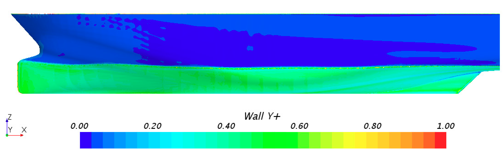
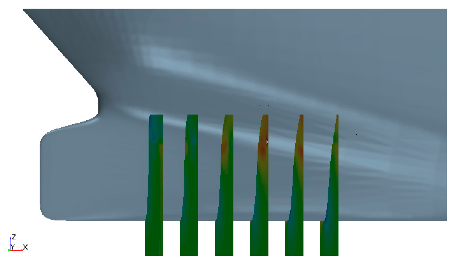
4.2. Flow Around the Bow

The next step is to calculate the distribution of the pressure field near the bow and analyze the relationship between the bubble sweep-down phenomenon and the pressure field.

The pressure coefficient is defined by $C_p=\left(P-\rho \mathrm{gh}\right)/0.5\rho V_0{}^2$, where $V_0$ represents the speed, and we can obtain the dimensionless pressure difference relative to the hydrostatic pressure. The streamline set by the bubble point is represented by a gray-white line. The calculation result is shown in Figure 12.

From the surface pressure distribution of the hull at different speeds in Figure 12, it can be concluded that the bow pressure is relatively high, a maximum value appears at the peak of the bow wave surface uplift, and the pressure gradually decreases toward the back of the ship and the bottom of the ship. Therefore, it is easy to force the microbubbles in the water to move during the navigation. The bubbles migrate from the high-pressure position to the low-pressure position under the action of the pressure difference. The bottom of the ship has a minimum pressure value, and the bubbles continue to the middle of the bottom of the ship owing to the inertial movement, and then move backward with the ship sailing. Because the shape of the bow of the research vessel in this study is relatively flat, the bubbles migrate to the bottom of the ship under the dual effects of the bow wake and the pressure difference, resulting in the phenomenon of bubble sweep-down. The pressure distribution changes with speed. At the higher speeds, the pressure coefficient of the side and bottom of the ship is smaller than that at lower speeds; hence, bubble sweep-down is more likely to occur at high speeds.

The velocity field distribution of multiple cross-sections at the bow of the hull was calculated, where the zero point of the cross-section corresponds to the foremost end of the deck, and the direction to the stern is the positive x direction and the vertical upward direction is the positive z direction. The cross-sectional positions 0.45, 0.55, 0.65, 0.75, and 0.85 m are shown in Figure 13.

Through calculation, the vertical velocity distribution on the cross-section is obtained, and the vertical velocity is expressed in dimensionless $V_Z/V_0$, where $V_Z$ is the vertical velocity component, $V_0=V_m$, which is the towing speed of the ship model. Furthermore, the position of the bubble and the position of the free water surface (the horizontal black line) on the cross-section are marked, as shown in Figure 14 and Figure 15.

According to the vertical dimensionless velocity distribution of multiple cross-sections in Figure 14 and Figure 15, it can be concluded that the vertical velocity component near the hull wall below the water surface is only upwards in the part closest to the water surface. This upward velocity core area moves back with the section position at 1.234 m/s, first close to the hull and then away from the hull, but keeps away from the hull at 1.646 m/s. This is related to the influence of the hull’s wave making. The vertical downward velocity component near the wall gradually increases. The downward velocity core area formed increases with the increase in speed, reaches the maximum value near the bottom of the ship, and then gradually decreases. The range of motion is in this wall area. According to the change of the bubble position, it can be seen that the trajectory of the bubble before it moves to the bottom of the ship is near the vertical downward velocity core area. This provides a certain amount for the sweep-down of the bubble. When the bubble moves to the bottom of the ship, a vertical upward velocity component is generated, so that the bubble moves upward to the bottom of the ship while moving toward the stern. This is also one of the reasons why the sweep-down of the bubble affects the position of the stern sonar.

4.3. Shroud

A diversion cover was used as a defoaming appendage, and the principle of action was calculated and analyzed. The geometric shape and the installation position of the diversion cover are shown in Figure 16. Some parameters of the shroud are shown in

Table 5. Some parameters of the shroud.

Item	Symbol	Model	Unit
Displaced volume	▽	0.0002	m3
Wet surface area	S	0.0416	m2
Installed surface area	S	0.0295	m2

.

According to the shroud’s parameters, the installation of the deflector has minimal impact on the parameters of the bare hull. Among them, the displacement is increased by 0.08%, and the wet surface area is increased by 0.4%. The draft is increased by less than 0.22 mm, and its impact is almost negligible. The comparison of the vorticity distribution at the bottom of the ship is shown in the Figure 17.

According to the calculation results in Figure 17, the structure of the vortex system at the bottom of the ship is relatively simple. There are two parts of the vortex system distributed on the side of the ship and the bottom of the bow. The deflector effect of the vortex system on the ship side is minimal, but the ship bottom vortex structure is dispersed, changing the vortex structure in the middle of the bottom of the ship. First, the position of the deflector is located at the position of the vortex structure on the first center line of the hull, which eliminates or greatly reduces the effect of this vortex structure in bringing bubbles into the ship. The installation of the diversion cover adds a vortex structure away from the ship, which makes the bubbles move outward along the edge of the diversion cover from both the physical shielding and the vortex structure guidance. Based on this, the diversion cover has a certain defoaming performance.

The changes in the total resistance coefficient and the remaining resistance coefficient are shown in Figure 18. The influence of the dome on the resistance performance is mainly reflected in the increase in the residual resistance of the hull within a certain low speed range, and the maximum increase in the total resistance can reach 5.1%. However, the influence gradually decreases as the speed increases. For the two calculated speeds, the drag increase in the dome is extremely small.

Based on the comparison of the defoaming effect before and after the installation of the diversion cover, shown in Figure 17, and the resistance increase, shown in Figure 18, the diversion cover can produce a small increase in resistance and at the same time reduce the effect of bubble sweep-down on the stern.

5. Conclusions

The results of the research on the phenomenon of sweep-down of bubbles in research vessels provide the following conclusions.

1)

It is feasible to use the Eulerian-Lagrangian method to calculate the bubble sweep-down phenomenon.

2)

The phenomenon of bubble sweep-down is related to the shape of the bow of the ship and the distribution of the pressure field. The pressure difference caused by the decrease in the hull surface pressure with the increase in water depth and the vertical downward velocity component near the wall forces the bubbles to sweep down.

3)

The movement characteristics of the bubble sweep-down space are related to the initial position and speed of the bubble. When the bow is closer to the bottom of the ship, the sweeping position of the bubble is closer to the bow, and the position after the bottom of the ship is closer to the center line of the bottom of the ship. Therefore, the influence on the position of the stern sonar is greater, and the degree of this influence increases with the increase in speed.

4)

After the bubble moves through the sweep-down point, it moves to the center line of the bottom of the ship to strengthen the influence on the sonar position. From the perspective of hydrodynamics, the installation of the diversion cover plays the role of physical shielding and strengthens the guidance of the lateral vortex system, so that the bubbles move to the side of the ship with the vortex to achieve the purpose of defoaming.

5)

The installation of the shroud produces a certain increase in resistance while achieving a certain defoaming effect, which is especially obvious at low speeds but is already extremely small at working speeds. This occurs because viscous resistance dominates at lower speeds, whereas pressure resistance is more important at higher speeds.

The spatial motion of the bubble sweep-down and the fine characteristics of the partial flow field were studied and the above results were obtained. The research results have some reference value for the law of bubble sweep-down of research vessels and for the reduction of its influence on sonar equipment spatially. However, the work was carried out only from the hydrodynamic point of view, without considering the noise characteristics under the actual sonar work. In addition, the dissolution and breakage of bubbles were ignored. This method is beneficial to the study of bubble movement, but the adverse effect on the study of noise cannot be ignored. The follow-up work will study the influence of the bubble sweep-down phenomenon based on the noise characteristics of sonar work, such as frequency.

References

1. Karafiath, G.; Hotaling, J.M.; Meehan, J.M. Fisheries Research Vessel hydrodynamic design minimizing bubble sweep-down. In Proceedings of the Oceans 2001 MTS/IEEE Conference and Exhibition, Washington, DC, USA, 5–8 November 2001; Volume 2, pp. 1212–1223. [Google Scholar]
2. Deane, G.B.; Stokes, M.D. Scale dependence of bubble creation mechanisms in breaking waves. Nat. Cell Biol. 2002, 418, 839–844. [Google Scholar] [CrossRef] [PubMed]
3. Thorpe, S.A. The Turbulent Ocean; Cambridge University Press: Cambridge, UK, 2005; pp. 240–243. [Google Scholar]
4. Sebastian, S.M.; Caruthers, J.W. Effects of naturally occurring bubbles on multibeam sonar operations. In Proceedings of the Oceans 2001 MTS/IEEE Conference and Exhibition, Washington, DC, USA, 5–8 November 2001; Volume 2, pp. 1241–1247. [Google Scholar]
5. Rolland, D.; Clark, P. Reducing bubble sweep-down effects on research vessels. In Proceedings of the Oceans 2001 MTS/IEEE Conference and Exhibition, Washington, DC, USA, 5–8 November 2001; pp. 1–7. [Google Scholar]
6. Delacroix, S.; Germain, G.; Berger, L.; Billard, J.-Y. Bubble sweep-down occurrence characterization on Research Vessels. Ocean. Eng. 2016, 111, 34–42. [Google Scholar] [CrossRef] [Green Version]
7. Mallat, B.; Germain, G.; Billard, J.-Y.; Gaurier, B. A 3D study of the bubble sweep-down phenomenon around a 1/30 scale ship model. Europ. J. Mech. 2018, 72, 471–484. [Google Scholar] [CrossRef] [Green Version]
8. Han, S.; Lee, Y.-S.; Choi, Y.B. Hydrodynamic hull form optimization using parametric models. J. Mar. Sci. Technol. 2012, 17, 1–17. [Google Scholar] [CrossRef] [Green Version]
9. Palaniappan, M.; Subramanian, V.A. Hydrodynamic design for mitigation of bubble sweep down in sonar mounted research vessels. Int. Shipbuild. Prog. 2017, 64, 101–126. [Google Scholar] [CrossRef]
10. Maxwell, R.; Ata, S.; Wanless, E.; Moreno-Atanasio, R. Computer simulations of particle–bubble interactions and particle sliding using Discrete Element Method. J. Colloid Interface Sci. 2012, 381, 1–10. [Google Scholar] [CrossRef]
11. Bérard, A.; Patience, G.S.; Blais, B. Experimental methods in chemical engineering: Unresolved CFD-DEM. Can. J. Chem. Eng. 2020, 98, 424–440. [Google Scholar] [CrossRef]
12. Li, X.; Chen, G.; Zhu, H. Modelling and assessment of accidental oil release from damaged subsea pipelines. Mar. Pollut. Bull. 2017, 123, 133–141. [Google Scholar] [CrossRef]
13. Zhang, X.; Ahmadi, G. Eulerian-Lagrangian simulations of liquid-gas-solid flows in three-phase slurry reactors. Chem. Eng. Sci. 2005, 60, 5089–5104. [Google Scholar] [CrossRef]
14. Watson, N.A.; Kelly, M.; Owen, I.; Hodge, S.; White, M. Computational and experimental modelling study of the unsteady airflow over the aircraft carrier HMS Queen Elizabeth. Ocean. Eng. 2019, 172, 562–574. [Google Scholar] [CrossRef]
15. Home, D.; Lightstone, M. Numerical investigation of quasi-periodic flow and vortex structure in a twin rectangular subchannel geometry using detached eddy simulation. Nucl. Eng. Des. 2014, 270, 1–20. [Google Scholar] [CrossRef]
16. Jee, S.; Shariff, K. Detached-eddy simulation based on the v 2–f model. Int. J. Heat Fluid Flow 2014, 46, 84–101. [Google Scholar] [CrossRef]
Figure 1. Computational domain: (a) hull model of research vessel; (b) boundary conditions.
Jmse 08 01040 g001
Figure 2. Mesh discretization: (a) discretization with free surface; (b) mesh discretization.
Jmse 08 01040 g002
Figure 3. Bubble generation scheme settings in CFD: (a) bubble layer settings; (b) bubble point setting and grid discretization.
Jmse 08 01040 g003
Figure 4. The value distribution of Y+ on the hull surface.
Jmse 08 01040 g004
Figure 5. Initial state of the ship model test with fixed model attitude.
Jmse 08 01040 g005
Figure 6. Schematic diagram of the bubble generation location.
Jmse 08 01040 g006
Figure 7. Bubble motion test at 1.234 m/s: (a) bubble point 1; (b) bubble point 2; (c) bubble point 3; (d) bubble point 4, and (e) bubble cloud diagram of a cross-section.
Jmse 08 01040 g007aJmse 08 01040 g007b
Figure 8. Comparison of bubble sweep-down trajectories between test and CFD calculation at 1.234 m/s.
Jmse 08 01040 g008
Figure 9. Bubble movement for the bubble layer setting: (a) speed 1.234 m/s from the side; (b) speed 1.646 m/s from the side; (c) speed 1.234 m/s at the bottom; and (d) speed 1.646 m/s at the bottom.
Jmse 08 01040 g009
Figure 10. Bubble movement for the bubble point setting: (a) speed 1.234 m/s from the side; (b) speed 1.646 m/s from the side; (c) speed 1.234 m/s under the bottom; and (d) speed 1.646 m/s under the bottom.
Jmse 08 01040 g010
Figure 11. Spatial trajectories of bubbles: (a) X-Z direction; (b) X-Y direction.
Jmse 08 01040 g011
Figure 12. Distribution of dimensionless pressure difference coefficients on the hull surface: (a) speed 1.234 m/s from the side; (b) speed 1.646 m/s from the side; (c) speed 1.234 m/s under the bottom; and (d) speed 1.646 m/s under the bottom.
Jmse 08 01040 g012
Figure 13. Schematic diagram of the extracted cross-sectional velocity field position.
Jmse 08 01040 g013
Figure 14. Vertical velocity distribution of the cross-section at a speed of 1.234 m/s: (a) 0.35 m cross-section; (b) 0.45 m cross-section; (c) 0.55 m cross-section; (d) 0.65 m cross-section; (e) 0.75 m cross-section; and (f) 0.85 m cross-section.
Jmse 08 01040 g014
Figure 15. Vertical velocity distribution of the cross-section at a speed of 1.646 m/s: (a) 0.35 m cross-section; (b) 0.45 m cross-section; (c) 0.55 m cross-section; (d) 0.65 m cross-section; (e) 0.75 m cross-section; and (f) 0.85 m cross-section.
Jmse 08 01040 g015
Figure 16. Installation position of the air deflector.
Jmse 08 01040 g016
Figure 17. Vorticity distribution of the bottom of the bare hull and the ship with a deflector: (a) naked hull at 1.234 m/s; (b) naked hull at 1.646 m/s; (c) with deflector at 1.234 m/s; and (d) with deflector at 1.646 m/s.
Jmse 08 01040 g017
Figure 18. Change in drag coefficient before and after installation of the shroud.
Jmse 08 01040 g018