Article

A Line Ship Emissions while Manoeuvring and Hotelling—A Case Study of Port Split

1
Maritimus Consultant d.o.o., 21000 Split, Croatia
2
Faculty of Maritime Studies, University of Split, 21000 Split, Croatia
*
Author to whom correspondence should be addressed.
J. Mar. Sci. Eng. 2020, 8(11), 953; https://doi.org/10.3390/jmse8110953
Submission received: 30 September 2020 / Revised: 17 November 2020 / Accepted: 19 November 2020 / Published: 23 November 2020
(This article belongs to the Section Ocean Engineering)

Abstract

:
Strategically, the Republic of Croatia, with its economy focused on tourism, is directly connected to the sea and coastal area, and integrated management of this area contributes to the sustainable development strategy. Worldwide, the problem of atmospheric pollution from maritime traffic is a poorly researched area, especially when this type of traffic is continuously growing. On the example of Port Split, the paper aims to present the following emission, carbon dioxide (CO2), nitrogen oxides (NOX), carbon monoxide (CO), volatile organic compounds (VOC), sulphur dioxide (SO2), particulate matter (PM) and black carbon, of line vessels during manoeuvring and hotelling phase for 2017, 2018 and 2019. Furthermore, the statistical analysis and appropriate conclusions have been performed on CO2 since all other emissions are linearly dependent. From the analyses in the hotelling and manoeuvring phase of line ships, it can be concluded that during 2019 there was a slight increase in emissions, but overall there was no significant increase in the number of line vessels and increased traffic. The obtained results of case study of port Split provide recommendations leading to further reduction of harmful gas emission, monitoring them, and integrating it into management of urban ports.

1. Introduction

Maritime transport is considered to be the most energy-efficient mode of transport since it can carry the largest amount of cargo with the least energy consumed. Unfortunately, it has bad effects on the environment and human health [1]. Pollution from ships is not limited only to maritime accidents but also to the regular navigation and ship operations. The main ship impacts on the environment are sea discharges, gas emissions, and noise [2].
Sea pollution from ships has a visible impact on the surrounding area and countries since is transferred transboundary in the atmosphere and globally affects the air quality [3]. Air emissions include pollutants and greenhouse gases. The main focus of this paper are major pollutants (nitrogen oxides (NOX), carbon monoxide (CO), volatile organic compounds (VOC), sulphur dioxide (SO2), particulate matter (PM) and greenhouse gas (carbon dioxide (CO2) [4]. Furthermore, there are a lot of sources of pollution that can come from the ship, such as oil spills, ballast waters, grey waters, black waters, anti-fouling paint, noise, solid waste, as shown in Figure 1 [5].
According to the World Health Organization (WHO), 4.2 million people died in 2016 due to air pollution [6]. Comparing the emission values of five commonly used inventories (EMEP; TNO-MACC_III; E-PRTR; EDGAR and STEAM), the contribution of shipping to overall emissions is 16% for NOX 11% for SOX and 5% for PM10 [7]. Shipping emissions contribute 1–7% of ambient air PM10 levels, 1–14% of PM2.5, and at least 11% of PM1 in European coastal areas. Shipping emissions contribute with 7–24% of ambient air NO2. The highest values of NO2 have been recorded in the Netherlands and Denmark [8]. In the Mediterranean area locally released NOX is mainly responsible for the production of ozone. Excluding NOX emissions NOX emissions from ships in model would reduce the surface ozone concentration by 15% [8]. Ship emissions are affecting air quality and human health in the coastal communities. NO2 and CO-emissions in ports are connected to bronchitic symptoms, and exposure to SO2 emissions is connected with respiratory issues and premature births [9]. If the legislation and regulations on land result in a reduction of emissions from sources on land, the impact of maritime transport at the global level will increase, especially taking into account its continued growth. Therefore, by placing limits on harmful gases from maritime transport, this impact will be minimized.
Although the International Convention for the Prevention of Pollution from Ships (MARPOL) has a major role in regulating shipping pollution, several directives are adopted to supplement or clarify specific fields of interest. Table 1 shows the organizations, conventions, and laws related to ship emissions.
The first column shows the organizations, conventions, and laws. The second column contains abbreviations. Further, the third column contains years when they are founded/entered into force, and the fourth column briefly indicates their role. For example, IMO is an organization with responsibility for the safety and security of shipping and the prevention of marine and atmospheric pollution by ships.
Carbon dioxide in shipping occurs during the combustion of fossil fuels. According to the fourth IMO study (2020) on greenhouse gases emissions, maritime contribution to greenhouse gas emissions is 2.89% [10]. The same study shows that transporting goods by ships is responsible for approximately 1,056 million tons of CO2 annually. The projections show that shipping emissions could increase between 90% and 130% of 2008 emissions by 2050 [10].
The combustion of fossil fuels emits various sulphur oxides (SOX). As reported by several authors, shipping contributes to SOX’s overall anthropogenic emission from 5 to 8% [11,12]. The percentage of sulphur in fossil fuels can vary, depending on the fuel type. Sulphur oxides have a negative impact both on human health and on the environment [13,14]. The IMO is reducing the percentage of sulphur used in marine fossil fuels from year to year. The sulphur content of any fuel used on board shall not exceed the following limits: 4.50% by weight before 1 January 2012; 3.50% by weight from 1 January 2012 onwards; 0.50% by weight from 1 January 2020 onwards. According to the EU Directive 2005/33/EC, while at berths in ports, all ships must use fuel with sulphur content less than 0.1 by weight [15]. The same strict limit of 0.10% m/m. has already been applied in the emission control areas (ECAS), set by the International Maritime Organization [16]. Another way of air pollutants limitation is by installing exhaust gas cleaning systems (“scrubbers”). Ships with installed scrubbers can continue use heavy fuel oil of 3.5% sulphur content [17]. Nitrogen oxide emissions (NOX) from ships are forming when fuel burns at high temperatures in the ship’s internal combustion engine. The overall ship sector contributes to the anthropogenic emission of NOX by 15% [11]. NOX emissions affect the environment by causing acid rain. When combined with VOC, ground-level ozone is formed, and impacts human health [13,14]. NOX emissions are regulated by the MARPOL Annex VI. The Different levels (Tiers) of control apply based on the ship construction date. The Tier I regulation refers to ships built after 1 January 2000, the Tier II regulation refers to ships built after 2011, and Tier III refers to ships built after 2016. The NOX emission limits vary for the slow-speed engines (<130 rpm) the high-speed engines (>2000 rpm) and the intermediate speed engines (130 < n < 2000 rpm) [18].
The particulate matter (PM) is the aerosols, consisting of mixtures of solid particles and liquid droplets found in the air, and they are defined by size. PM10 are defined by size. PM10 are inhalable particles with a diameter larger than 2.5 micrometres and smaller than 10 micrometres and PM2.5 are fine particles that are 2.5 micrometres and smaller. The PMs are affecting human health by the lungs, causing inflammation, and restricting the passage of oxygen to the blood [13,14]. According to the European Environment Agency (EEA) PM2.5 concentrations in 2016 were responsible for more than 412,000 premature deaths due to long-term exposure in Europe [19].
The non-methane volatile organic compounds (NMVOCs) are a collection of organic compounds that differ widely in chemical composition when emitted into the atmosphere from a large number of sources, including combustion. NMVOCs have a negative impact on the environment and human health [13,19].
Air pollution from ships can be estimated on a global and/or local scale. The global scale impact implies emissions during the ship navigation, while the local implies emissions in the ports or nearby ports [13]. Approximately 70% of the ship emissions are estimated to occur within 400 km of land and can significantly influence the air quality of a coastal area [5].
Several studies on port emissions are related to shipping, but it is difficult to compare their results since they use different methodologies [9]. Several methodologies are used for estimating emissions, which can be summed into a bottom-up approach and a fully top-down approach [20]. Reviewing the literature [21,22,23,24,25,26,27,28,29,30,31,32,33,34], comparing the methodologies used in bottom-up and top-down methods, and taking into account that our research problem was based on ship activity data, the bottom-up method has been used. The bottom-up method uses more data from the Automatic Identification System (AIS) such as ship characteristics, ship phase, loading factors, and the time spent in each stage [13]. In contrast, the top-down method uses sold fuel and the fuel emission factor [35]. The uncertainties of top down methodology are based on question are bunker fuel sale statistics representative [5]. According to the 4th IMO GHG study sources of uncertainties can be fuels reported under different categories or placed in both categories (national and international navigation) [10].
Furthermore, the bottom-up method is used for estimating gas emissions in the following ports: Zadar port in Croatia, Busan port in Korea, Izmir port in Turkey, Barcelona port in Spain, Yangshan port in China, Portugal ports Leixões, Setúbal, Sines, and Viana do Castelo [25,30,32,35,36,37].
The goals of this paper are: to examine correlations between emissions over the observed period, in manoeuvring and hotelling phase, to identify seasonal oscillations, and to give recommendations on how to reduce the gas emissions to improve the quality of living in city port area.

2. Materials and Methods

The main variables used are the time spent in hotelling/manoeuvring and emissions. Concerning the previously mentioned research problem of emission, the following hypotheses can be defined: (1) there has been no significant increase in the emission of harmful gases in the observed period; (2) there is no change in the trend of CO2 emission in a period of three months for one year.
The city of Split is the economic and cultural centre of the Croatian region Dalmatia and the second-largest city in Croatia. It is also the greatest passenger port in Croatia, with 2,800,502 passenger arrivals in 2019 [38]. In 2016 the port of Split was the leading port in the ferry, hydrofoil, and fast catamaran traffic on the Adriatic Sea, compared to other Adriatic ports from other countries. The Split–Supetar route is the main passenger transport route in Croatia [39]. The passenger port is located on the south side of the Split peninsula, while on the north side of the Split peninsula is the base of the Croatian Navy and Split Cargo Port.
As a consequence of its position, Split has been a transit city for decades. Recent tourism growth profiled Split as a top destination and tourist record holder by numerous indicators. According to the Split Tourist Board Statistics page, in 2019, Split city had a total of 932,722 tourist arrivals [40]. In comparison to 2018, an 8.15% increase in tourist arrivals has been noted. With its rich historical heritage and favourable climate, it has become a trending location for tourists, whether they are arriving to Split, or just passing by on their way to the Central Dalmatian.
With the increase on tourists, the need for a better connection between the mainland and islands also increases. According to the Port Authority data, the number of ship arrivals is recording growth from 2010 onwards. This growth is graphically presented in Figure 2.
In this paper, the port gas emission estimation is calculated for the line ships since these ships make the majority in the number of arrivals and, therefore, impact air pollution. In 2017, there were 12,389 ship arrivals, of which 59 excursion boats and 12,330 coastal ferry line arrivals. In 2018, there were 13,785 ship arrivals of which 146 excursion boats and 13,639 coastal ferry line arrivals. In 2019, there were 14,759 of which 237 excursion boat and 14,522 ship arrivals coastal ferry line arrivals. The number of coastal ferry line arrivals was increased from 2017 to 2018 by 10% and from 2018 to 2019 by 6%.

3. Emission Estimation for City Port of Split

The approach used in estimating the emissions is consistent with the methodology for quantifying ship emissions in the EMEP/EEA air pollutant emission inventory guidebook. As mentioned in the introduction, the bottom-up approach uses more detailed information than top-down in estimating the emissions.
Although there are several methods for emission calculation, the Tier 3 method was used since it provides insight into the emission of different ships activity like manoeuvring, hotelling and cruising [41].
By comparing several references for estimating emission (ENTEC 2002, ENTEC 2007, and EMEP/EEA 2019 Shipping Tier 3–Ship movement calculation), older emission factors are used due to the fact that in newer literature are only given emission factors for NOX, NMVOC and PM. By comparing newer and older literature, NMVOC factors were the same, and PM and NOX emission factors had slight differences. NOX factors are the same for the ships older than year 2000, making the majority of observed vessels in this paper.
When estimating ship emissions, it is necessary to determine the ship activity. The ship activities are divided into three phases: at the sea, the manoeuvring and the hotelling. The hotelling is the phase when the ships are berthed, while they await their next voyage or cargo load/discharge. The total ship emissions are the sum of the emissions in the abovementioned activities. In this paper, due to the field of interest (the City port of Split), and the data availability, only the manoeuvring and the hotelling phase emissions are calculated. The so-called “At sea” phase is not taken into account in this paper since the area of interest is the City port of Split and emissions in the harbour. Split Port Authority provided the number of ship arrivals and the time spent hotelling as daily based. It must be pointed out that data have been converted into hours for the estimation formula’s purpose.
Although ENTEC gives a value of 0.8 h for passenger ships spent in the manoeuvring phase, passenger ships in the port of Split on average of 20 min (0.33 h) spent in manoeuvring phase were provided by Jadrolinija officeholder [42].
The emissions are related to the engine and the fuel type. For each ship installed main or auxiliary engine power data is provided form CRS (Croatian Registry of Shipping) or E-vessel portal, which gives access to electronic services of the Ministry of the Sea, Transport and Infrastructure [43,44]. Hence, in 2017, 35 ships were observed, 2018, 32 ships were observed, and in 2019, 36 ships were observed. The auxiliary engine power is unknown for ten ships, which affects the amount of emissions.
It has to be noted that the main and the auxiliary engines installed in the passenger ships are assumed to be using MDO (marine diesel oil) to comply with the sulphur limits of the Sulphur Content of Marine fuels (SCMF) directive for fuels used by the passenger vessels on the regular services between EU ports.
The engine load factor is defined as the engine’s actual power output relative to its Maximum Continuous Rating (MCR).
The Emission Factors are taken from the ENTEC study for estimated pollutants. LFME is the main engine load factor, LFAE is auxiliary engine load factor, and TOME is the main engine time of operation during the phase of manoeuvring and hoteling. Their values are shown in Table 2 [44]. The emission factors depend on several factors, such as the main engine type, the auxiliary engine type, and fuel type. Furthermore, ships are divided by the engine speed (slow speed diesel (SSD), medium-speed diesel (MSD), high-speed diesel (HSD), gas turbine, and steam turbine) and the fuel types (RO “Residual Oil” (heavy fuel oil), MDO “Marine Diesel Oil” and MGO “Marine Gas Oil”). There are different NOX emission factors for the main engine depending if the ships are built before or after 2000. The newer engines, which comply with the NOX Technical Code requirements, have roughly 17% lower NOX emissions than the pre-2000 engines [42]. The requirements of the NOX Technical Code have roughly 17% lower NOX emissions than the pre-2000 engines [42]. The emission factors used in this paper are shown in Table 3 [42].
In order to use the bottom up methodology, detailed data is required, including the engine type, the installed power, the hours spent in different phases and the fuel type [42]. The main engine load factors, the auxiliary engine load factors and the main engine time of operation are taken from ENTEC 2002 [45].

Mathematical Backgrounds

The emissions are calculated by multiplying manoeuvring and hotelling time with the sum of the installed main and auxiliary engine power, the load factors for the main and auxiliary engine, the load factors for the main engine, and the operation’s main engine time and emission factors. The time spent hotelling was provided in days and converted into hours for the estimation formula`s purposes. The same formula is used for estimating air pollution in Ancona harbor [41].
The Emissions for the phase are calculated as follows:
E = [ ( M E   ×   L F M E   ×   E F M E   ×   T O M E ) + ( A E   ×   L F A E   ×   E F A E ) ]   ×   T
where
  • ME is the main engine power (kW);
  • LFME is the main engine load factor (%);
  • EFME is the main engine emission factor (g/kWh);
  • TOME is the main engine time of operation (%);
  • AE is the auxiliary engine (kW);
  • LFAE is the auxiliary engine load factor (%);
  • EFAE is the auxiliary engine emission factor (%);
  • T is the time spent in port (h) or manoeuvring (h);
  • E is emissions (g).
Presented statistical measures would give an insight into relationships between CO2 emission variables of the Split port. The correlation between the variables is shown with the matrix CA correlation. To get correlations between months a trend or moving average operation needs to be performed on raw data.
The mathematical foundations that are further used in the paper are based on the application from the literature, with the following variables X 2017 ,   X 2018 , X 2019 being added to the vectors:
X 2017 = [ x 20171 . x 20172 . . x 2017 i ] X 2018 = [ x 20181 . x 20182 . . x 2018 i ] X 2019 = [ x 20191 . x 20192 . . x 2019 i ]
where X 2017 , X 2018 , X 2019 represents random emission variables of ships date samples obtained from 2017 to 2019.
Standard statistical metrics such as expectation or the average value, standard deviation, and correlation coefficient are used to study random variables. The average value of the random variable x [46].
E [ x ] = x ¯ = 1 N   ×   i = 1 11 x i = 1 N ( X   ×   X T )
where E [ x ] represents the expectation of a random variable x, and N is the number of measurement samples. The following equation can represent the standard deviation of the random variable x:
σ X ¯ = 1 N 1   ×   i = 1 11 ( x i x ¯ ) 2 = E [ x 2 ] E [ x ] 2
where σx represents the standard deviation of the random variable x.
The statistical metric used to quantify the similarity and/or dependence among variables, xp, and xv, is the correlation coefficient between random variables. The correlation coefficient can be calculated from the following equation [28]:
r = 1 N 1   ×   i = 1 11 ( x i p x p ¯ )   ×   ( x i v x v ¯ ) σ x p   ×   σ x v
where r represents the correlation coefficient, N- is the number of measurements while σxp and σxv represent the standard deviations of the random variables xp and xv. Furthermore, a model matrix A can be created using the following equation:
A = [ X 2017 X 2018 X 2019 ] = [ x 20171 x 201712 x 20181 x 201812 x 20191 x 201912 ] ( 3 × 12 )
where X 2017 , X 2018 ,   X 2019 are vectors of random variables. The correlation matrix CA is defined by the following equation:
C A = 1 N 1   ×   ( A   ×   A T )
Using (2) and (6) the correlation matrix CA is defined as follows:
C A = [ c 2017.2017 c 2017.2018 c 2017.2019 c 2018.2017 c 2018.2018 c 2018.2019 c 2019.2017 c 2019.2018 c 2019.2019 ] ( 3 × 3 )
In order to perform the smoothing. different moving average algorithms can be used: simple moving average (SMA). a weighted moving average (WMA). an exponential moving average (EMA), and an exponential weighted moving average (EWMA). To perform a simple moving average (SMA) filtering on data following equitation is used [47]:
S M A ( n ) = 1 W L ( x n + x n 1 + + x n ( W L 1 ) )
where S M A ( n ) denotes the moving-average filtering of a vector x. A moving-average filter slides a window of length ( W L ) along the data and computes averages of the data contained in the ( W L ) window size.

4. Case Study

The port of Split is the largest passenger port in the Republic of Croatia, where the arrivals of ship depend on seasonality. The assumption that the larger number of arrivals will produce more emissions, will be tested using the bottom-up method. Because the number of all ship types arrivals is increasing, the paper’s main objective is to establish the relationships between the number of arrivals and gas emissions.
In this paper, 34 line ships are observed during 2017, the total number of hours spent in the port is 70,699.97, and the number of calls is 12,330.
In 2018, the number of line ships was 33, the total number of hours spent in the port was 84,519.816, and the number of calls is 13,639.
The total number of line ships was 36 in 2019, the total number of hours spent in the port was 65,908.61, and the number of calls is 14,522.
The engine powers of line ships are different and range from 220 kW–15,015 kW.
The calculation for the ship Biokovo is performed by Equation (1), as it shown in Table 4.
Biokovo ferry has the main engine power of 1968 kW and the auxiliary engine power of 532 kW. The emission factors for the main engine are taken from Table 3. The main engine emission factor for NOX is 8.8 g/kWh due to the fact that the engine is post-2000. The Auxiliary engine emission factors are calculated from Table 4. The main and the auxiliary engine load factors and the operation’s main engine are taken from Table 2. The Port Authority provided the arrival time and the departure time. as well as the days spent in the port.

5. Results and Discussion
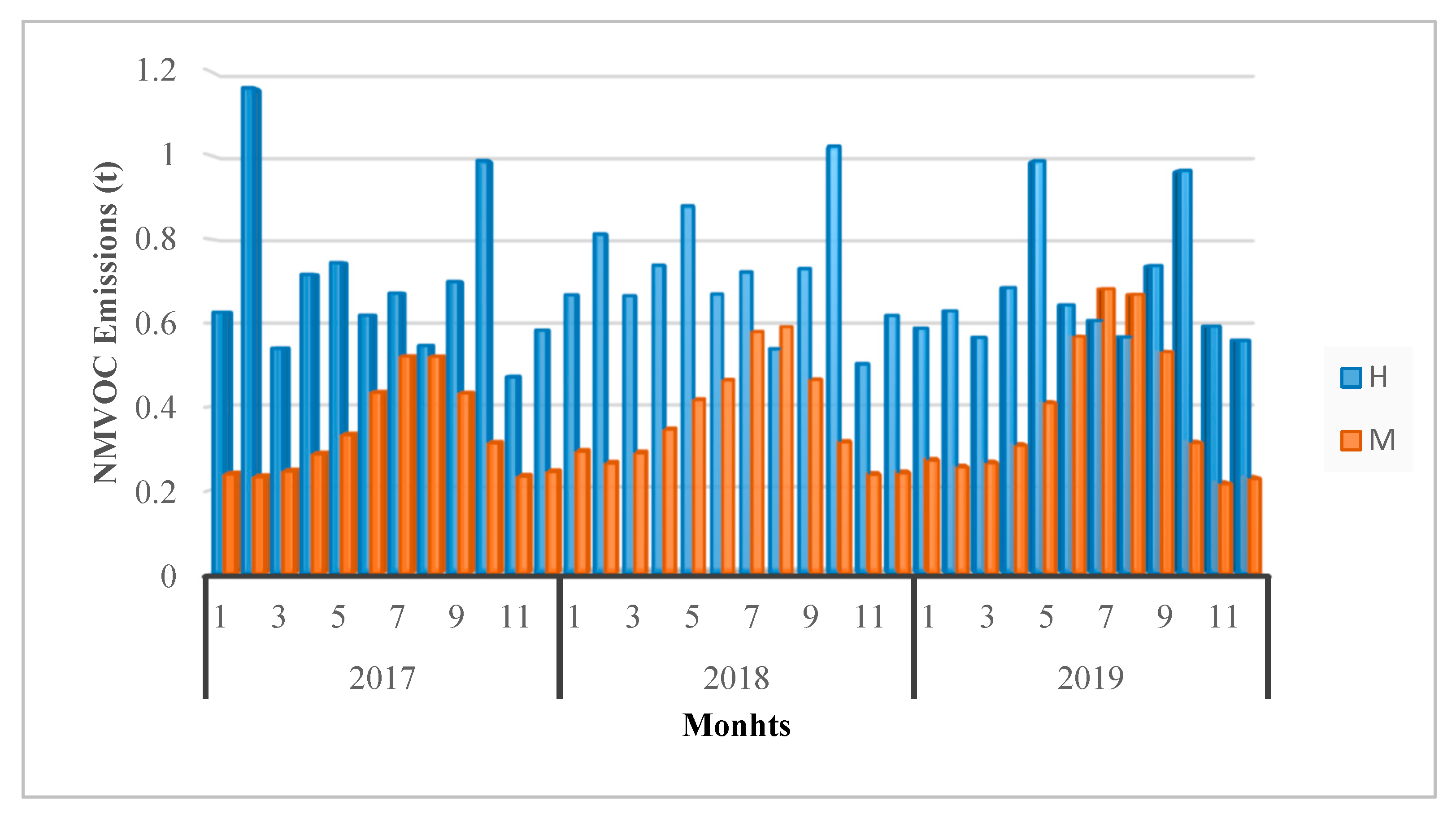
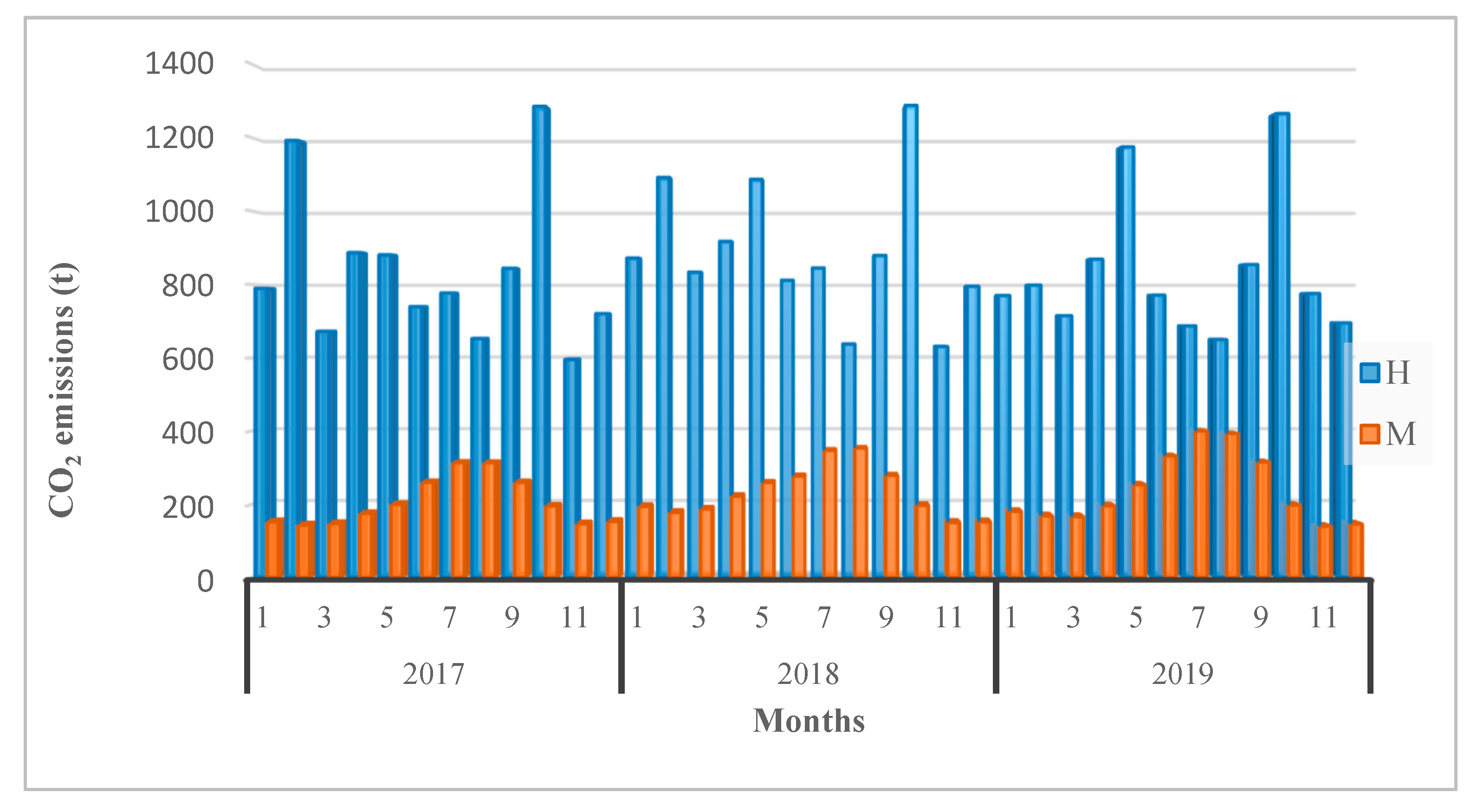
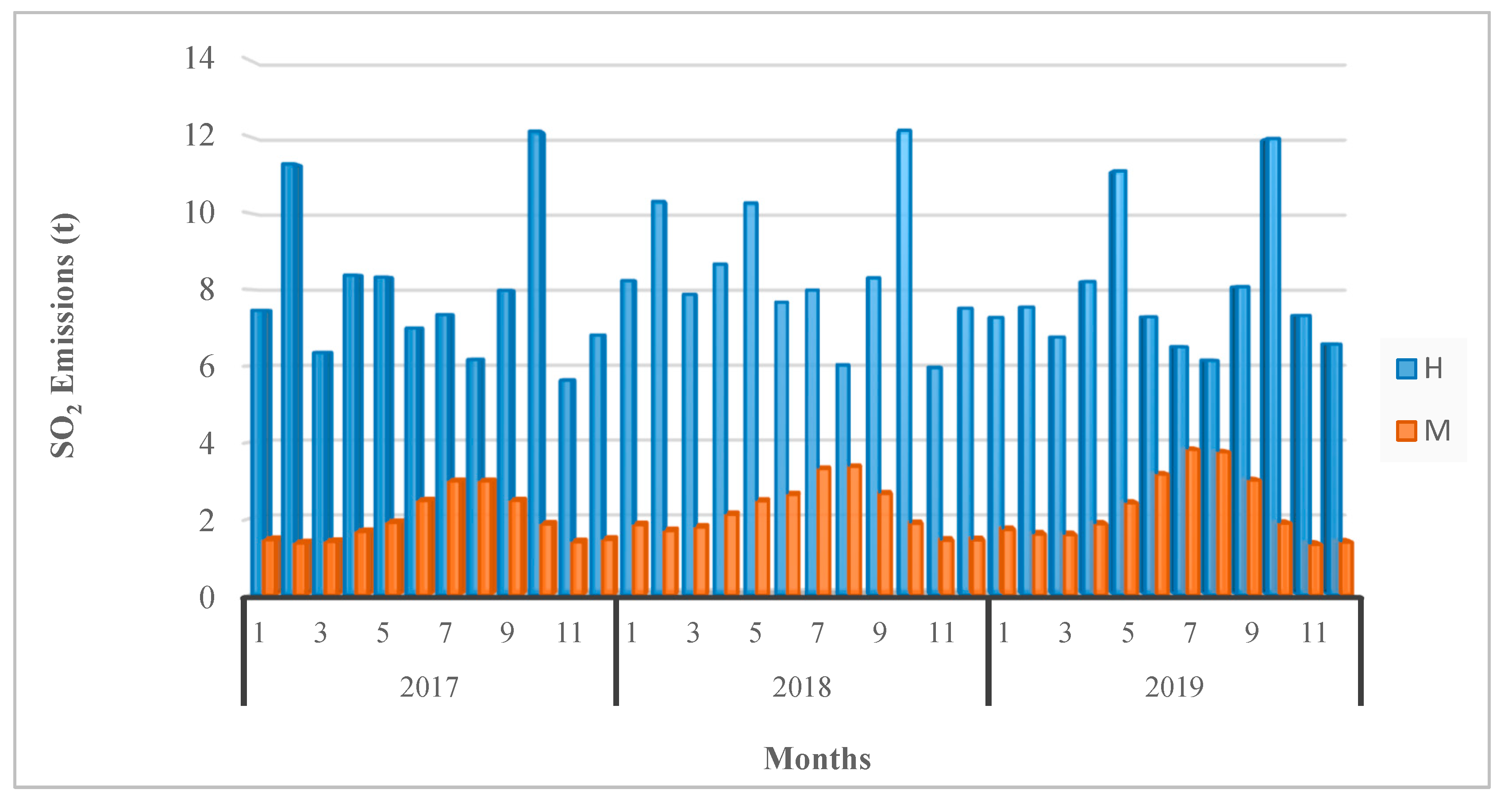
5.1. Results

In this study, the ship emissions are calculated using the activity-based emission estimation for the City port of Split, which is the most significant passenger port in Croatia. The ship emissions are estimated for the ship manoeuvring and hotelling phase. The hotelling phase is responsible for the largest emissions in the port: NOX 90.1%; PM2.5 78.0% and SOX 88.5% [28]. These percentages can vary depending mainly on time spent hotelling and duration of manoeuvring phase [13].
Total emissions in tons of emitted parameters are shown in Table 5. for each month of the observed years. As seen in Table 5. the highest amount of emissions in 2018 was calculated during ship manoeuvring and hotelling operations for all investigated pollutants.
From recent literature, the traffic data for passenger ships other than a cruise, together with annual emissions (tons per year) of NOX and PM10 for the ports Barcelona, Hong Kong, Copenhagen, Venice, Elsinore, St Petersburg, Las Palmas, Genoa, and Marseille are given [13]. These ports have no similarities in size or number of ship arrivals/departures, but the aim was to take into account emissions in urban cities that have ports within the city, such as Split. The minimum NOX emissions are 20 tons per year in the Hong Kong and 1300 tons per year calculated in Marseille port [13]. For PM10 emissions in ports, the range is between 1 ton per year in the Hong Kong port and 80 tons per year in Marseille port [13]. Exhaust gas emissions from ships are calculated for Izmir Port using the ship activity-based methodology. Total emissions from ships in the port is estimated as 1923  tons per year for NOX, 1405  tons per year for SO2, 82,753  tons per year for CO2, 1 ton per year for HC, and 165  tons per year for PM in the year 2007 [30].
The Emissions for each pollutant, divided into manoeuvring and hotelling phase, are shown in Figure 3, Figure 4, Figure 5, Figure 6 and Figure 7. The emissions are divided into years and months and are represented in tons (t). Blue plots represent the hotelling phase (H) and the orange plots represent the manoeuvring phase (M). If side by side comparison is done, the emissions were higher for all pollutants during the hotelling phase than during manoeuvring phase, due to longer time spent in port.
As shown in Figure 8 the hotelling phase contributes to most SO2 emissions with several peaks during the year. On the contrary, the emission trough the manoeuvring phase shows seasonality each year, and it is always relatively smaller than emission during the hotelling phase. The total annual SO2 emission varies from 118 to 127 tons per year, which is way lower than 1405 tons per year in Izmir port [30].
Furthermore, NOX emission varies between 215 tons per year and 235 tons per year (Figure 3), which is almost equal to Barcelona NOX emissions. Ports Hong Kong. Copenhagen, Venice, and Elsinore have lower NOX emissions in ports. Ports St Petersburg, Las Palmas, Genoa and Marseille, have higher NOX emissions. Croatian port of Zadar has total annual cruise ships emissions 310.23 tons per year for NOx, and 9.62 tons per year for PM [35]. Port of Split has lower NOX emissions and higher PM emissions compared to the port of Zadar.
The study of PM10 emission in Ancona’s port reveals that most emissions (70%) happen during the hotelling phase [41]. These emissions correlate with the PM10 emissions from the port of Split (Figure 4). During the hoteling PM emission represents 69% in 2017, 68% in 2018 and 65% in 2019 of total PM emissions in Venice port, Ports Hong Kong, Elsinore, St Petersburg, and Las Palmas have lower PM emissions. Contrary, ports with higher PM10 emissions are Barcelona, Genoa, Copenhagen, and Marseille [13].
From Figure 5, the total annual NMVOC emission varies from 12 to 13 tons per year. In manoeuvring phase emissions are slightly higher during the tourist season period than hotelling phase emissions. This can be explained that in the tourist season period, the number of ship lines has been increased, and therefore, ships spend less time in the ports. As a consequence, the hotelling time is reduced and, therefore, emissions. Additionally, more port arrivals/departures increase manoeuvring time and thus manoeuvring phase emissions.
CO2 emissions contribute majorly to total emissions. From Figure 6, the total annual CO2 emission varies from 12.5 to 13.5 kt. From study [48] and monthly results, there is a difference between the in-season and off-season periods. All emissions slightly increase starting from May and then decrease from October towards the end of the year. The highest manoeuvring emissions are in July and August for all observed years. Such emission trend corresponds to the Croatian shipping company “Jadrolinija” which has the largest number of ship arrivals in the Split city port. The number of ferry lines increases since the end of May, with the peak arrivals in July, August, and September. From the beginning of October, the number of lines decreases.
Unlike manoeuvring emissions, hotelling emissions are not showing seasonality. When hotelling emissions are estimated monthly, there are no significant differences between the in-season and off-season periods. All emissions increase between May and October and emission increase correlates with more time spent in port. The highest hotelling phase emissions in 2017 were in February. It is well known that February is a month when the ship spends almost all the time in the port. Consequently, when hotelling phase emission data are observed, it is evident that the months with a reduction in emissions are the months with a time reduction in port retention.

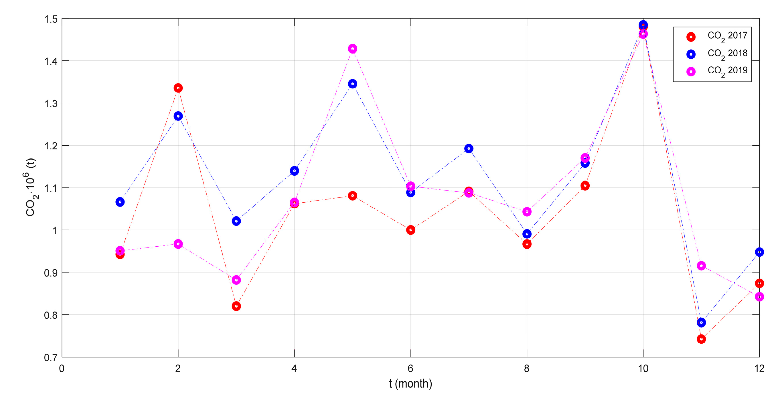
5.2. Analysis of Data

In the next section, a trend and statistical analysis will be performed on CO2 emissions over 2017, 2018, and 2019. Figure 7 shows CO2 emissions through 2017, 2018, and 2019 over the 12 months.
From Figure 7, it can be observed that all CO2 emissions show seasonal character. Additionally, it can be observed that during the in-season period (April, May, June, July, August, and September) the CO2 emission is constant. The average value in 2017 of CO2 emissions is 961.67 t, in 2018 1037.48 t, and in 2019 it is 938.46 t. The total average value during the observed three years is 997.67 t.
To check the relationship between independent (month) variable and dependent variables (CO2 emissions for 2017, 2018, and 2019), an F-test is performed, as shown in Table 6.
From Table 6 it can be seen that all p values are significant, which implies that there are no hidden correlations between independent variable, i.e., month, and all dependent variables, i.e., CO2 emissions for 2017, 2018, and 2019.
Next, trend analysis on the dependent variable, i.e., CO2 emissions, has been performed using regression. The trend analysis is performed to check hypothesis two. Figure 9 shows a graphical presentation of trend analysis of CO2 emissions through observed years, using Equation (9) and regressions.
From Figure 9, it can be observed that blue circles show the values after performing moving average filtering (Equation (9)) of CO2 emissions for observed years. A period of three months is chosen as windows length (WL) for the moving average algorithm. The choice for WL = 3 is derived from the fact that in Republic Croatia, we observe three (3) months, which corresponds with in-season and off-season periods and to eliminate extreme values. Furthermore, the red line shows the trend (regression) of CO2 emissions for the observed years. From the trend of CO2 emissions in 2017, it can be observed that the emissions are constant, although the slope constant has a small negative value (−0.0085). Additionally, the same conclusion could be drawn for 2018. Contrary, for 2019, it can be seen that the slope constant has a small positive value (+0.0068), but since the constant is negligible, it can be concluded that CO2 emission is constant over the year. Overall, the average emission of CO2 stays constant, although the number of vessels during 2019 is increased.
To get further insight into CO2 emission, for observed years, a correlation analysis is performed (Equations (6)–(9)), as shown in Table 7.
From Table 7, it can be observed there are strong correlations between all variables. For example, the correlation coefficient between the CO2 emission from 2017 and CO2 emission from 2018 is 0.906. Additionally, the “weakest” correlation is between the CO2 emission from 2017 and CO2 emission from 2019 (0.670). Further, ANOVA analysis is performed to check the hidden correlations within variables and see. The ANOVA analysis (F = 0.521, Fcrit = 3.285, p = 0.598) shows there are no variations between variables, which implies that all variables come from the same population. That can be explained by the fact that the Split city port operates within full capacity.
It is obvious that some organizational and technological solutions have to be applied to reduce harmful gas emissions, such as better voyage planning (more vessels in less time, especially during the season), usage of more environmentally friendly fuel, etc.
Besides these measures, it is important to find new improvements and solutions such as better cooperation with agents, cargo suppliers. i.e., the creation of integrated management. In terms of technological options, one should be open to renewable sources (fuel cells, wind energy, solar, …) if possible, use environmentally friendly materials of more environmentally efficient technology and find more efficient solutions when building a ship.

6. Conclusions

This paper investigates the ship emissions of pollutants and gases developed by line ships during manoeuvring and hotelling phases in cities that have ports in their centres. The analysis was conducted on the example of the Port of Split.
In the hotelling phase, when the ship is on the berth, the auxiliary engines have higher contribution to emissions than during the “at sea” phase. During manoeuvring phase propulsion engines are operating at low loads and auxiliary engine loads are at their highest load for additional onboard equipment such as thrusters. At berth propulsion engines are usually off and auxiliary engine loads are high during discharging cargo, cars, etc. it is presumed that vessels have their auxiliary engines on during the whole of the time spent in the port.
Through the manoeuvring, it can be observed the emissions show seasonality. That seasonality corresponds to increasing the ferry lines number from the end of May, with the largest arrivals in July, August, and September. Hotelling phase emissions are not shown seasonal patterns, but they depend on ship’s number and port retention.
Comparing all emissions, carbon dioxide (CO2), nitrogen oxides (NOX), volatile organic compounds (VOC), sulphur dioxide (SO2), and particulate matter (PM) it can be seen they are linearly correlated. From the data, it is evident that only CO2 emission had a major impact on pollution.
Trend analysis for CO2 emissions in 2017, 2018, and 2019 shows that the average emissions are constant, despite the number of vessels and staying time in the port.
Correlation analysis shows there are strong correlations between the CO2 emission variables. Additionally, the ANOVA test confirms the findings. That implies all variables come from the same population, which points out that the Split city port operates within full capacity.
The conducted analysis shows that the variables observed during the manoeuvring and hoteling phases in the city port must be taken into account when developing city strategies to make maritime transport (line ships) more efficient, which could contribute in the future to reduce emissions.

Author Contributions

Conceptualization. B.B., M.K. and M.S.; methodology. B.B., M.K. and M.S.; validation. M.K. formal analysis B.B., M.K. and M.S.; investigation. B.B.; writing—original draft preparation. B.B., M.K. and M.S.; visualization. B.B., M.K. and M.S. All authors have read and agreed to the published version of the manuscript.

Funding

This research received no external funding.

Acknowledgments

We wish to extend our special thanks to our reviewers for their comments on an earlier version of the manuscript and improvements they made.

Conflicts of Interest

The authors declare no conflict of interest.

References

  1. Walker, T.R.; Adebambo, O.; Feijoo, M.C.D.A.; Elhaimer, E.; Hossain, T.; Edwards, S.J.; Morrison, C.E.; Romo, J.; Sharma, N.; Taylor, S.; et al. Environmental Effects of Marine Transportation. World Seas Environ. Eval. 2019, 3, 505–530. [Google Scholar] [CrossRef]
  2. Andersson, K.; Baldi, F.; Brynolf, S.; Lindgren, J.F.; Granhag, L.; Svensson, E. Shipping and the Environment. In Shipping and the Environment: Improving Environmental Performance in Marine Transportation; Springer Science and Business Media LLC: Berlin/Heidelberg, Germany, 2016. [Google Scholar] [CrossRef]
  3. Lonati, G.; Cernuschi, S.; Sidi, S. Air quality impact assessment of at-berth ship emissions: Case-study for the project of a new freight port. Sci. Total. Environ. 2010, 409, 192–200. [Google Scholar] [CrossRef] [PubMed]
  4. Sorte, S.; Rodrigues, V.; Borrego, C.; Monteiro, A. Impact of harbour activities on local air quality: A review. Environ. Pollut. 2020, 257, 113542. [Google Scholar] [CrossRef] [PubMed]
  5. Eyring, V.; Isaksen, I.S.A.; Berntsen, T.; Collins, W.J.; Corbett, J.J.; Endresen, Ø.; Grainger, R.G.; Moldanova, J.; Schlager, H.; Stevenson, D.S. Transport impacts on atmosphere and climate: Shipping. Atmos. Environ. 2010, 44, 4735–4771. [Google Scholar] [CrossRef]
  6. WHO. Available online: https://www.who.int/news-room/detail/02-05-2018-9-out-of-10-people-worldwide-breathe-polluted-air-but-more-countries-are-taking-action (accessed on 2 September 2020).
  7. Russo, M.; Leitão, J.; Gama, C.; Ferreira, J.; Monteiro, A. Shipping emissions over Europe: A state-of-the-art and comparative analysis. Atmos. Environ. 2018, 177, 187–194. [Google Scholar] [CrossRef]
  8. Viana, M.; Hammingh, P.; Colette, A.; Querol, X.; Degraeuwe, B.; De Vlieger, I.; Van Aardenne, J. Impact of maritime transport emissions on coastal air quality in Europe. Atmos. Environ. 2014, 90, 96–105. [Google Scholar] [CrossRef]
  9. Merk, O. Shipping Emissions in Ports; International Transport Forum Discussion Papers 2014/20; OECD Publishing: Paris, France, 2014. [Google Scholar] [CrossRef]
  10. 4th IMO Greenhouse Gas Study 2020, Mepc 75/7/15. 2020, Volume 74. Available online: https://safety4sea.com/wp-content/uploads/2020/08/MEPC-75-7-15-Fourth-IMO-GHG-Study-2020-Final-report-Secretariat.pdf (accessed on 30 September 2020).
  11. Eyring, V.; Köhler, H.W.; Van Aardenne, J.; Lauer, A. Emissions from international shipping: 1. The last 50 years. J. Geophys. Res. Space Phys. 2005, 110, 171–182. [Google Scholar] [CrossRef]
  12. Corbett, J.J.; Winebrake, J.J.; Green, E.H.; Kasibhatla, P.; Eyring, V.; Lauer, A. Mortality from Ship Emissions: A Global Assessment. Environ. Sci. Technol. 2007, 41, 8512–8518. [Google Scholar] [CrossRef]
  13. Toscano, D.; Murena, F. Atmospheric ship emissions in ports: A review. Correlation with data of ship traffic. Atmos. Environ. X 2019, 4, 100050. [Google Scholar] [CrossRef]
  14. Anderson, B.; Den Boer, E.; Ng, S.; Dunlap, L.; Hon, G.; Nelissen, D.; Agrawal, A.; Faber, J.; Ray, J. Study of Emission Control and Energy Efficiency Measures for Ships in the Port Area; International Maritime Organization (IMO): London, UK, February 2015. [Google Scholar]
  15. Merico, E.; Gambaro, A.; Argiriou, A.; Alebic-Juretic, A.; Barbaro, E.; Cesari, D.; Chasapidis, L.; Dimopoulos, S.; Dinoi, A.; Donateo, A.; et al. Atmospheric impact of ship traffic in four Adriatic-Ionian port-cities: Comparison and harmonization of different approaches. Transp. Res. Part D Transp. Environ. 2017, 50, 431–445. [Google Scholar] [CrossRef]
  16. Convention, M. International Convention for the Prevention of Pollution from Ships; MARPOL Conv. Outl.; International Maritime Organization (IMO): London, UK, 1973. [Google Scholar]
  17. IMO. The 2020 Global Sulphur Limit: FAQ. 2016, pp. 1–5. Available online: http://www.imo.org/en/MediaCentre/HotTopics/GHG/Documents/FAQ_2020_English.pdf (accessed on 26 September 2020).
  18. Nitrogen Oxides (NOx)—Regulation 13. Available online: http://www.imo.org/en/OurWork/Environment/PollutionPrevention/AirPollution/Pages/Nitrogen-oxides-(NOx)-–-Regulation-13.aspx (accessed on 22 September 2020).
  19. European Environment Agency. Air quality in Europe—2017; Publications Office of the European Union: Luxembourg, 2017. [Google Scholar] [CrossRef]
  20. Miola, A.; Ciuffo, B. Estimating air emissions from ships: Meta-analysis of modelling approaches and available data sources. Atmos. Environ. 2011, 45, 2242–2251. [Google Scholar] [CrossRef]
  21. Tichavska, M.; Tovar, B. External costs from vessel emissions at port: A review of the methodological and empirical state of the art. Transp. Rev. 2017, 37, 383–402. [Google Scholar] [CrossRef] [Green Version]
  22. Tichavska, M.; Tovar, B. Port-city exhaust emission model: An application to cruise and ferry operations in Las Palmas Port. Transp. Res. Part A Policy Pr. 2015, 78, 347–360. [Google Scholar] [CrossRef]
  23. Kiliç, A.; Deniz, C. Inventory of shipping emissions in Izmit Gulf, Turkey. Environ. Prog. Sustain. Energy 2009, 29, 221–232. [Google Scholar] [CrossRef]
  24. Berechman, J.; Tseng, P.-H. Estimating the environmental costs of port related emissions: The case of Kaohsiung. Transp. Res. Part D Transp. Environ. 2012, 17, 35–38. [Google Scholar] [CrossRef]
  25. Song, S. Ship emissions inventory, social cost and eco-efficiency in Shanghai Yangshan port. Atmos. Environ. 2014, 82, 288–297. [Google Scholar] [CrossRef]
  26. Saxe, H.; Larsen, T. Air pollution from ships in three Danish ports. Atmos. Environ. 2004, 38, 4057–4067. [Google Scholar] [CrossRef]
  27. Maragkogianni, A.; Papaefthimiou, S. Evaluating the social cost of cruise ships air emissions in major ports of Greece. Transp. Res. Part D Transp. Environ. 2015, 36, 10–17. [Google Scholar] [CrossRef]
  28. Papaefthimiou, S.; Maragkogianni, A.; Andriosopoulos, K. Evaluation of cruise ships emissions in the Mediterranean basin: The case of Greek ports. Int. J. Sustain. Transp. 2016, 10, 985–994. [Google Scholar] [CrossRef]
  29. Dragović, B.; Tzannatos, E.; Park, N.K. Simulation modelling in ports and container terminals: Literature overview and analysis by research field, application area and tool. Flex. Serv. Manuf. J. 2016, 29, 4–34. [Google Scholar] [CrossRef]
  30. Saraçoğlu, H.; Deniz, C.; Kılıç, A. An Investigation on the Effects of Ship Sourced Emissions in Izmir Port, Turkey. Sci. World J. 2013, 2013, 218324. [Google Scholar] [CrossRef]
  31. Kilic, A.; Tzannatos, E. ShiP emissions and their externalities at the container terminal of Piraeus—Greece. Int. J. Environ. Res. 2014, 8, 1329–1340. [Google Scholar]
  32. Nunes, R.; Alvim-Ferraz, M.; Martins, F.; Sousa, S. Assessment of shipping emissions on four ports of Portugal. Environ. Pollut. 2017, 231, 1370–1379. [Google Scholar] [CrossRef] [PubMed]
  33. Alver, F.; Saraç, B.; Şahin Ülkü, A. Estimating of shipping emissions in the Samsun Port from 2010 to 2015. Atmos. Pollut. Res. 2018, 9, 822–828. [Google Scholar] [CrossRef]
  34. Deniz, C.; Kilic, A. Estimation and assessment of shipping emissions in the region of Ambarlı Port, Turkey. Environ. Prog. Sustain. Energy 2009, 29, 107–115. [Google Scholar] [CrossRef]
  35. Knežević, V.; Radonja, R.; Dundović, Č. Emission Inventory of Marine Traffic for the Port of Zadar. Pomorstvo 2018, 32, 239–244. [Google Scholar] [CrossRef] [Green Version]
  36. Song, S.-K.; Shon, Z.-H. Current and future emission estimates of exhaust gases and particles from shipping at the largest port in Korea. Environ. Sci. Pollut. Res. 2014, 21, 6612–6622. [Google Scholar] [CrossRef]
  37. Villalba, G.; Gemechu, E.D. Estimating GHG emissions of marine ports—The case of Barcelona. Energy Policy 2011, 39, 1363–1368. [Google Scholar] [CrossRef]
  38. Državni Zavod Za Statistiku—Republika Hrvatska. Available online: https://www.dzs.hr/ (accessed on 2 September 2020).
  39. Adriatic Sea Tourism Report; Risposte Turismo. 2017. Available online: http://www.adriaticseaforum.com/2017/Public/RisposteTurismo_AdriaticSeaTourismReport2017.pdf (accessed on 21 September 2020).
  40. Split Tourist Visits in 2019—Split Croatia Travel Guide. Available online: https://split.gg/split-tourist-visits-2019/ (accessed on 2 September 2020).
  41. Carletti, S.; Latini, G.; Passerini, G. Air pollution and port operations: A case study and strategies to clean up. Sustain. City VII 2012, 1, 391–403. [Google Scholar] [CrossRef]
  42. ENTEC. UK Ship Emissions Inventory Final Report. 2010. Available online: https://uk-air.defra.gov.uk/assets/documents/reports/cat15/1012131459_21897_Final_Report_291110.pdf (accessed on 25 September 2020).
  43. HRB Web izvještaj/CRS Web Reports. Available online: http://report.crs.hr/hrbwebreports/ (accessed on 2 September 2020).
  44. ePlovilo. Available online: https://eplovilo.pomorstvo.hr/#/public/dashboard (accessed on 2 September 2020).
  45. Quantification of Emissions from Ships Associated with Ship Movements between Ports in the European Community. Available online: https://ec.europa.eu/environment/air/pdf/chapter1_ship_emissions.pdf (accessed on 21 September 2020).
  46. Pavlić, I. Statistička teorija i primjena; Tehnička knjiga: Zagreb, Croatia, 1988. [Google Scholar]
  47. Strang, G. Linear Algebra and Learning from Data; Wellesley Cambridge Press: Wellesley, MA, USA, 2019. [Google Scholar]
  48. Marušić, E.; Šoda, J.; Krčum, M. The Three-Parameter Classification Model of Seasonal Fluctuations in the Croatian Nautical Port System. Sustainability 2020, 12, 5079. [Google Scholar] [CrossRef]
Figure 1. Environmental impact of shipping.
Jmse 08 00953 g001
Figure 2. Ship arrivals in the City port of Split from 2010 to 2019.
Jmse 08 00953 g002
Figure 3. NOX emissions through years for the hotelling and manoeuvring phase in Split port.
Jmse 08 00953 g003
Figure 4. PM emissions through years the hotelling and the manoeuvring phase in Split port.
Jmse 08 00953 g004
Figure 5. NMVOC emissions through years for hotelling and manoeuvring phase.
Jmse 08 00953 g005
Figure 6. CO2 emissions through years for hotelling and manoeuvring phase.
Jmse 08 00953 g006
Figure 7. CO2 emission in 2017, 2018, 2019 for Split city port.
Jmse 08 00953 g007
Figure 8. SO2 emissions through years for hotelling and manoeuvring phase.
Jmse 08 00953 g008
Figure 9. Trend presentation of CO2 emissions for 2017, 2018, and 2019 of the Split city port.
Jmse 08 00953 g009
Table 1. The list of organizations conventions and laws regarding air pollution from ships.
NameAbbreviationFounded/Entered into ForceRole/Aim
International Maritime OrganizationIMO1948Organization with the role of standardizing procedures and rules for safety at sea
International Convention for the Prevention of Pollution from ShipsMARPOL1973International Convention developed my IMO divided into VI Annexes regarding the different pollutions from the ships
Technical code on control of emissions of Nitrogen OxidesNOX Technical Code2008Document adopted by IMO and in accordance with MARPOL Convention for control of NOX emissions
Sulphur Content of Marine fuels directiveSCMF directive2005EU directive regarding fuel regulation used by passenger vessels on regular services between EU ports. According to the directive while at berths in ports, all ships must use fuel with sulphur content less than 0.1 by weight. The same strict limit of 0.10% m/m. has already been applied in the emission control areas (ECAS), set by the International Maritime Organization.
Environmental Protection Act 2013Croatian act which regulates environmental protection principles
Air Protection Act 2011Croatian act which regulates air protection
Table 2. The main and the auxiliary engine load factors. and the main engine time of operation.
PhaseLFME (%)TOME (%)LFAE (%)
Manoeuvring2010050
Hotelling (except tankers)20540
Table 3. Main and auxiliary engine emission factors for manoeuvring and at berth [45].
Engine TypeFuel TypeNOX Pre 2000 EngineNOX Post 2000 EngineSO2
(g/kWh)
CO2
(g/kWh)
VOC
(g/kWh)
PM
(g/kWh)
Main engine emission factors for manoeuvring and at berth 2007
MSDMDO10.68.86.87101.51.2
Auxiliary engine emission factors for manoeuvring and at berth 2007
M/H SDMDO13.911.56.56900.40.4
Table 4. The example of the excel table for the ship Biokovo—hoteling phases on 19 January 2017.
SHIPBIOKOVO
Main engine (kW)1968
Auxiliary engine (kW)532
Main engine EF NOX (g/kWh)8.8
Main engine EF NMVOC (g/kWh)1.5
Main engine EF TSP PM10 PM2.5 (g/kWh)1.2
Maine engine EF SO26.8
Maine engine EF CO2710
LF main engine (%)0.2
Main engine time of operation (%)0.05
LF auxiliary engine (%)0.4
Auxiliary engine EF NOX (g/kWh)11.5
Auxiliary engine EF NMVOC (g/kWh)0.4
Auxiliary engine EF TSP PM10 PM2.5 (g/kWh)0.4
Auxiliary engine EF SO26.5
Auxiliary engine EF CO2690
NOX (g)23,394.78835
NMVOC (g)1023.50592
PM (g)970.795008
SO2 (g)13,543.9903
CO2 (g)1,435,665.25
Arrival19.01. 11:35
Departure19.01. 20:30
Hours8.927
Table 5. Total emissions in grams of emitted parameters for each month of the observed year for the Port of Split.
Year/MonthsNMVOC (t)PM (t)CO2 (t)NOX (t)SO2 (t)
2017 total12.4010.9812,501.68215.84118.30
10.860.78942.3916.078.91
21.391.221335.6523.1312.65
30.790.70820.1314.077.76
41.000.901062.1918.4710.05
51.080.951081.0218.6010.23
61.050.921000.1916.979.47
71.191.041091.2818.3710.34
81.070.93966.8516.149.16
91.131.001104.9018.9610.46
101.301.181480.5626.9213.99
110.700.63742.3913.097.02
120.830.74874.1215.058.27
2018 total13.0711.6213,487.27234.57127.59
10.960.871066.4918.5210.08
21.080.981269.3222.8111.99
30.950.851021.1617.959.66
41.080.971139.9519.9410.78
51.301.151345.5223.3612.73
61.130.991088.8318.5410.31
71.301.131192.6120.1011.30
81.130.98990.7916.479.39
91.191.051158.3819.8710.97
101.341.211484.7526.6414.04
110.740.66781.4913.757.39
120.860.77947.9816.618.96
2019 total12.8411.3712,920.00224.76122.26
10.860.77951.1616.768.99
20.880.80967.0817.209.14
30.830.74881.9215.778.34
40.990.891065.2818.9110.07
51.401.241428.2924.9313.51
61.211.051103.5018.5810.45
71.291.111087.8817.9410.32
81.241.061043.2817.219.89
91.271.111170.3719.7911.09
101.281.161463.3326.5813.83
110.810.73915.5816.378.65
120.790.70842.3214.707.97
Grand Total for 3 years38.3133.9738,908.95675.17368.15
Table 6. F-test Two-Sample for Variances whether the selection of variables is acceptable, i.e., whether there are hidden correlations between them, and whether t is an independent variable.
2017 Year2018 Year2019 Year
MonthCO2 EmissionMonthCO2 EmissionMonthCO2 Emission
Mean6.51.0456.51.1246.51.077
Variance130.008130.008130.013
Observations121212121212
df11 11 1111
F1527.375 1501.531 935.875
p (F ≤ f) one-tail7.367 × 10−16 8.091 × 10⁻¹⁶ 1.085 × 10⁻¹⁴
F Critical one-tail2.817 2.817 2.817
Table 7. Correlation matrix of CO2 emissions for 2017, 2018, and 2019 of the Split city port.
201720182019
20171
20180.9061
20190.6700.8131
Publisher’s Note: MDPI stays neutral with regard to jurisdictional claims in published maps and institutional affiliations.

