Simulating the Trajectory and Biomass Growth of Free-Floating Macroalgal Cultivation Platforms along the U.S. West Coast


 ,
,  and
and 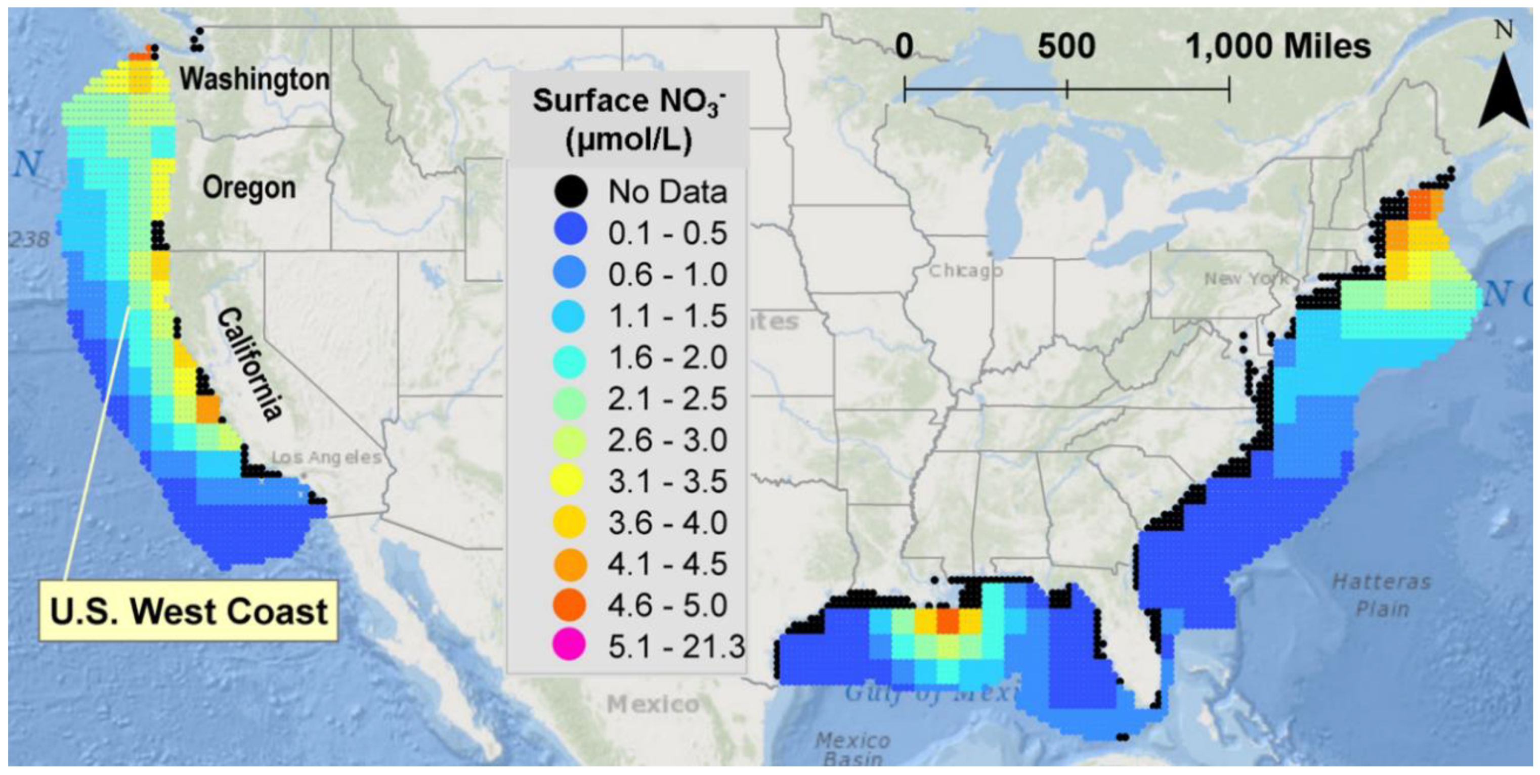
Abstract
:1. Introduction
2. Methods
2.1. NOMAD Project
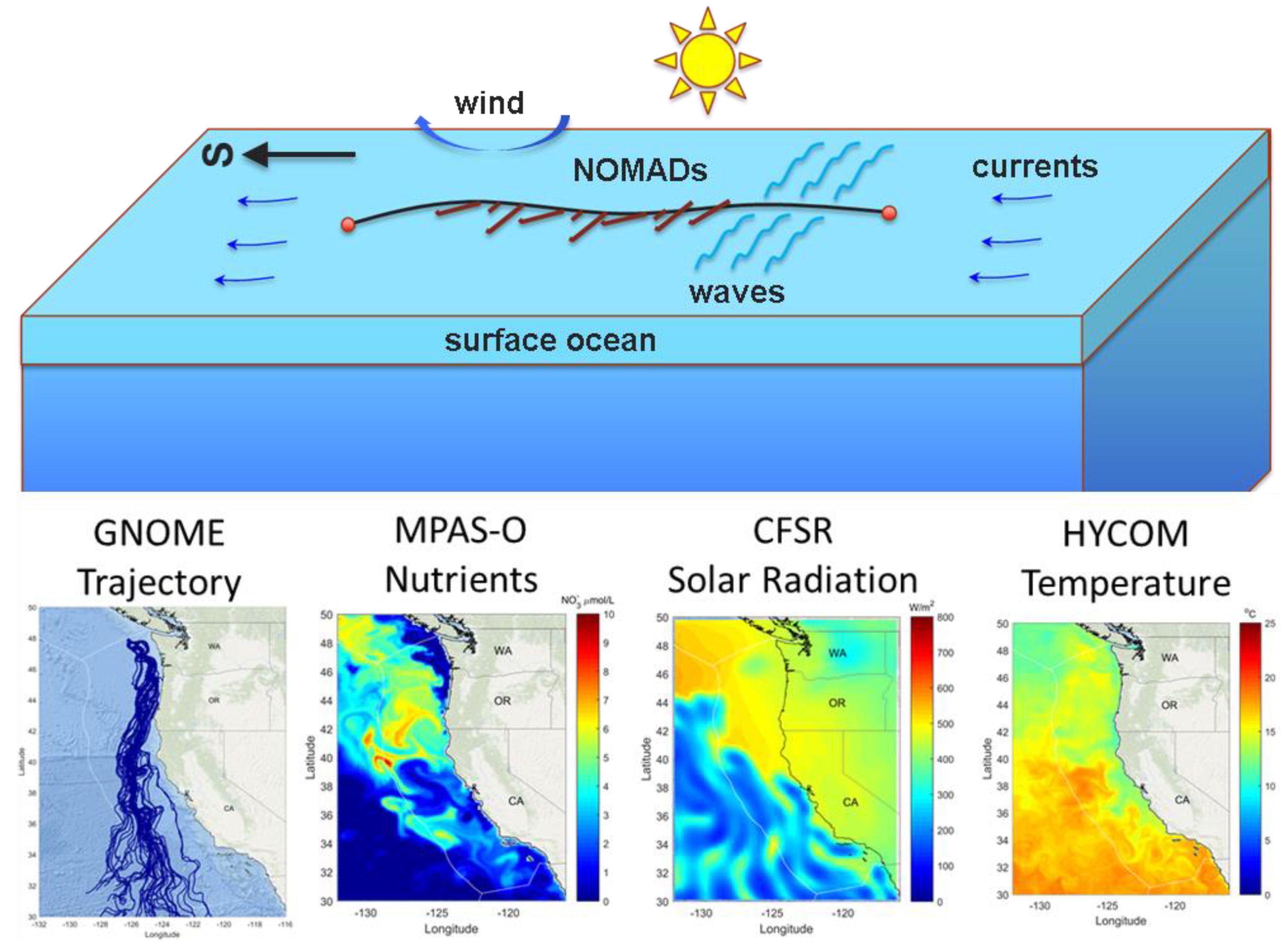
2.2. Trajectory Model
2.3. Macroalgal Growth Model
2.4. Simulation Design
3. Results and Discussion
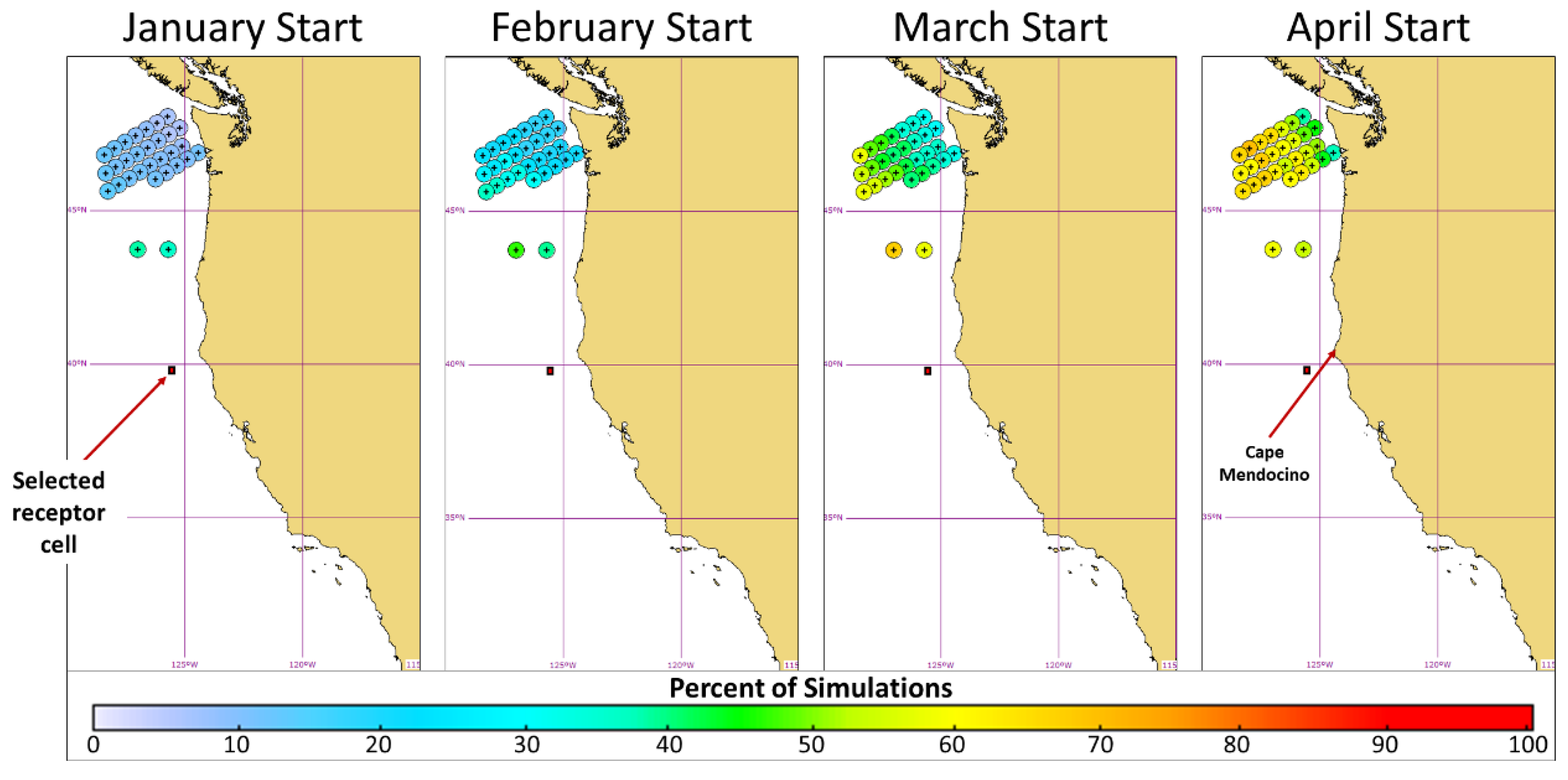
3.1. Release Location Analysis
3.2. Pathway Analysis
3.3. Timing Analysis
3.4. Growth Analysis
4. Conclusions
Author Contributions
Funding
Acknowledgments
Conflicts of Interest
References
- Oilage Guide to Fuels from Macroalgae; Report by Oilage: Chennai, India, 2010.
- Sherman, M.T.; Blaylock, R.; Lucas, K.; Capron, M.E.; Stewart, J.R.; DiMarco, S.F.; Thyng, K.; Hetland, R.; Kim, M.H.; Sullivan, C.; et al. SeaweedPaddock: Initial Modeling and Design for a Sargassum Ranch. In Proceedings of the OCEANS 2018 MTS/IEEE Charleston, Charleston, SC, USA, 22–25 October 2018; pp. 1–6. [Google Scholar] [CrossRef]
- van Sebille, E.; Aliani, S.; Law, K.L.; Maximenko, N.; Alsina, J.; Bagaev, A.; Bergmann, M.; Chapron, B.; Chubarenko, I.; Cózar, A.; et al. The physical oceanography of the transport offloating marine debris. Environ. Res. Lett. 2020, 15, 023003. [Google Scholar] [CrossRef] [Green Version]
- Galt, J.A.; Watabayashi, G.Y.; Payton, D.L.; Petersen, J.C. Trajectory Analysis for the Exxon Valdez: Hindcast Study. Int. Oil Spill Conf. Proc. March 1991, 1991, 629–634. [Google Scholar] [CrossRef]
- Liu, Y.; Weisberg, R.; Hu, C.; Zheng, L. Tracking the Deepwater Horizon Oil Spill: A Modeling Perspective. EOS 2011, 92, 45–56. [Google Scholar] [CrossRef]
- Lumpkin, R. Global characteristics of coherent vortices from surface drifter trajectories. J. Geophys. Res. Oceans 2016, 121, 1306–1321. [Google Scholar] [CrossRef] [Green Version]
- Mulet, S.; Rio, M.; Mignot, A.; Guinehut, S.; Morrow, R. A new estimate of the global 3D geostrophic ocean circulation based on satellite data and in-situ measurements. Deep Sea Res. Part II Top. Stud. Oceanogr. 2012, 77, 70–81. [Google Scholar] [CrossRef]
- van Sebille, E.; Griffies, S.M.; Abernathey, R.; Adams, T.; Berloff, P.; Biastoch, A.; Blanke, B.; Chassignet, E.; Cheng, Y.; Cotter, C.; et al. Lagrangian ocean analysis: Fundamentals and practices. Ocean Model. 2018, 121, 49–75. [Google Scholar] [CrossRef]
- Ebbesmeyer, C.; Ingraham, J., Jr. Pacific toy spill fuels ocean current pathways research. EOS 1994, 75, 425–430. [Google Scholar] [CrossRef]
- Beegle-Krause, J. General NOAA Oil Modeling Environment (GNOME): A New Spill Trajectory Model. Int. Oil Spill Conf. Proc. March 2001, 2001, 865–871. [Google Scholar] [CrossRef]
- Maximenko, N.; Hafner, J. SCUD: Surface Currents from Diagnostic Model; Technical Note No. 5; International Pacific Research Center (IPRC): Honolulu, HI, USA, 2010; p. 19. [Google Scholar]
- Usui, N.; Ishizaki, S.; Fujii, Y.; Tsujino, H.; Yasuda, T.; Kamachi, M. Meteorological Research Institute multivariate ocean variational estimation (MOVE) system: Some early results. Adv. Space Res. 2006, 37, 806–822. [Google Scholar] [CrossRef]
- Sim, L.; Graham, J.; Rose, K.; Duran, R.; Nelson, J.; Umhoefer, J.; Vielma, J. Developing a Comprehensive Deepwater Blowout and Spill Model; Technical Report for NETL-TRS-9-2015 EPAct Technical Report Series; U.S. Department of Energy, National Energy Technology Laboratory: Albany, OR, USA, 2015.
- Maximenko, N.; Hafner, J.; Kamachi, M.; MacFadyen, A. Numerical simulations of debris drift from the Great Japan Tsunami of 2011 and their verification with observational report. Mar. Pollut. Bull. 2018, 132, 5–25. [Google Scholar] [CrossRef]
- Duran, R.; Romeo, L.; Whiting, J.; Vielma, J.; Rose, K.; Bunn, A.; Bauer, J. Simulation of the 2003 Foss Barge—Point Wells Oil Spill: A Comparison between BLOSOM and GNOME Oil Spill Models. J. Mar. Sci. Eng. 2018, 6, 104. [Google Scholar] [CrossRef] [Green Version]
- Jackson, G.A. Modeling the Growth and Harvest Yield of the Giant-Kelp Macrocystis Pyrifera. Mar. Biol. 1987, 95, 611–624. [Google Scholar] [CrossRef]
- Solidoro, C.; Pecenik, G.; Pastres, R.; Franco, D.; Dejak, C. Modelling macroalgae (Ulva rigida) in the Venice lagoon: Model structure identification and first parameters estimation. Ecol. Model. 1997, 94, 191–206. [Google Scholar] [CrossRef]
- Trancoso, A.R.; Saraiva, S.; Fernandes, L.; Pina, P.; Leitão, P.; Neves, R. Modelling macroalgae using 3D hydrodynamic-ecological model in a shallow, temperate estuary. Ecol. Model. 2005, 187, 232–246. [Google Scholar] [CrossRef]
- Wang, T. Numerical Modeling of Eutrophication Dynamics in the Shallow Coastal Ecosystem: A Case Study in the Maryland and Virginia Coastal Bays. Ph.D. Thesis, The College of William & Mary, Gloucester Point, VA, USA, 2009. [Google Scholar] [CrossRef]
- Broch, O.J.; Slagstad, D. Modelling seasonal growth and composition of the kelp Saccharina latissima. J. Appl. Phycol. 2012, 24, 759–776. [Google Scholar] [CrossRef]
- Broch, O.J.; Ellingsen, I.H.; Forbord, S.; Wang, X.; Volent, Z.; Alver, M.O.; Handa, A.; Andresen, K.; Slagstad, D.; Reitan, K.I.; et al. Modelling the cultivation and bioremediation potential of the kelp Saccharina latissima in close proximity to an exposed salmon farm in Norway. Aquac. Environ. Interact. 2013, 4, 187–206. [Google Scholar] [CrossRef] [Green Version]
- Hadley, S.; Wild-Allen, K.; Johnson, C.; Macleod, C. Modeling macroalgae growth and nutrient dynamics for integrated multi-trophic aquaculture. J. Appl. Phycol. 2014, 27, 901–916. [Google Scholar] [CrossRef]
- Brooks, M.T.; Coles, V.J.; Hood, R.R.; Gower, J.F.R. Factors controlling the seasonal distribution of pelagic Sargassum. Mar. Ecol. Prog. Ser. 2018, 599, 1–18. [Google Scholar] [CrossRef] [Green Version]
- Macroalgae Research Inspiring Novel Energy Resources (MARINER). Available online: https://arpa-e.energy.gov/?q=arpa-e-programs/mariner (accessed on 9 September 2020).
- Roesijadi, G.; Copping, A.E.; Huesemann, M.H.; Forster, J.; Benemann, J.R. Technoeconomic Feasibility Analysis of Offshore Seaweed Farming for Bioenergy and Biobased Products; Independent Research and Development Report PNWD-3931; Battelle Pacific Northwest Division: St Richland, WA, USA, 2008; p. 115. [Google Scholar]
- Chen, M.; Yim, S.C.; Cox, D.; Huesemann, M.; Yang, Z.; Wang, T.; Mumford, T.; Wood, G. Hydrodynamic Load Modeling for Offshore Free-Floating Macroalgal Aquaculture under Extreme Environmental Conditions. In Proceedings of the Offshore Mechanics and Arctic Engineering Conference, Glasgow, Scotland, 9–14 June 2019. [Google Scholar] [CrossRef]
- Greene, J.M.; Gulden, J.; Wood, G.; Huesemann, M.; Quinn, J.C. Techno-Economic and Life Cycle Assessment of a Novel Offshore Macroalgae Biorefinery. Algal Res. 2020, 51, 102032. [Google Scholar] [CrossRef]
- Hickey, B.M.; Banas, N.S. Oceanography of the U.S. Pacific Northwest Coastal Ocean and estuaries with application to coastal ecology. Estuaries 2003, 26, 1010–1031. [Google Scholar] [CrossRef]
- Sayre, R.G.; Wright, D.J.; Breyer, S.P.; Butler, K.A.; Van Graafeiland, K.; Costello, M.J.; Harris, P.T.; Goodin, K.L.; Guinotte, J.M.; Basher, Z.; et al. A three-dimensional mapping of the ocean based on environmental data. Oceanography 2017, 30, 90–103. [Google Scholar] [CrossRef]
- Garcia, H.E.; Locarnini, R.A.; Boyer, T.P.; Antonov, J.I.; Baranova, O.K.; Zweng, M.M.; Reagan, J.R.; Johnson, D.R. World Ocean Atlas 2013, Volume 4: Dissolved Inorganic Nutrients (phosphate, nitrate, silicate). In NOAA Atlas NESDIS 76; Levitus, S., Mishonov, A., Eds.; U.S. Government Publishing Office: Washington, DC, USA, 2014; p. 25. [Google Scholar]
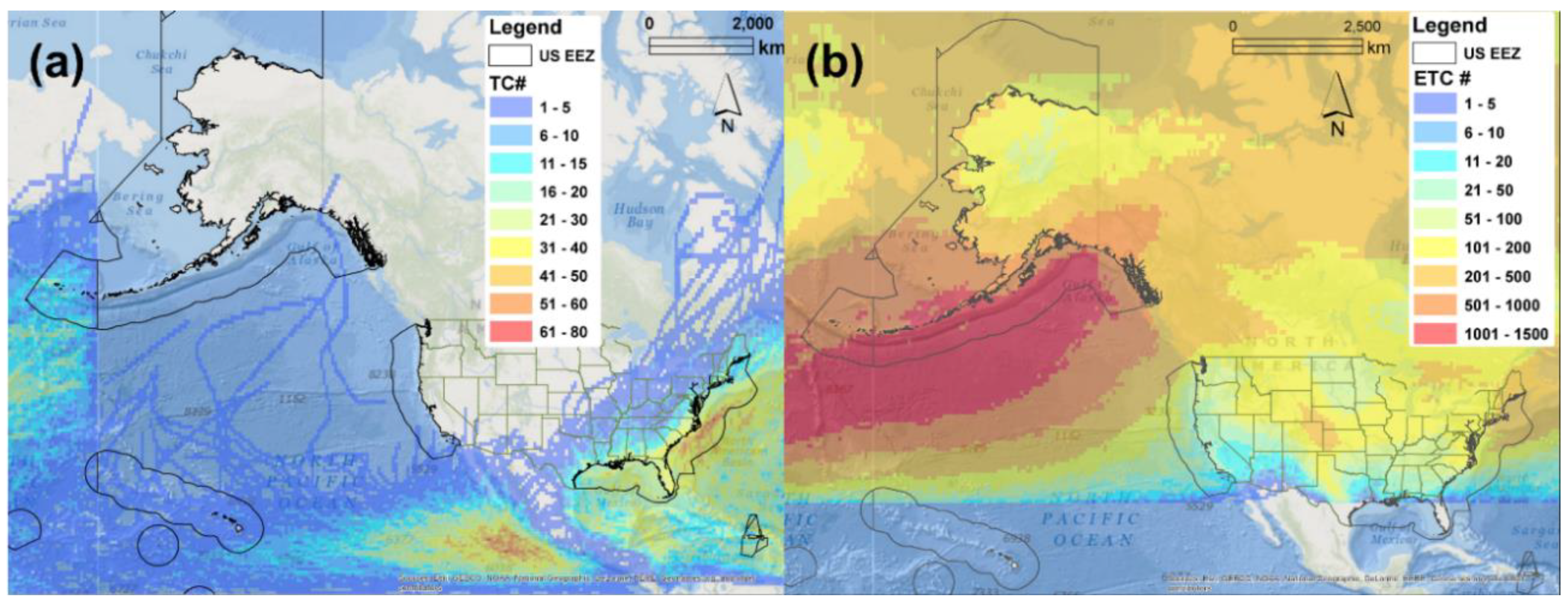
- Knapp, K.R.; Kruk, M.C.; Levinson, D.H.; Diamond, H.J.; Neumann, C.J. The International Best Track Archive for Climate Stewardship (IBTrACS): Unifying tropical cyclone data. Bull. Am. Meteorol. Soc. 2010, 91, 363–376. [Google Scholar] [CrossRef]
- Compo, G.P.; Whitaker, J.S.; Sardeshmukh, P.D.; Matsui, N.; Allan, R.J.; Yin, X.; Gleason, B.E.; Vose, R.S.; Rutledge, G.; Bessemoulin, P.; et al. The Twentieth Century Reanalysis Project. R. Meteorol. Soc. 2011, 137, 1–28. [Google Scholar] [CrossRef]
- Beegle-Krause, C.J. GNOME: NOAA’s Next-Generation Spill Trajectory Model. In MTS/IEEE Conference Committee, Proceedings of Oceans ‘99 MTS/IEEE, Escondido, CA, USA, 13–16 September 1999; IEEE: New York, NY, USA, 1999; Volume 3, pp. 1262–1266. [Google Scholar] [CrossRef]
- NOAA Marine Debris Program. Severe Marine Debris Event Report: Japan Tsunami Marine Debris; Overview and Update to Congress; NOAA Marine Debris Program: Silver Spring, MD, USA, 2013; p. 46.
- Cummings, J.A.; Smedstad, O.M. Variational Data Assimilation for the Global Ocean. In Data Assimilation for Atmospheric, Oceanic and Hydrologic Applications; Park, S., Xu, L., Eds.; Springer: Berlin/Heidelberg, Germany, 2013; Volume 2, pp. 303–343. [Google Scholar] [CrossRef]
- Saha, S.; Moorthi, S.; Pan, H.; Wu, X.; Wang, J.; Nadiga, S.; Tripp, P.; Kistler, R.; Woollen, J.; Behringer, D.; et al. NCEP Climate Forecast System Reanalysis (CFSR) Selected Hourly Time-Series Products, January 1979 to December 2010; Research Data Archive at the National Center for Atmospheric Research, Computational and Information Systems Laboratory, 2010. Available online: https://rda.ucar.edu/ (accessed on 7 November 2020). [CrossRef]
- Bowie, G.L.; Mills, W.B.; Porcella, D.B.; Campbell, C.L.; Pagenkopt, J.R.; Rupp, G.L.; Johnson, K.M.; Chan, P.W.H.; Gherini, S.A. Rates, Constants and Kinetics Formulations in Surface Water Quality Modeling, 2nd ed.; EPA 600/3-85/040; US Environmental Protection Agency: Athens, GA, USA, 1985.
- Cerco, C.F.; Noel, M.R. The 2002 Chesapeake Bay Eutrophication Model. Report No. EPA 903-R-04-004; Springer: New York, NY, USA, 2004. [Google Scholar]
- Neushul, M.; Benson, J.; Harger, B.W.W.; Charters, A.C. Macroalgae Farming in Sea: Water Motion and Nutrient Uptake. J. Appl. Phycol. 1992, 4, 255–265. [Google Scholar] [CrossRef]
- Ringler, T.; Petersen, M.; Higdon, R.L.; Jacobsen, D.; Jones, P.W.; Maltrud, M. A multi-resolution approach to global ocean modeling. Ocean Model. 2013, 69, 211–232. [Google Scholar] [CrossRef]
- Wang, S.; Bailey, D.; Lindsay, K.; Moore, J.K.; Holland, M. Impact of sea ice on the marine iron cycle and phytoplankton productivity. Biogeosciences 2014, 11, 4713–4731. [Google Scholar] [CrossRef] [Green Version]
- Petersen, M.R.; Asay-Davis, X.S.; Berres, A.S.; Chen, Q.; Feige, N.; Hoffman, M.J.; Jacobsen, D.W.; Jones, P.W.; Maltrud, M.E.; Price, S.F.; et al. An evaluation of the ocean and sea ice climate of E3SM using MPAS and interannual CORE-II forcing. J. Adv. Model Earth Syst. 2019, 11, 1438–1458. [Google Scholar] [CrossRef]
- Gevaert, F.; Creach, A.; Davoult, D.; Holl, A.-C.; Seuront, L.; Lemoine, Y. Photo-inhibition and seasonal photosynthetic performance of the seaweed Laminaria saccharina during a simulated tidal cycle: Chlorophyll fluorescence measurements and pigment analysis. Plant, Cell Environ. 2002, 25, 859–872. [Google Scholar] [CrossRef] [Green Version]
- Brush, M.J.; Nixon, S.W. Biomass layering and metabolism in mats of the macroalga Ulva lactuca L. Estuaries 2003, 26, 916–926. [Google Scholar] [CrossRef]
- Roleda, M.Y.; Hurd, C.L. Seaweed nutrient physiology: Application of concepts to aquaculture and bioremediation. Phycologia 2019, 58, 552–562. [Google Scholar] [CrossRef] [Green Version]
- Ahn, O.; Petrell, R.J.; Harrison, P.J. Ammonium and nitrate uptake by Laminaria saccharina and Nereocystis luetkeana originating from a salmon sea cage farm. J. Appl. Phycol. 1998, 10, 333–340. [Google Scholar] [CrossRef]
- Rosenberg, G.; Probyn, T.A.; Mann, K.H. Nutrient uptake and growth kinetics in brown seaweeds: Response to continuous and single additions of ammonium. J. Exp. Mar. Biol. Ecol. 1984, 80, 125–146. [Google Scholar] [CrossRef]
- Droop, M.R. An approach to quantitative nutrition of phytoplankton. J. Protozool. 1977, 24, 528–532. [Google Scholar] [CrossRef]
- Trajectory Analysis Planner (TAP). Available online: https://response.restoration.noaa.gov/oil-and-chemical-spills/oil-spills/response-tools/trajectory-analysis-planner.html (accessed on 9 September 2020).
- Rothäusler, E.; Gutow, L.; Thiel, M. Floating Seaweeds and Their Communities. In Seaweed Biology: Ecological Studies (Analysis and Synthesis) Vol 219; Wiencke, C., Bischof, K., Eds.; Springer: Berlin/Heidelberg, Germany, 2012. [Google Scholar] [CrossRef]
- Visch, W.; Nylund, G.M.; Pavia, H. Growth and biofouling in kelp aquaculture (Saccharina latissima): The effect of location and wave exposure. J. Appl. Phycol. 2020, 32, 3199–3209. [Google Scholar] [CrossRef]
- Edwards, M.S. Comparing the impacts of four ENSO events on giant kelp (Macrocystis pyrifera) in the northeast Pacific Ocean. Algae 2019, 34, 141–151. [Google Scholar] [CrossRef]
- Kim, J.K.; Kraemer, G.P.; Yarish, C. Use of sugar kelp aquaculture in Long Island Sound and the Bronx River Estuary for nutrient extraction. Mar. Ecol. Prog. Ser. 2015, 531, 155–166. [Google Scholar] [CrossRef]
- Peteiro, C.; Freire, Ó. Biomass yield and morphological features of the seaweed Saccharina latissima cultivated at two different sites in a coastal bay in the Atlantic coast of Spain. J. Appl. Phycol. 2013, 25, 205–213. [Google Scholar] [CrossRef]
- Broch, O.J.; Alver, M.O.; Bekkby, T.; Gundersen, H.; Forbord, S.; Handå, A.; Skjermo, J.; Hancke, K. The kelp cultivation potential in coastal and offshore regions of Norway. Front. Mar. Sci. 2019, 5, 529. [Google Scholar] [CrossRef]
- Röhrs, J.; Christensen, K.; Hole, L.; Broström, G.; Drivdal, M.; Sundby, S. Observation-based evaluation of surface wave effects on currents and trajectory forecasts. Ocean Dyn. 2012, 62, 1519–1533. [Google Scholar] [CrossRef]


Publisher’s Note: MDPI stays neutral with regard to jurisdictional claims in published maps and institutional affiliations. |
© 2020 by the authors. Licensee MDPI, Basel, Switzerland. This article is an open access article distributed under the terms and conditions of the Creative Commons Attribution (CC BY) license (http://creativecommons.org/licenses/by/4.0/).
Share and Cite
Whiting, J.M.; Wang, T.; Yang, Z.; Huesemann, M.H.; Wolfram, P.J.; Mumford, T.F.; Righi, D. Simulating the Trajectory and Biomass Growth of Free-Floating Macroalgal Cultivation Platforms along the U.S. West Coast. J. Mar. Sci. Eng. 2020, 8, 938. https://doi.org/10.3390/jmse8110938
Whiting JM, Wang T, Yang Z, Huesemann MH, Wolfram PJ, Mumford TF, Righi D. Simulating the Trajectory and Biomass Growth of Free-Floating Macroalgal Cultivation Platforms along the U.S. West Coast. Journal of Marine Science and Engineering. 2020; 8(11):938. https://doi.org/10.3390/jmse8110938
Chicago/Turabian StyleWhiting, Jonathan M., Taiping Wang, Zhaoqing Yang, Michael H. Huesemann, Phillip J. Wolfram, Thomas F. Mumford, and Dylan Righi. 2020. "Simulating the Trajectory and Biomass Growth of Free-Floating Macroalgal Cultivation Platforms along the U.S. West Coast" Journal of Marine Science and Engineering 8, no. 11: 938. https://doi.org/10.3390/jmse8110938