Combining Numerical Simulations and Normalized Scalar Product Strategy: A New Tool for Predicting Beach Inundation

Abstract

The skills of the Normalized Scalar Product (NSP) strategy, commonly used to estimate the wave field, as well as bathymetry and sea-surface current, from X-band radar images, are investigated with the aim to better understand coastal inundation during extreme events. Numerical simulations performed using a Nonlinear Shallow-Water Equations (NSWE) solver are run over a real-world barred beach (baseline tests). Both bathymetry and wave fields, induced by reproducing specific storm conditions, are estimated in the offshore portion of the domain exploiting the capabilities of the NSP approach. Such estimates are then used as input conditions for additional NSWE simulations aimed at propagating waves up to the coast (flood simulations). Two different wave spectra, which mimic the actual storm conditions occurring along the coast of Senigallia (Adriatic Sea, central Italy), have been simulated. The beach inundations obtained from baseline and flood tests related to both storm conditions are compared. The results confirm that good predictions can be obtained using the combined NSP–NSWE approach. Such findings demonstrate that for practical purposes, the combined use of an X-band radar and NSWE simulations provides suitable beach-inundation predictions and may represent a useful tool for public authorities dealing with the coastal environment, e.g., for hazard mapping or warning purposes.

1. Introduction

The nearshore area hosts many human activities and interests, which have become increasingly important in recent years. Climate change can have a potentially destabilizing effect on such activities: both sea level rise and increase of sea storminess may promote an increase of the coastal inundation frequency, this severely affecting engineering works, as well as ecological, recreational and environmental issues [1,2]. Hence, analyses of coastal vulnerability and inundation risk are required worldwide to prevent and/or mitigate such changes, and represent a fundamental task to be accounted for when coastal plans and policies are carried out [3,4,5,6,7].

Specifically, coastal flooding and erosion can potentially induce important economic losses and human fatalities. An Integrated Coastal Zone Management (ICZM) approach, which spans over the main aspects of the coastal region (from prediction to protection, from engineering to ecosystems, from tourism to sustainability) seems essential to mitigate the mentioned negative impacts. The need for an integrated approach in the coastal area is globally acknowledged, also in view of the increasing pressures which are featuring our world, e.g., population growth, concentration of economic activities, expanding tourism [8]. As an example, an important protocol has been signed in the framework of the Barcelona Convention, which promotes an integrated approach of the coastal zone management in the Mediterranean area [9]. Such protocol focuses on the spatial development of coastal zones, and the need for assessing and measuring pressures from human activities. Studies have been undertaken based on the proposed approach and applications have been attempted, e.g., [10,11].

In this framework, estimating the beach inundation of a specific location is fundamental for, e.g., hazard mapping purposes, coastal risk analysis, application of the ICZM approach. Suitable tools are thus required for the monitoring of the nearshore region, with many devices being tested for this purpose in the recent years. For instance, Lagrangian drifters and floaters have long been used for oceanic studies and can properly measure hydrodynamics (waves, currents) and seabed morphology along the coast, e.g., [12,13]. Furthermore, fixed instruments (Eulerian approach) deployed in the sea for a certain time are often used for the reconstruction of the wave field in the nearshore region, with the possibility to record data during both calm and stormy periods, though the risk concerning the equipment safety, e.g., [14,15]. However, devices based on a remote sensing approach, such as acoustic sensors [16], X-band radar [17], video-monitoring systems [18,19], look easier to be used during severe conditions. Diaz et al. [20] assessed a reliable measure when two or more of such devices are contemporary used and their results are combined. Suitable post-processing tools are also required to retrieve useful information in the analyzed domain, e.g., wave characteristics (height, period, direction), breaker features (roller length, energy dissipation), seabed morphology.

Among the remote sensing systems mentioned above, we have here considered the X-band marine radar, which provides an alternative to the standard detection systems of the sea state (e.g., buoys and others). Currently, the X-band marine radar, besides being used for the detection and tracking of the targets on sea surface, is employed as a remote sensing tool for sea-state monitoring both on ships [21,22,23] and in coastal areas [24,25,26,27]. The radar echoes arising from the sea surface and received by antenna radar, if properly processed, allow one to retrieve the sea-state parameters such as length, period and direction of the dominant waves, and the significant wave heights, as well as to reconstruct the sea-surface current and bathymetry field.

With a specific focus on the bathymetry reconstruction, various radar imaging techniques are available, and these significantly evolved in time. In the last three decades, several approaches for current and bathymetry estimation have been developed as Least-Square (LS) [28], Iterative Least-Square (ILS) [29], Normalized Scalar Product (NSP) [30,31]. Since many of the above tools, such as X-band radars, are not able at measuring or reconstructing the hydro-morphodynamics in the shallowest region of the beach, numerical modeling can be used as an additional tool to be exploited for coastal inundation purposes. Specifically, the results/estimates obtained using the remote sensor can be used as input conditions for the numerical model, i.e., a “chain approach”, which is similar to that applied in recent studies. These demonstrate the feasibility to reconstruct the shallow-water hydrodynamics induced by forcing actions of various nature exploiting a series of numerical/analytical models and/or sea observations [7,32,33].

Typical numerical approaches for the description of the coastal regions are based on the solution of either the Nonlinear Shallow-Water Equations (NSWE) [34,35] or the Boussinesq equations [36,37]. On one hand, both model/equation types are based on the assumption of wave nonlinearity, a fundamental feature which describes the wave evolution in intermediate to shallow waters. On the other hand, the wave frequency dispersion, which mainly describes the wave energy re-distribution during the wave propagation, also plays an important role in the description of the wave transformation in the nearshore region, but is only accounted for by Boussinesq-type models. However, shallow-water computations provide suitable results even when a NSWE solver is used, often exploiting a reduced computational cost. Recently, with the aim to exploit the best skills from both approaches, based on the use of both Boussinesq (in intermediate to deep waters) and NSWE (in the shallowest waters) approaches, hybrid models have been built [38,39].

The present paper investigates the potentialities of the combination of the NSP approach and shallow-water simulations in properly predicting the beach inundation. In detail, the NSP estimates are used as boundary conditions (wave-field reconstruction) and initial conditions (bathymetry reconstruction) of a Nonlinear Shallow-Water Equations (NSWE) solver, able at transferring shoreward the reconstructed wave and providing the beach inundation and runup. Different wave conditions and various beach scenarios have been tested, with the purpose to illustrate and validate a novel method to evaluate the coastal inundation exploiting radar images.

The paper is divided as follows. Section 2 describes the used tools, i.e., the hydrodynamic NSWE solver and the NSP approach, as well as their combination. The results obtained using the above tools are reported and discussed in Section 3. A final discussion closes the paper (Section 4).

2. Materials and Methods

The present work is aimed at illustrating a methodology that can be applied for the prediction of the beach inundation. Specifically, remote sensing devices, aimed at reconstructing the bathymetric evolution of a coastal region [20,28,29,30,31], may also be exploited to reconstruct the wave field in the investigated domain, so as to generate suitable initial and boundary conditions to be used by phase-resolving models which propagate the wave up to the swash zone. With such purpose, a NSWE solver is first used to generate the wave field over a real-world bathymetry to simulate what actually occurs in the open sea. The generated wave field is then modulated to simulate the signal recorded by an X-band marine radar. An NSP algorithm is used to reconstruct both wave field and bathymetry. Such reconstructions are then used to run numerical simulations of beach inundation.

2.1. The hydrodynamic Solver

The numerical model used for the wave-field generation within the domain (baseline simulations), as well as for the wave propagation from the boundary condition to the shore (flood simulations), is that described in [34], which is based on the solution of the NSWE, i.e., depth-averaged equations of the mass and momentum conservation. The non-conservative form of the NSWE, which is based on the Cartesian coordinate system $(x,y,z)$, follows:

$$\begin{array}{ccc}\hfill d_{,t}+{\left(ud\right)}_{,x}+{\left(vd\right)}_{,y}& =& 0,\hfill \end{array}$$

(1)

$$\begin{array}{ccc}\hfill u_{,t}+u{u}_{,x}+v{u}_{,y}+g{d}_{,x}& =& g{h}_{,x}-B_x,\hfill \end{array}$$

(2)

$$\begin{array}{ccc}\hfill v_{,t}+u{v}_{,x}+v{v}_{,y}+g{d}_{,y}& =& g{h}_{,y}-B_y,\hfill \end{array}$$

(3)

with $\mathbf{v}=(u,v)$ the depth-averaged horizontal velocity, g the gravity acceleration, d the total water depth, h the still water depth, both providing the surface water level $\eta =d-h$. The friction contributions are provided through a Chezy-type approach, i.e., $B_x=C_f\left|\mathbf{v}\right|u/d$ and $B_y=C_f\left|\mathbf{v}\right|v/d$, where the dimensionless coefficient $C_f$ is described using a constant value (as in many previous works [7,34,35]).

Due to the depth-averaged nature of the NSWE model, the inversion technique exploits the shallow-water approximation of the dispersion relation, i.e.,

$$\omega =k\sqrt{gh}+\overline{k}\times \overline{U},$$

(4)

where $\omega$ is the angular frequency, $\overline{k}=(k_x,k_y)$ the wave vector, $k=|\overline{k}|$ the wave number and $\overline{U}=(U,V)$ the external current. However, since (4) leads to nonunique solutions when the inversion technique is applied to estimate both depth and current, the present simulations do not account for external currents ($|\overline{U}|=0 \mathrm{m}/\mathrm{s}$) and the depth is the only unknown. Hence, the only currents in the numerical domain are those inherently generated by the wave field (for more details, see [31]).

2.2. The NSP Method

The step between baseline and flood simulations is undertaken using the NSP approach, which has already been tested and validated using both real-world and numerical data [25,31,40], and is typically used to elaborate radar images. These are not direct representation of the wave elevation profile, but they are tied to the slopes of the long sea waves (tilt modulation), to the roughness of the riding short waves (hydrodynamic modulation). Moreover, the radar signals are affected by the “shadowing”, for which no information can be recovered for the sea spots that are not in the line of sight (LOS) [17,41,42,43]. These phenomena are called modulation effects and are introduced during the microwave remote sensing process. Herein, only the shadowing and tilt modulation effects are considered. In particular, the shadowing effect can be interpreted as a geometrical phenomenon and is modeled as if the radar antenna was not actually receiving any signal from the shadowed parts of the sea surface. Instead, the tilt modulation depends on the local power received by the radar antenna on the slope of the observed surface. This causes a modulation of the received radar signal, which is dependent on the angle between the radar illumination ray (i.e., the local LOS) and the normal vector to the wave surface. More details on the geometry and formulation of the tilt model and the shadowing can be found in [17,31]. As in [31], the numerical analysis assumes an incoherent marine radar placed at a height of 20 m above the mean sea level and at coordinates $(x,y)=(0,0)$ m.

The strategy employed to retrieve both sea-state parameters and bathymetry in coastal areas from the simulated X-band radar images, involves a spatial partitioning of the radar images into partially overlapping sub-areas [21,24,44,45]. Therefore, each radar image belonging to the temporal sequence under analysis is partitioned into $N_s$ spatially overlapping sub-areas, giving rise to $N_s$ temporal subsequences. Once the data partitioning step is performed, $N_s$ radar spectra ${\left\{F^j(\overline{k},\omega )\right\}}_{j=1,\dots ,N_s}$ corresponding to the sub-areas, are computed via the Fast Fourier Transform (FFT) algorithm. Then, starting from the local radar spectra [17,31], the local bathymetric value ${\widehat{h}}^j$ is founded on the maximization of the following Normalized Scalar Product, i.e.,

$${\widehat{h}}^j=\arg \underset{h}{\max }\frac{\langle \left|F^j(\overline{k},\omega )\right|,G(\overline{k},\omega ,h)\rangle }{\sqrt{P_{F^j}}}$$

(5)

where $G(\overline{k},\omega ,h)=\delta (\omega -k\sqrt{gh})$ is the characteristic function (being $\delta (·)$ the Dirac-delta distribution) based on the dispersion relation, $\langle \left|F^j\right|,G\rangle$ represents the scalar product of the functions $|F^j|$ and G, while $P_{F^j}$ is the power associated with $|F^j|$. It is worth noticing that the NSP strategy allows us the joint estimation of the surface currents and the bathymetry from the radar spectrum [25,46], with the wave fields generated using a null sea-surface current for the present context.

Therefore, the bathymetry field can thus be reconstructed starting from the local estimates. Such information is of course extremely useful for various coastal applications, but it is also an essential tool to correctly estimate the wave field since, as is well known, the depth, as well as the sea-surface current, are required to define a Band-Pass (BP) filter to separate the energy of the sea signal from the noise background in the radar spectrum. The required sea-wave spectrum $F_w^j(\overline{k},\omega )$ can be obtained from the filtered image spectrum $F_I^j(\overline{k},\omega )$ by resorting to the radar Modulation Transfer Function (MTF), which mitigates the distortions affecting the radar echoes and caused by the acquisition geometry (e.g., shadowing and tilt modulation) [17,24,25,47]. For this purpose, the MTF described in [17] and reported in the following equation has been adopted.

$$F_w^j(\overline{k},\omega )=\frac{F_I^j(\overline{k},\omega )}{k^{\beta }}\mathrm{for}\beta =1.2$$

(6)

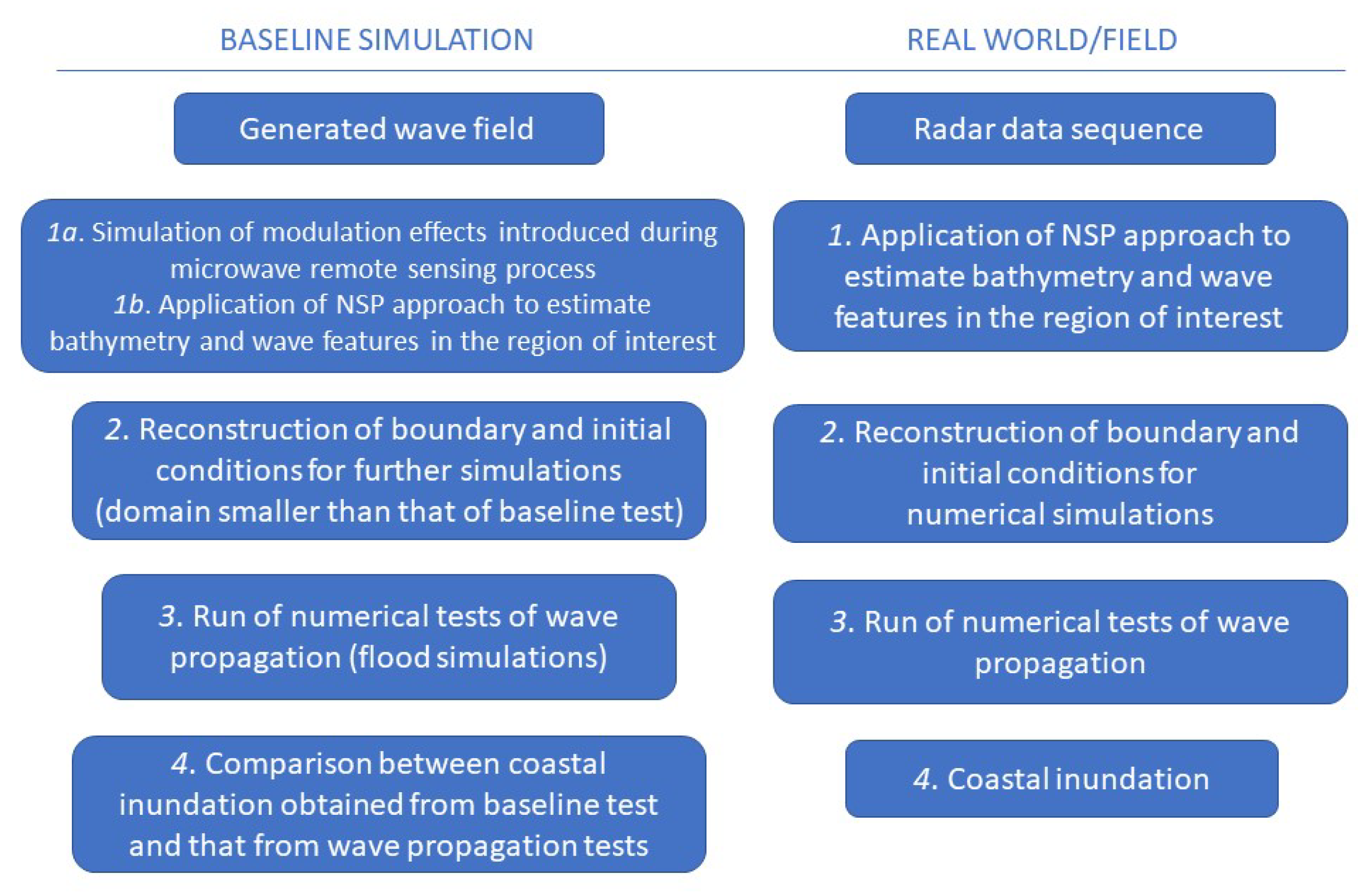
2.3. The Methodology

The methodology which is here proposed aims at combining the application of remote sensors, such as X-band marine radar, for the reconstruction of both offshore wave field and bathymetry, with the numerical modeling in shallow waters. The main goal is that of providing a useful tool for coastal authorities to either reconstruct the nearshore hydrodynamics or predict the coastal inundation. In this case, the above tool needs to be properly integrated and act in real time such as warning systems. The methodology described in the following can be used to reach this purpose.

• The zero-th step is the wave field to be investigated in a specific region of interest: while this exists in the real world, it is here simulated to provide realistic conditions (baseline simulations), similarly to [31].
• The first step is the reconstruction of both wave field and bathymetry in an offshore portion of the domain (order of kilometers from the coast, where typically radar sequence data are collected) using the NSP approach.
• The estimated bathymetry and wave characteristics (significant wave height $H_{m0}$, peak period $T_p$, direction ${\theta }_0$) are used to build, respectively, the seabed morphology and the boundary conditions (in terms of JONSWAP spectra) at different depths/locations.
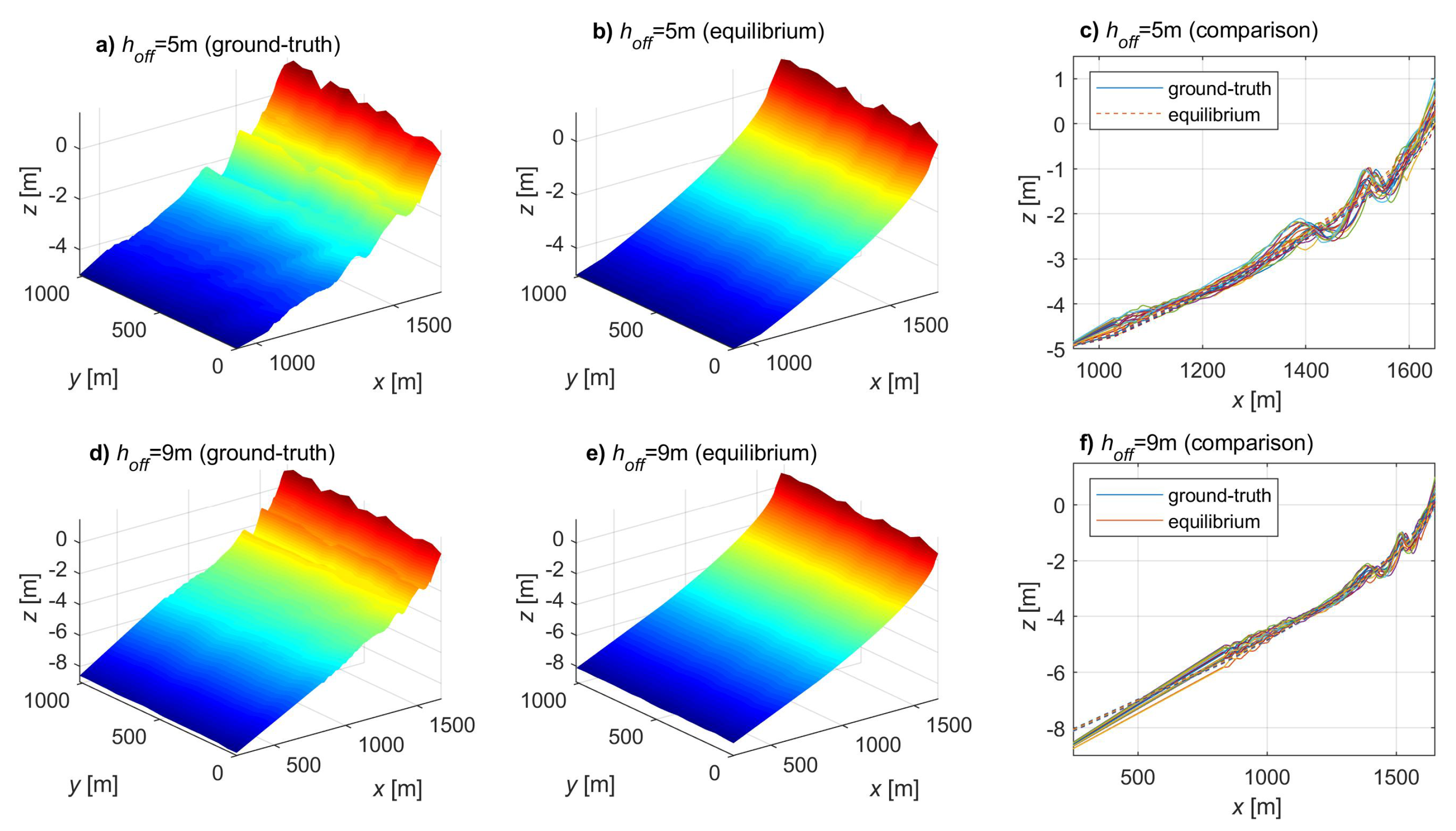
• Flood simulations are run using boundary conditions at depths of either $h=5$ m or $h=9$ m, and using either ground-truth bathymetries or equilibrium-profile bathymetries. While the use of a ground-truth bathymetry represents the case of beach surveys available for the region of interest, the equilibrium profiles may be applied when surveys are not available, as such an approach has already been observed to provide an accurate description of coastal dynamics [48,49].
• The beach inundation obtained from each baseline simulation is compared to the results of the corresponding flood simulations.

Figure 1 summarizes the main steps of the methodology: what is illustrated in the present work (left) and what is expected to do in the real world (right).

2.4. The Application

The described methodology has been applied to one of the most representative coastal areas of the central Italy. Specifically, the coast of Senigallia, one of the most important touristic towns of the Italian Middle Adriatic coast, has been recently studied under several points of view. In particular, the site is characterized by the combination of several forcing actions and processes, especially due to the Misa River (length of ∼48 km, watershed of ∼383 km${}^2$), whose estuarine area is highly engineered and separates the Northern coast of Senigallia, protected by an array of emerged breakwaters, from the Southern part, a natural open coast [15,50]. Such natural, unprotected beach is part of the longest unprotected beach of the Marche Region, extending for about 12 km, from the Misa River estuary to some kilometers North of the Esino River estuary.

The nearshore region used in the present work is located in the Southern beach, where a couple of video-monitoring systems have been recently installed, with the aim to reconstruct the beach dynamics in a large portion of the Southern beach [51]. The swash-zone slope ranges between 1:30 and 1:40. Moving seaward, a multiple array of submerged bars exists in a water depth $h=(0$–$3)$ m, while a mild slope (∼1:200) characterizes larger depths. Fine to medium sands, i.e., $d_{50}=(0.125$–$0.5)$ mm, is typical of the emerged beach, while fine sand, i.e., $d_{50}=(0.125$–$0.25)$ mm, characterizes the submerged beach [50].

Recent studies undertaken on the Southern coast underline that the most frequent and energetic waves are those coming either from ESE or NNE. The former waves are forced by Levante-Scirocco winds, the latter by Bora winds, and both types correspond to the predominant waves of the investigated coastal region. It has also been observed that different wave climates provide different morphological behavior of the submerged beach, mainly concerning the bar migration and evolution. Specifically, the NNE waves experience a reduced refraction and are characterized by a small storm-surge, as a consequence of the reduced fetch due to the elongated shape of the Adriatic basin. Conversely, the refraction process of ESE waves is important, and the longer fetch produces a larger surge. Such considerations translate into a significantly different hydrodynamics, e.g., NNE waves are steeper than ESE waves, and morphodynamics, e.g., larger bar smoothing during NNE waves [50].

The Numerical Simulations

The bathymetry of Senigallia surveyed in May 2013 has been used for the baseline simulations, i.e., the beach developing from the Misa River estuary for about 1 km to the South (see Figure 2). Since such survey was undertaken up to a depth of about 6 m, it was extended seaward, assuming a constant slope of 1:200 up to a 10 m depth.

The baseline tests have been run using two different types of waves which characterize the energetic features of the considered site, as described in [50]. Specifically, for the application of the described methodology, one simulation reproduces a milder wave coming from ESE, the other a steeper wave coming from NNE. The main wave characteristics (significant height $H_{m0}$, peak period $T_p$, wave direction ${\theta }_0$) used for the generation of the boundary conditions at the offshore side of the numerical domain are shown in

Table 1. Wave characteristics used at the offshore boundary of the numerical domain for the baseline simulations.

Wave Type	${\mathit{H}}_{\mathit{m}0,0}$	${\mathit{T}}_{\mathit{p}}$	${\mathit{\theta }}_0$	${\mathit{\theta }}_{0,\mathit{l}}$
	[m]	[s]	[${}^{\circ }$]	[${}^{\circ }$]
ESE	1.51	7.25	67	−22
NNE	2.25	6.75	40	5

. It is worth noting that the direction is also affected by the refraction process, which enables the wave rays to rotate while approaching the coast. A local angle is also introduced, i.e., the angle at which the waves enter the domain. This is estimated as ${\theta }_{0,l}={\theta }_0-{\theta }_{coast}$, where ${\theta }_{coast}\approx {45}^{\circ }$ is the angle between the normal to the coast and the North. As with the numerical simulations presented in [31] and in agreement with recent field observations of swell waves along the Senigallia coast during calm states and storm tales [52], long-crested waves with no directional spreading and $T_p=(5$–$10)$ s have been reproduced.

Since the NSWE solver needs to be fed with both instantaneous water level and depth-averaged velocity, the spectral data of both baseline tests (Table 1) have been transformed into random free-surface time series using the method described in [53], which consists of the following steps: (i) spectrum discretization into a finite number of frequency intervals; (ii) setting of the wave characteristics of each frequency interval; (iii) summation of all waves (e.g., see [7]). An application of such method is illustrated in Figure 3, where the JONSWAP spectrum (Figure 3a) is that related to the wave characteristics of the NNE forcing (Table 1). The time series of the water-surface level has been generated starting from such spectrum using [53]’s method (Figure 3b).

Both numerical simulations have been run using a spatial discretization along the cross-shore and alongshore directions of, respectively, $(\mathsf{\Delta }x,\mathsf{\Delta }y)=(2,5)$ m, and a friction coefficient $C_f=0.005$, consistent with classical coastal processes, e.g., [35].

3. Results

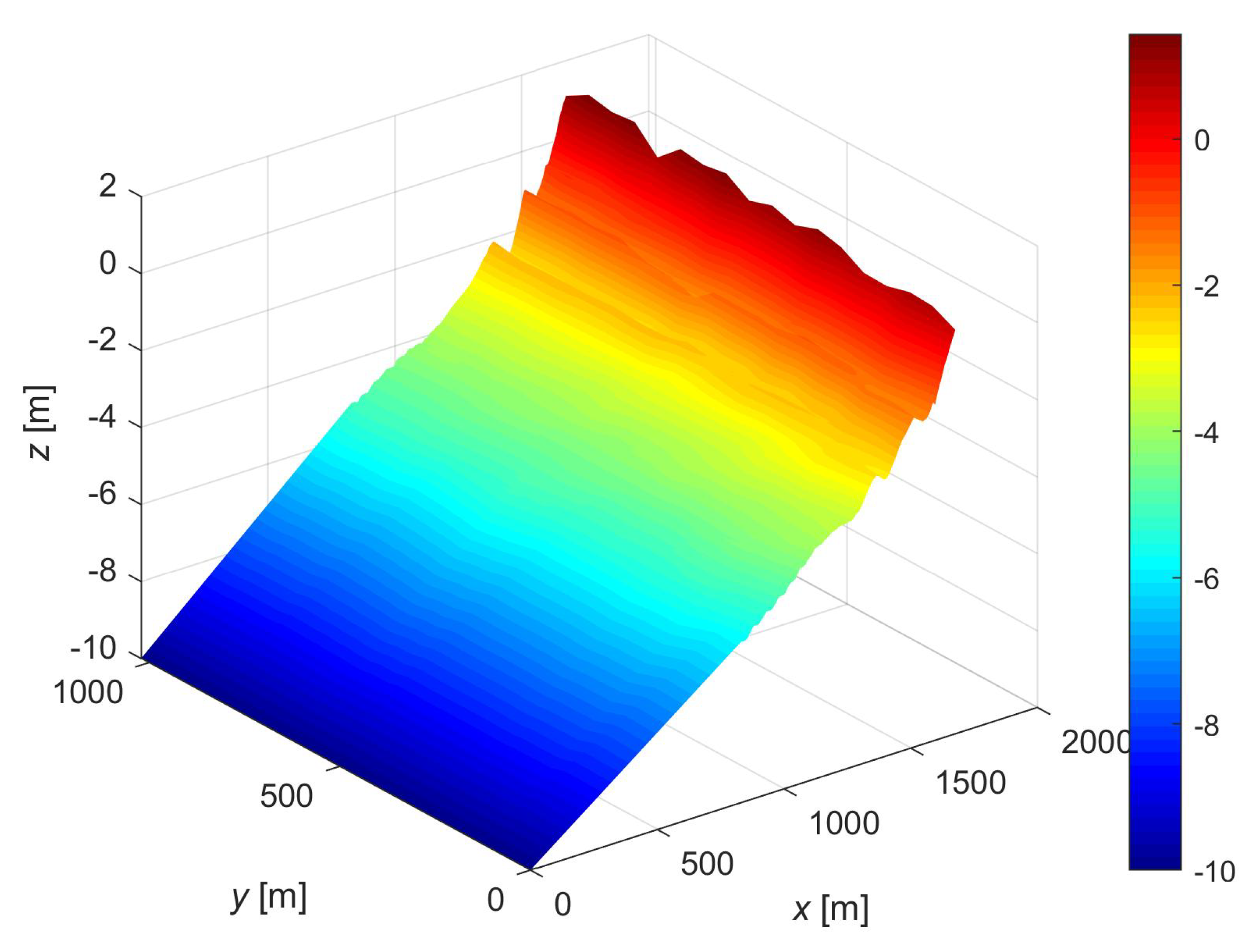
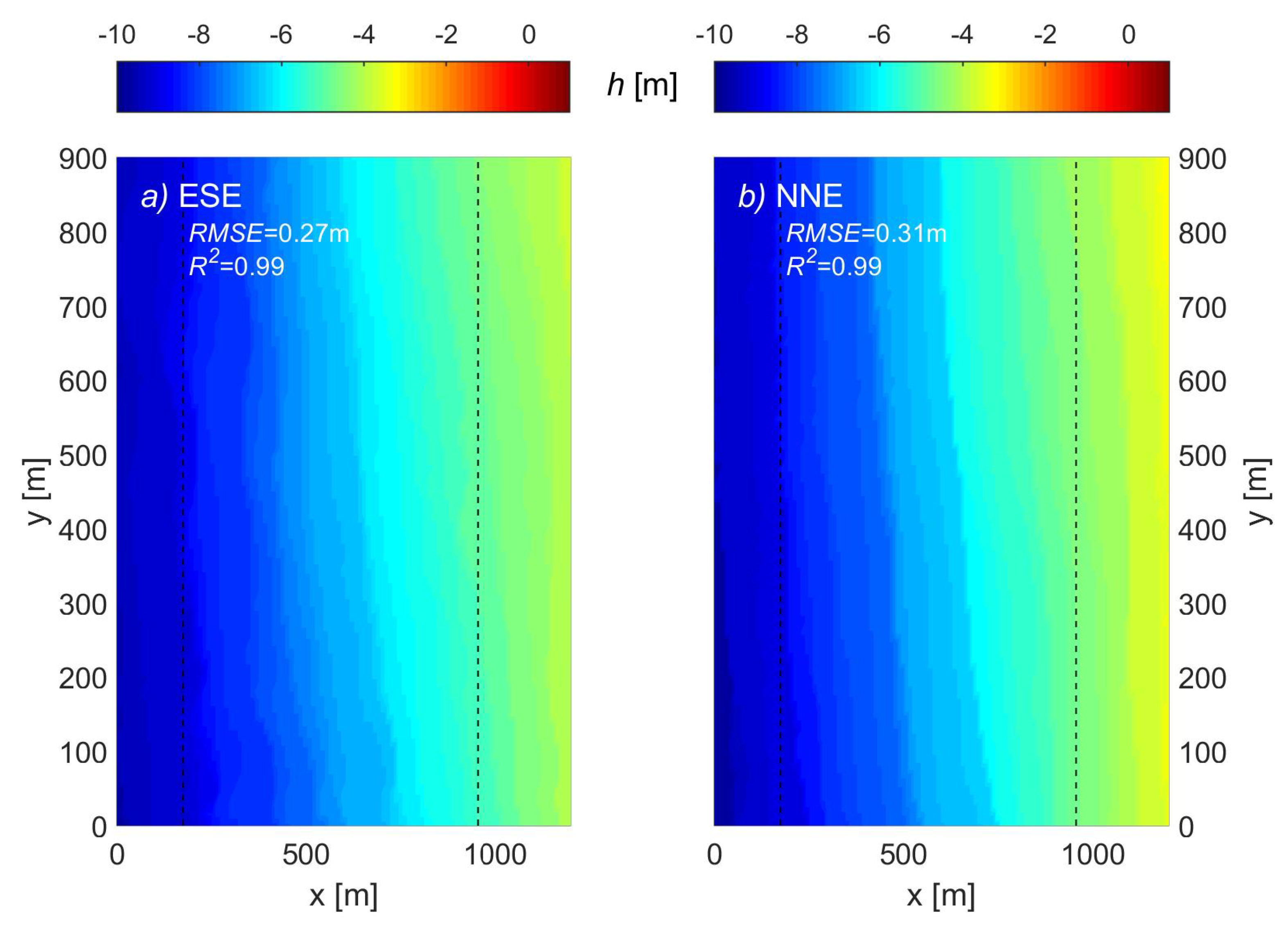
3.1. Step 1: NSP Reconstruction

This section is devoted to present the results obtained from the elaboration of the radar data sequence by means of the NSP strategy described in Section 2. Each considered sequence consists of 256 individual radar images with an interval $\mathsf{\Delta }t=1$ s between two consecutive images and the extent of the pixel in the Cartesian grid is equal to 5 m. An example of both synthetic sea-wave image obtained by means of the NSWE solver (Figure 4a) and amplitude of the corresponding radar image (Figure 4b) is illustrated at the same time instant ($t=128$ s).

To estimate the local sea-state parameters and bathymetry, the spatial partitioning strategy described in Section 2 is applied to the radar data sequence. In particular, a sub-area size equal to $(250\times 250)$ m${}^2$ and $(300\times 300)$ m${}^2$ is adopted for radar sequences belonging to the wave coming from NNE and ESE, respectively. Such difference in the sub-area size is due to the wavelength associated with the directional spectrum evaluated within the whole area investigated by the radar (more details are reported in [31]).

First, the NSP procedure provided the bathymetry reconstructions, which are shown using a pixel spacing of 10 m for both wave types (Figure 5). The reliability of the bathymetric reconstruction using the NSP strategy has been widely demonstrated (e.g., [31]), so the error statistics is reported in Figure 5, for both wave types, only in terms of Root Mean Square Error (RMSE) and correlation coefficient square ($R^2$), obtained from the comparison with the ground-truth (Figure 2).

As said, the purpose of this work is to provide suitable beach-inundation predictions starting from the local estimation of the sea-state parameters from the data acquired by means of an X-band wave-radar system. Hence, in the inversion procedure, after application of the BP filter, the following step consists of the application of the MTF to turn from the filtered radar spectrum to the desired sea-wave spectrum $F_w^j(\overline{k},\omega )$ at each sub-area j. From such spectrum $F_w^j(\overline{k},\omega )$, it is possible to determine the main sea-state parameters at each sub-area, i.e., the peak period $T_p^j$, the peak direction ${\theta }_p^j$, as well as the significant wave height $H_{m0}^j$. These are used for the generation of the boundary conditions to be applied at specific locations along the cross-shore direction. In particular, these parameters are tied to the spectral moment of zero order $m_0$ for $H_{m0}^j$, to the wave number spectrum $F_w^j\left(\overline{k}\right)$ for ${\theta }_p^j$ and to the one-dimensional frequency spectrum $F_w^j\left(\omega \right)$ for $T_p^j$, by means of the following expressions:

$$\begin{array}{ccc}\hfill m_0^j& =& \frac{1}{2\pi }{\int }_{\overline{k}}{\int }_{\omega }{F}_w^j(\overline{k},\omega )d^2\overline{k}d\omega \hfill \end{array}$$

(7)

$$\begin{array}{ccc}\hfill F_w^j\left(\overline{k}\right)& =& {\int }_{\omega }{F}_w^j(\overline{k},\omega )d\omega \hfill \end{array}$$

(8)

$$\begin{array}{ccc}\hfill F_w^j\left(\omega \right)& =& {\int }_{\overline{k}}{F}_w^j(\overline{k},\omega )d^2\overline{k}\hfill \end{array}$$

(9)

The following figures illustrate the reconstructed maps related to sea-state parameters of both wave types. Specifically, Figure 6 shows the distribution of the significant wave height $H_{m0}$, which reduces while approaching the shore, this mainly due to the wave breaking effect. On the other hand, the peak wave period slightly changes while moving shoreward (Figure 7). Large and unfeasible changes of $T_p$ occur in shallow waters (i.e., $h<3$ m), where it is well known that the inversion approach applied to radar sequence data provides unsuitable results.

Such reconstructions are used to extract, at water depths corresponding to $h_{off}\approx 9$ m and $h_{off}\approx 5$ m (dashed lines in Figure 5, Figure 6 and Figure 7), the offshore values for the generation of the boundary conditions required by the flood simulations (see Section 3.2).

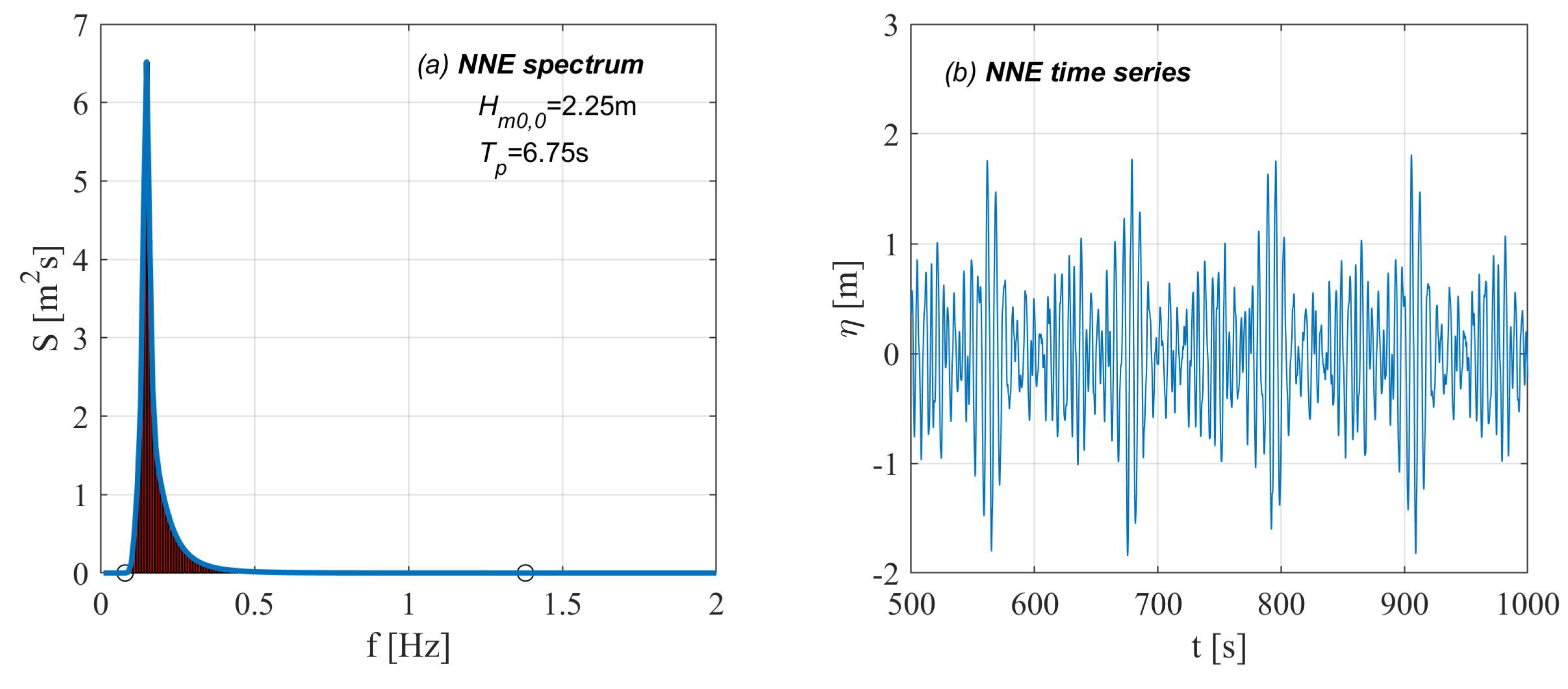
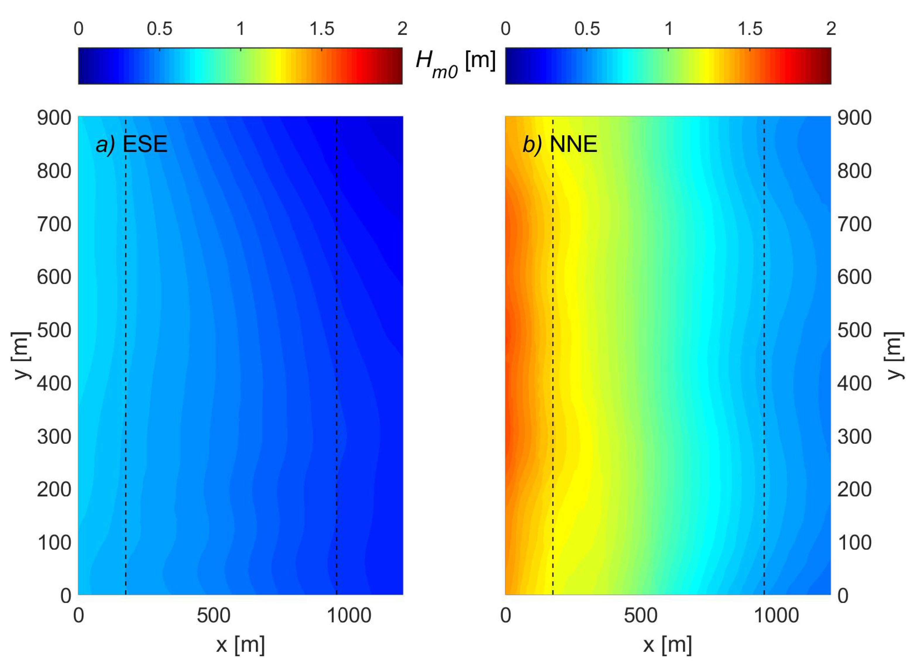
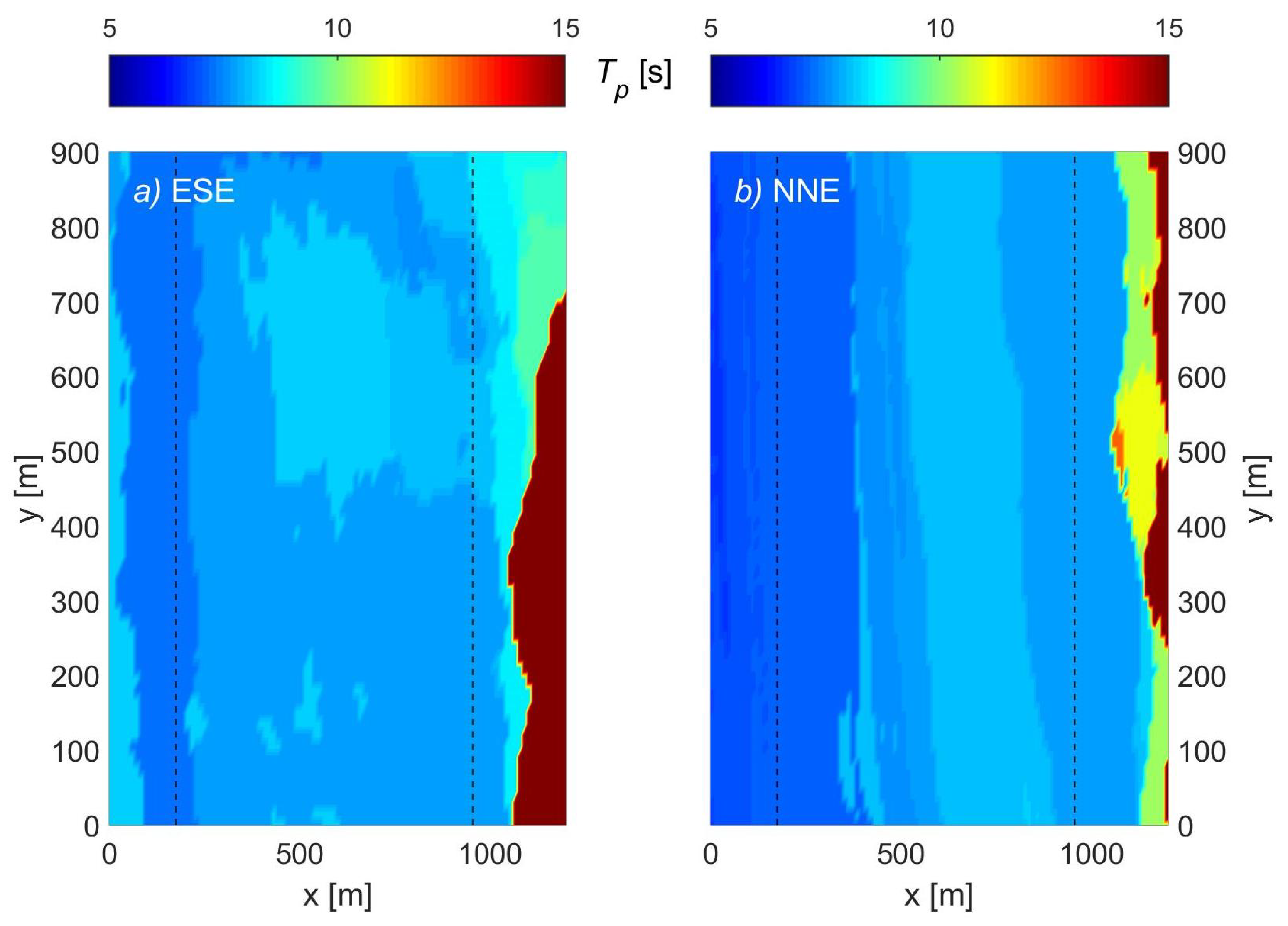
3.2. Step 2: Boundary and Initial Conditions

The estimate of the wave field is used for the generation of the boundary condition to be applied at specific locations along the cross-shore direction. In particular, simulations have been run starting from water depths of $h_{off}\approx 9$ m, located at a distance $x=175$ m from the offshore boundary, and of $h_{off}\approx 5$ m, located at $x=855$ m from the offshore boundary.

A couple of simulations has been run at each chosen depth: one characterized by the waves propagating on a surveyed beach, the other by the waves propagating on an equilibrium-profile bathymetry. While the former type of simulations reproduces the condition for which a beach survey is available, the latter type resembles the case of no availability of bathymetric data. Specifically, it has already been found that both beach inundation and runup on the emerged beach can be well reproduced if a Dean-type equilibrium profile [54] is used instead of the real beach profile. The classical equilibrium profile is expressed by the law $h=A{x}_{sh}^{2/3}$, where $x_{sh}$ is the distance to shoreline, while A is a site-specific shape parameter. Hence, a suitable equilibrium profile has been built using the following inputs: (i) the bathymetry estimate provided by the NSP method at depths $h>5$ m, (ii) a constant offshore slope of 1:200, and (iii) a constant value $A=0.065$ valid throughout the domain (in agreement with previous studies, e.g., [50]).

A total of four flood simulations associated with each baseline test have thus been run (see details in Section 3.3). These are described in Figure 8, where the top panels (a,b,c) refer to an offshore depth $h_{off}\approx 5$ m, the lower panels (d,e,f) to $h_{off}\approx 9$ m. While the left panels (a,d) illustrate the surveyed/ground-truth bathymetries, the middle panels (b,e) show the reconstructed equilibrium-profile bathymetries. The right panels (c,f) show the comparison between ground-truth (solid lines) and equilibrium (dashed lines) profiles.

The wave characteristics reconstructed using the NSP method (Section 3.1) are all reported in

Table 2. Wave characteristics used for the flood simulations.

Wave Type	Bathymetry	${\mathit{h}}_{\mathit{o}\mathit{f}\mathit{f}}$	${\mathit{H}}_{\mathit{m}0,\mathit{o}\mathit{f}\mathit{f}}$	${\mathit{T}}_{\mathit{p}}$	${\mathit{\theta }}_{0,\mathit{l}}$
		[m]	[m]	[s]	[${}^{\circ }$]
ESE	ground-truth	9.22	0.62	7.35	−17
ESE	equilibrium	9.22	0.62	7.35	−17
ESE	ground-truth	5.34	0.33	7.8	−10
ESE	equilibrium	5.34	0.33	7.8	−10
NNE	ground-truth	9.23	1.32	6.8	0
NNE	equilibrium	9.23	1.32	6.8	0
NNE	ground-truth	5.14	0.64	7.8	0
NNE	equilibrium	5.14	0.64	7.8	0

. These are used for the generation of the boundary conditions required by the flood simulations. It is worth noting that some wave heights reported in Table 2 are smaller than 1 m. Although this value represents a limit for the estimation of sea parameters in the wave-radar frame, the work by [40] showed the robustness of the NSP method for the estimation of the sea-surface current from the radar images acquired in sea conditions of “gentle breeze” with $H_{m0,off}<1$ m (level 3 on Beaufort scale), a challenging state for the X-band radar. Furthermore, the two proposed scenarios are significantly different each other, this better allowing one to evaluate the potential of the proposed methodology within a wide range of wave characteristics.

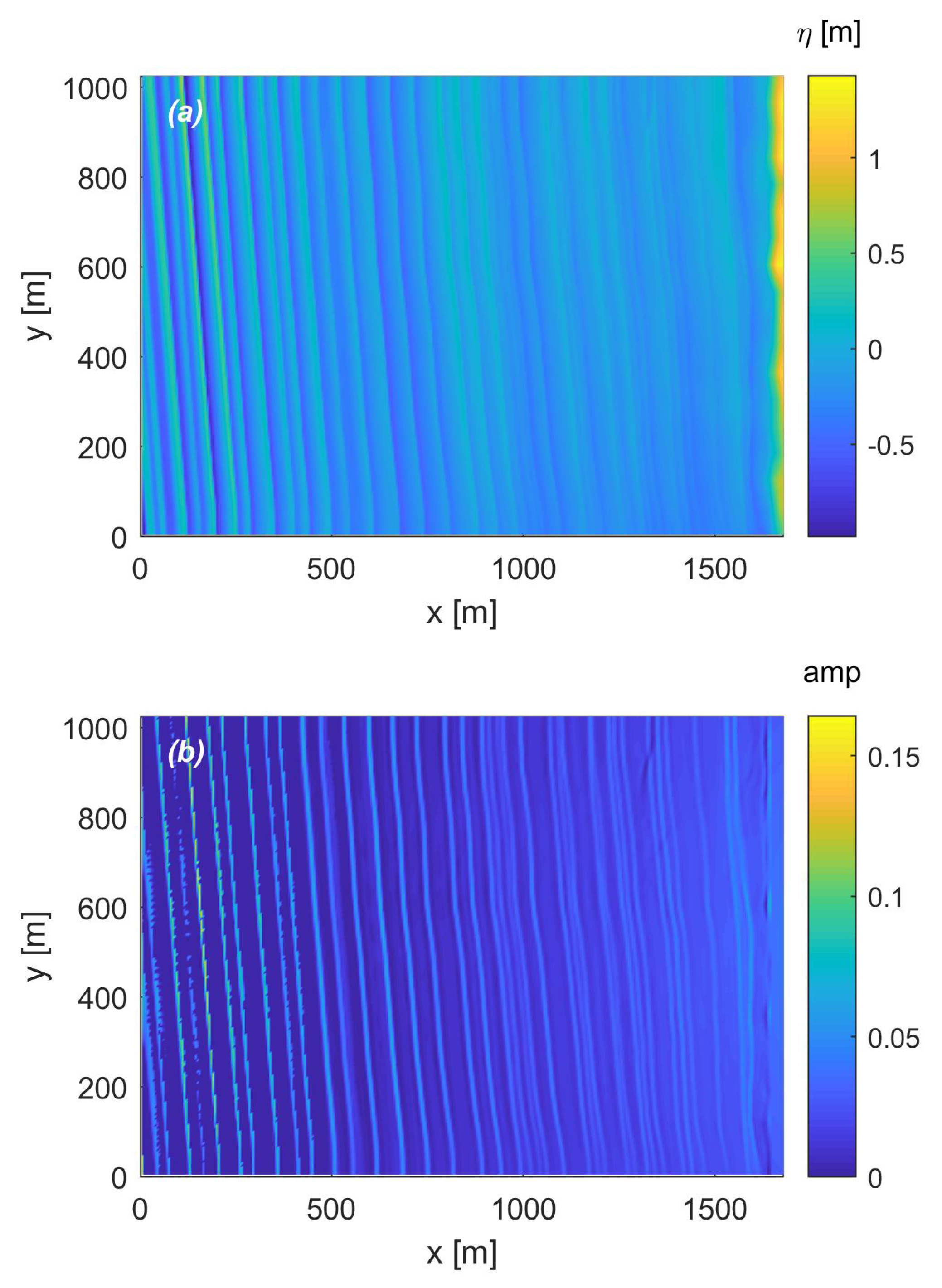
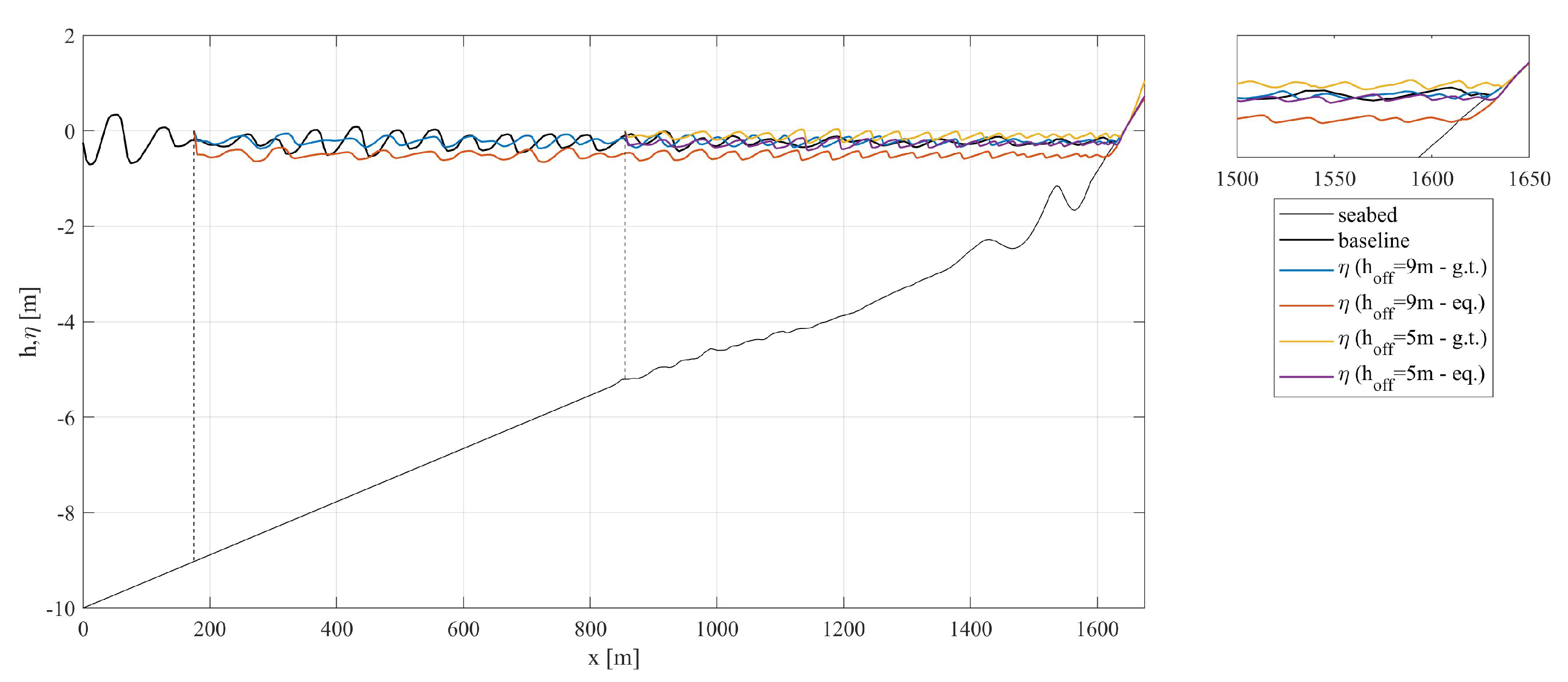
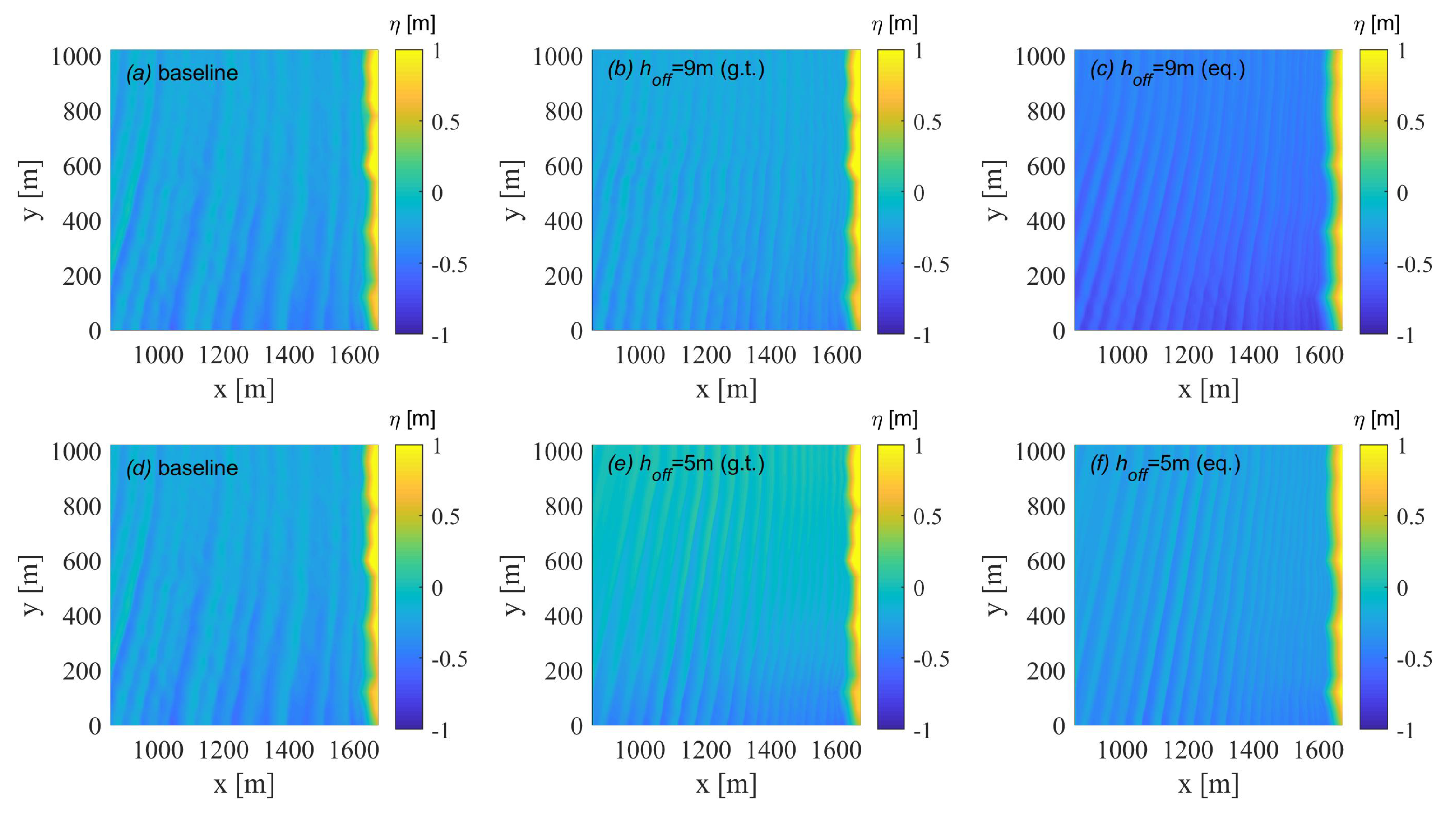
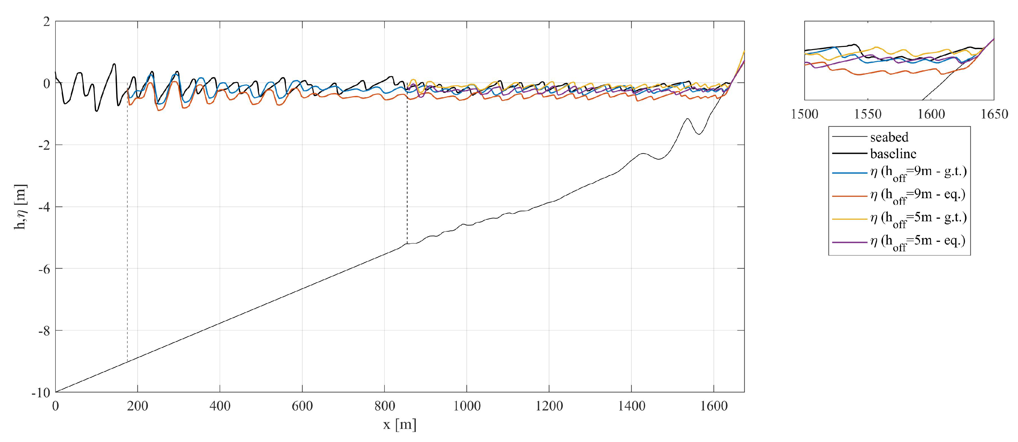
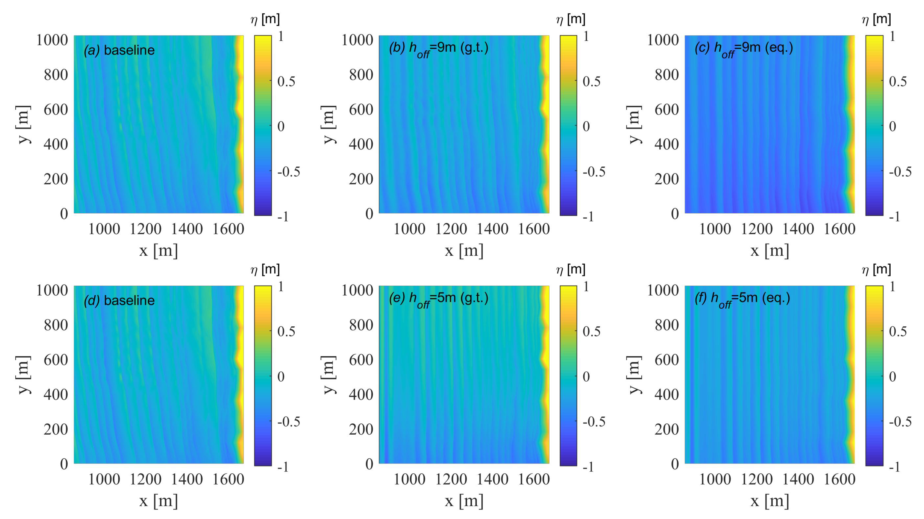
3.3. Step 3: Flood Simulations

The flood simulations have been run on the bathymetries illustrated in Figure 8 and following the prescriptions of Table 2. The water-surface elevation during the shoreward propagation of the ESE forcing, which is less steep and smaller than the NNE forcing, is illustrated in Figure 9.

During their propagation, the single waves characterizing the spectrum experience several processes, spanning from the shoaling to the breaking, the latter numerically reproduced through a water-surface discontinuity [34]. Here, the comparison between the baseline simulation (black line) and the flood-simulation (colored lines) results at time $t=1000$ s (corresponding to about 135 waves) is presented. The propagation of the wave trains, though irregular, is consistent and the order of magnitude of the free-surface elevations obtained from the different tests is the same, this being more visible from inspection of the close-up view shown in the right panel. Consistency among the simulations may also be found observing the free-surface evolution throughout the domain (Figure 10). Although some little differences can be noticed between the baseline result (left panels) and the results of the flood tests (middle and right panels), the wave propagation is the same, in terms of: wave direction from the offshore to the inshore, $\eta$ distribution, wavelength. This also in view of the random nature of the generated series.

The NNE wave, steeper and higher than the ESE, also provides good comparisons between baseline and flood simulations. Figure 11 and Figure 12 illustrate the free-surface elevation, which is a bit larger for the baseline condition compared to the flood results, e.g., at the shoreline location (see the right panel of Figure 11). The baseline wave-propagation direction (${\theta }_{0,l}=5^{\circ }$) is slightly different to that predicted, which is ${\theta }_{0,l}=0^{\circ }$, i.e., waves propagating perpendicularly to the shoreline. The sawtooth shape of the water-surface profile (Figure 11), mainly visible for the baseline simulations (black line), is due both to the wave steepening, induced by the shoaling process, and partially to the offshore displacement of the wave breaking, induced by the absence of dispersion, typical of NSWE models.

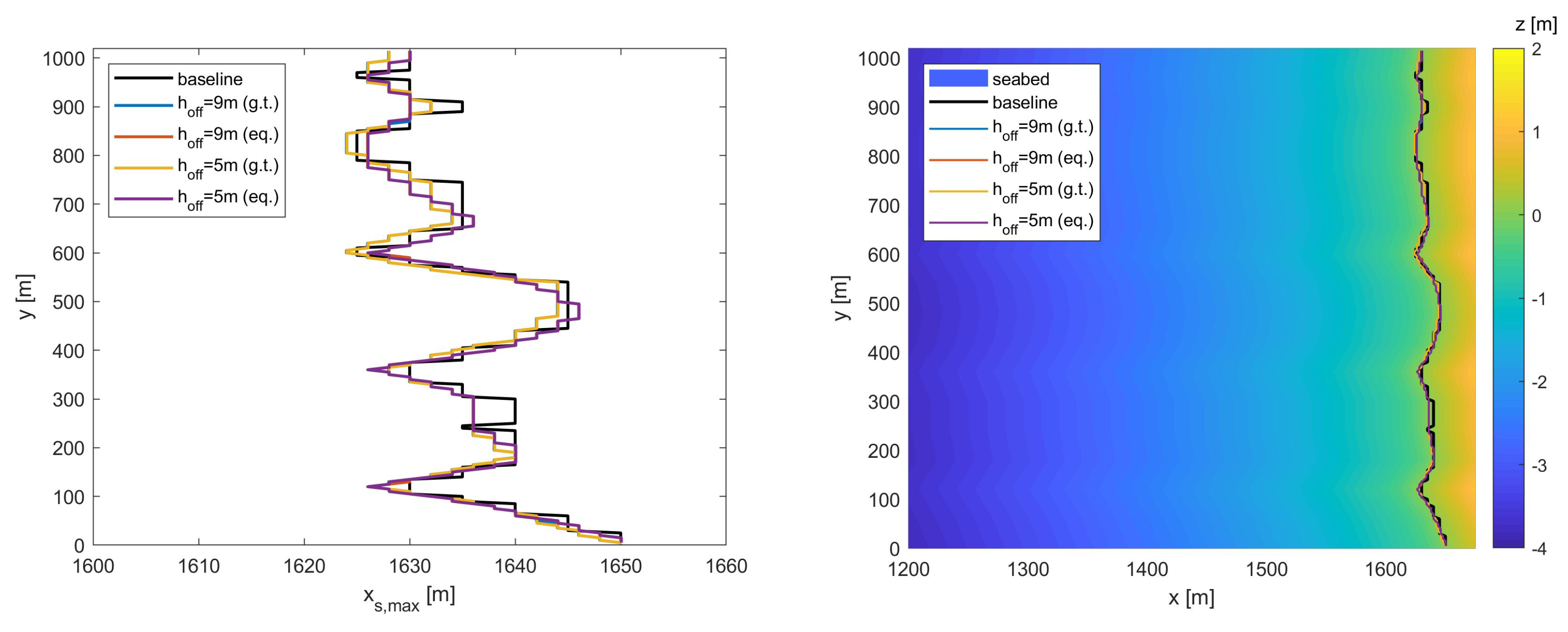
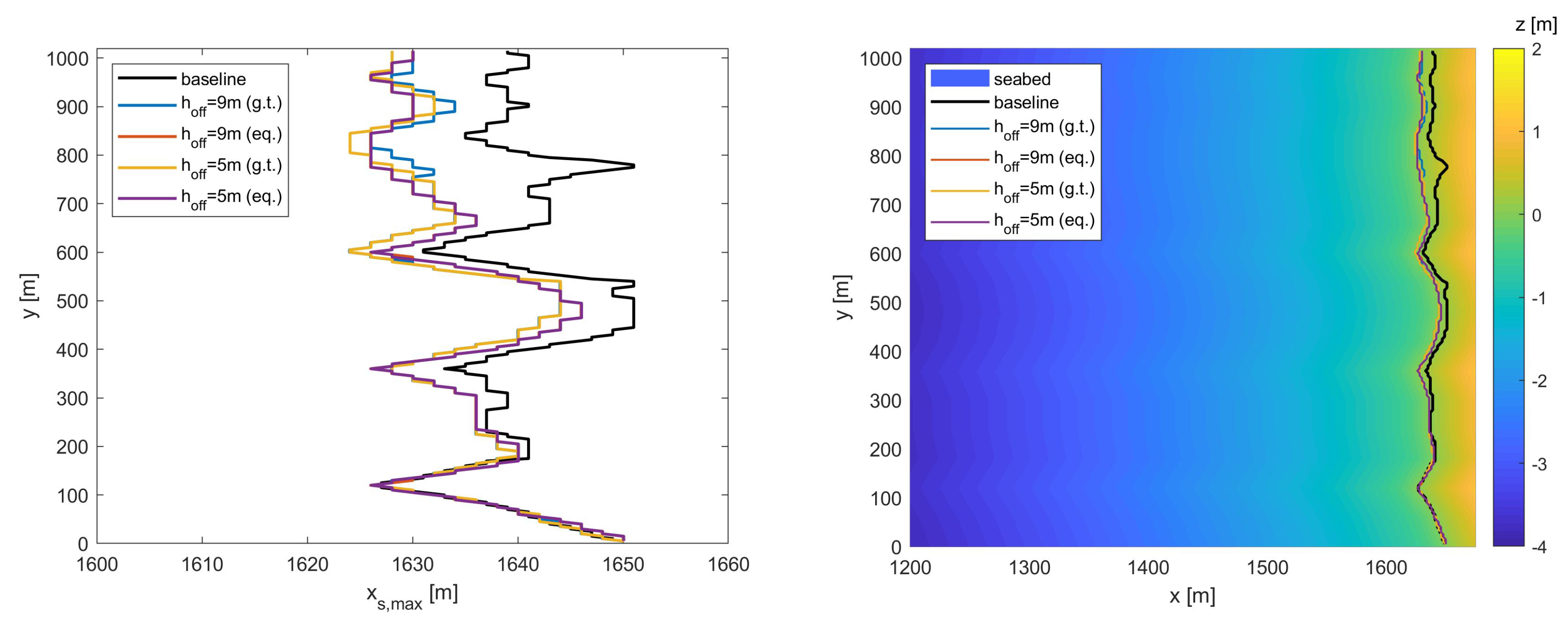
3.4. Step 4: Beach Inundation

The final step of the proposed methodology consists of the analysis of the beach inundation obtained from the different runs. The maximum shoreline location $x_{s,max}$ observed during the whole runs (test duration: 1000 s) is estimated as the envelope of the shoreline locations obtained at each time step ($\mathsf{\Delta }t=1$ s). For this purpose, every inundation line has been obtained by taking as flooded only the areas characterized by a minimum water depth $d_{flood}=10$ cm, this being consistent with risk analyses that could be undertaken on the studied zone (e.g., see [7]).

The results of the ESE simulations are illustrated in Figure 13. As can be observed, all colored lines, representing the flood simulations run using either ground-truth or equilibrium-profile beaches, are in very good agreement with the baseline simulation result (black line). These overlaps almost perfectly and the maximum distance is in the order of the grid size ($\mathsf{\Delta }x=2$ m).

The results of the NNE simulations are illustrated in Figure 14, where the beach inundation of the baseline simulation is a bit larger than that obtained from the flood simulations, which tend to slightly underestimate the flooded area. In particular, the region in the range $y=(0$–$650)$ m provides a good comparison between the two simulation types, with a maximum distance between baseline (black line) and flood-(colored lines) simulation results of 5 m. The upper region, i.e., $y=(650$–$1000)$ m, shows a weaker, though acceptable, comparison, with a maximum distance of 21 m at $y=780$ m. This may be attributed to the different propagation direction in the baseline and flood simulations (see Figure 12), due to the slight underestimate of the wave angle, i.e., ${\theta }_{0,l}=0^{\circ }$ (Table 2) versus ${\theta }_{0,l}=5^{\circ }$ (Table 1).

In summary, the RMSE values of the flood simulations with respect to the baseline test are reported in

Table 3. RMSE of the $x_{s,max}$ of the flood simulations with respect to the $x_{s,max}$ of the corresponding baseline tests.

Wave Type	Bathymetry	${\mathit{h}}_{\mathit{o}\mathit{f}\mathit{f}}$	$\mathit{R}\mathit{M}\mathit{S}\mathit{E}$
		[m]	[m]
ESE	ground-truth	9	2.28
ESE	equilibrium	9	2.34
ESE	ground-truth	5	2.26
ESE	equilibrium	5	2.34
NNE	ground-truth	9	7.67
NNE	equilibrium	9	8.07
NNE	ground-truth	5	8.40
NNE	equilibrium	5	8.05

. Errors of the order of the grid size characterize all flood simulations of the ESE case ($RMSE=(2.2$–$2.3)$ m), while acceptable values are found for the NNE case ($RMSE=(7.6$–$8.4)$ m). Such results demonstrate the suitability and robustness of the proposed methodology, which combines the use of a remote sensor with the numerical modeling for forecasting and hindcasting purposes related to the beach inundation.

4. Discussion and Conclusions

The present work aims at improving the skills of typical coastal monitoring systems. Specifically, a methodology is here illustrated based on the combination of a remote sensor (e.g., an X-band marine radar applied to the coastal environment) with a numerical model which solves the nearshore hydrodynamics (e.g., a NSWE solver).

To reach such a purpose and to suitably control the involved variables, the wave field is generated through baseline simulations aimed at reproducing wave conditions representative of the unprotected coastal area of Senigallia (Marche Region, Italy). The tilt modulation is then applied to the wave field generated through each baseline simulation to recreate a real-world radar data sequence, which can be seen as the “initial condition” of the proposed methodology.

The NSP approach is now used to reconstruct both bathymetry and wave field in the region typically covered by an X-band radar, i.e., about (1–6) km from the shoreline. It is demonstrated, here and in previous works (e.g., [31]), that the NSP is able at properly reconstructing directly some of the main variables (seabed depth, wave direction, peak wave period and significant wave height).

Such reconstructed data are then exploited for the generation of both initial and boundary conditions, to be used to feed the NSWE model. The initial condition consists of the reconstructed bathymetry (e.g., referring to seabed depths within 5 m and 9 m) which is extended up to the coast using either an existing survey or an equilibrium-profile-based bathymetry. The reconstructed wave characteristics are used to generate, following [53]’s method, the random time series of free-surface elevation, which characterizes the boundary condition of the flood simulations.

Although the end users of the proposed methodology may choose to run several simulations (e.g., based on the Monte Carlo method, to take into account the randomness of the free-surface boundary condition), the present work aims at illustrating four approaches based on two different boundary depths (around 5 m and 9 m) and two different bathymetric datasets (ground-truth and equilibrium profiles). In each simulation, the waves are propagated from the location where they are reconstructed to the coast. The beach inundation provided by flood simulations of different kinds (i.e., applying the boundary condition at a water depth of either 9 m or 5 m, rather than using either a real-world bathymetry or an equilibrium-profile-derived bathymetry) is compared to that obtained from the baseline simulations, with differences of the order of the used grid size. Better results are those retrieved when a milder forcing, coming from ESE, is used, while steeper and higher waves, coming from NNE, provide a slightly weaker comparison, likely induced by a slight underestimate of the wave direction.

Finally, the present work demonstrates that a suitable coupling between NSP approach and numerical simulations leads to good results in terms of coastal flooding in real-world environments. This can provide useful information for the coastal environment and the related stakeholders (coast authorities, municipalities, beach resort owners, etc.), mainly dealing with: (i) real-time predictions of coastal flooding and warning systems; (ii) hazard mapping and coastal risk analysis; (iii) integrated coastal zone management.

A real-world application of the proposed methodology is expected in the near future, based on the NSP application to a radar data sequence, combined to depth-averaged/shallow-water simulations.

References

1. CCCuk. UK Climate Change Risk Assessment 2017. Synthesis report: Priorities for the next five years. In UK Climate Change Risk Assessment 2017 Synthesis Report of Committee on Climate Change; Technical Report; CCCuk: London, UK, 2016. [Google Scholar]
2. Barcikowska, M.J.; Weaver, S.J.; Feser, F.; Russo, S.; Schenk, F.; Stone, D.A.; Wehner, M.F.; Zahn, M. Euro-Atlantic winter storminess and precipitation extremes under 1.5 C vs. 2 C warming scenarios. Earth Syst. Dyn. 2018, 9, 679–699. [Google Scholar] [CrossRef]
3. Lin, N.; Emanuel, K.A.; Smith, J.A.; Vanmarcke, E. Risk assessment of hurricane storm surge for New York City. J. Geophys. Res. Atmos. 2010, 115. [Google Scholar] [CrossRef] [Green Version]
4. Bosom García, E.; Jiménez Quintana, J.A. Probabilistic coastal vulnerability assessment to storms at regional scale: application to Catalan beaches (NW Mediterranean). Nat. Hazards Earth Syst. Sci. 2011, 11, 475–484. [Google Scholar] [CrossRef]
5. Perini, L.; Calabrese, L.; Salerno, G.; Ciavola, P.; Armaroli, C. Evaluation of coastal vulnerability to flooding: comparison of two different methodologies adopted by the Emilia-Romagna region (Italy). Nat. Hazards Earth Syst. Sci. 2016, 16, 181–194. [Google Scholar] [CrossRef] [Green Version]
6. Leo, F.D.; Besio, G.; Zolezzi, G.; Bezzi, M. Coastal vulnerability assessment: through regional to local downscaling of wave characteristics along the Bay of Lalzit (Albania). Nat. Hazards Earth Syst. Sci. 2019, 19, 287–298. [Google Scholar] [CrossRef] [Green Version]
7. Postacchini, M.; Lalli, F.; Memmola, F.; Bruschi, A.; Bellafiore, D.; Lisi, I.; Zitti, G.; Brocchini, M. A model chain approach for coastal inundation: Application to the bay of Alghero. Estuar. Coast. Shelf Sci. 2019, 219, 56–70. [Google Scholar] [CrossRef]
8. Neumann, B.; Vafeidis, A.T.; Zimmermann, J.; Nicholls, R.J. Future coastal population growth and exposure to sea-level rise and coastal flooding—A global assessment. PLoS ONE 2015, 10, e0118571. [Google Scholar] [CrossRef] [PubMed]
9. UNEP/MAP. Protocol on Integrated Coastal Zone Management in the Mediterranean; Technical Report; UNEP/MAP: Nairobi, Kenya, 2008. [Google Scholar]
10. Rochette, J.; Bille, R. ICZM protocols to regional seas conventions: What? why? how? Mar. Policy 2012, 36, 977–984. [Google Scholar] [CrossRef]
11. Ernoul, L.; Wardell-Johnson, A. Environmental discourses: Understanding the implications on ICZM protocol implementation in two Mediterranean deltas. Ocean Coast. Manag. 2015, 103, 97–108. [Google Scholar] [CrossRef]
12. Herbers, T.; Jessen, P.; Janssen, T.; Colbert, D.; MacMahan, J. Observing ocean surface waves with GPS-tracked buoys. J. Atmos. Ocean. Technol. 2012, 29, 944–959. [Google Scholar] [CrossRef]
13. Ohlmann, J.C.; Fewings, M.R.; Melton, C. Lagrangian observations of inner-shelf motions in Southern California: Can surface waves decelerate shoreward-moving drifters just outside the surf zone? J. Phys. Oceanogr. 2012, 42, 1313–1326. [Google Scholar] [CrossRef]
14. Rogers, W.E.; Holland, K.T. A study of dissipation of wind-waves by mud at Cassino Beach, Brazil: Prediction and inversion. Cont. Shelf Res. 2009, 29, 676–690. [Google Scholar] [CrossRef]
15. Brocchini, M.; Calantoni, J.; Postacchini, M.; Sheremet, A.; Staples, T.; Smith, J.; Reed, A.H.; Braithwaite, E.F., III; Lorenzoni, C.; Russo, A.; et al. Comparison between the wintertime and summertime dynamics of the Misa River estuary. Mar. Geol. 2017, 385, 27–40. [Google Scholar] [CrossRef] [Green Version]
16. Melville, W.; Loewen, M.R.; Felizardo, F.C.; Jessup, A.T.; Buckingham, M. Acoustic and microwave signatures of breaking waves. Nature 1988, 336, 54. [Google Scholar] [CrossRef]
17. Nieto Borge, J.; RodrÍguez, G.R.; Hessner, K.; González, P.I. Inversion of marine radar images for surface wave analysis. J. Atmos. Ocean. Technol. 2004, 21, 1291–1300. [Google Scholar] [CrossRef]
18. Archetti, R.; Paci, A.; Carniel, S.; Bonaldo, D. Optimal index related to the shoreline dynamics during a storm: The case of Jesolo beach. Nat. Hazards Earth Syst. Sci. 2016, 16, 1107–1122. [Google Scholar] [CrossRef]
19. Benetazzo, A.; Serafino, F.; Bergamasco, F.; Ludeno, G.; Ardhuin, F.; Sutherland, P.; Sclavo, M.; Barbariol, F. Stereo imaging and X-band radar wave data fusion: An assessment. Ocean Eng. 2018, 152, 346–352. [Google Scholar] [CrossRef] [Green Version]
20. Díaz, H.; Catalán, P.; Wilson, G. Quantification of Two-Dimensional Wave Breaking Dissipation in the Surf Zone from Remote Sensing Data. Remote Sens. 2018, 10, 38. [Google Scholar]
21. Bell, P.S.; Osler, J.C. Mapping bathymetry using X-band marine radar data recorded from a moving vessel. Ocean Dyn. 2011, 61, 2141–2156. [Google Scholar] [CrossRef]
22. Ludeno, G.; Orlandi, A.; Lugni, C.; Brandini, C.; Soldovieri, F.; Serafino, F. X-band marine radar system for high-speed navigation purposes: A test case on a cruise ship. IEEE Geosci. Remote Sens. Lett. 2014, 11, 244–248. [Google Scholar] [CrossRef]
23. Lund, B.; Graber, H.C.; Hessner, K.; Williams, N.J. On shipboard marine X-band radar near-surface current “calibration”. J. Atmos. Ocean. Technol. 2015, 32, 1928–1944. [Google Scholar] [CrossRef]
24. Ludeno, G.; Brandini, C.; Lugni, C.; Arturi, D.; Natale, A.; Soldovieri, F.; Gozzini, B.; Serafino, F. Remocean system for the detection of the reflected waves from the costa concordia ship wreck. IEEE J. Sel. Top. Appl. Earth Obs. Remote Sens. 2014, 7, 3011–3018. [Google Scholar] [CrossRef]
25. Ludeno, G.; Reale, F.; Dentale, F.; Carratelli, E.; Natale, A.; Soldovieri, F.; Serafino, F. An X-band radar system for bathymetry and wave field analysis in a harbour area. Sensors 2015, 15, 1691–1707. [Google Scholar] [CrossRef] [PubMed]
26. Gangeskar, R. Ocean current estimated from X-band radar sea surface, images. IEEE Trans. Geosci. Remote Sens. 2002, 40, 783–792. [Google Scholar] [CrossRef]
27. Senet, C.M.; Seemann, J.; Flampouris, S.; Ziemer, F. Determination of bathymetric and current maps by the method DiSC based on the analysis of nautical X-band radar image sequences of the sea surface (November 2007). IEEE Trans. Geosci. Remote Sens. 2008, 46, 2267–2279. [Google Scholar] [CrossRef]
28. Young, I.R.; Rosenthal, W.; Ziemer, F. A three-dimensional analysis of marine radar images for the determination of ocean wave directionality and surface currents. J. Geophys. Res. Oceans 1985, 90, 1049–1059. [Google Scholar] [CrossRef] [Green Version]
29. Senet, C.M.; Seemann, J.; Ziemer, F. The near-surface current velocity determined from image sequences of the sea surface. IEEE Trans. Geosci. Remote Sens. 2001, 39, 492–505. [Google Scholar] [CrossRef]
30. Serafino, F.; Lugni, C.; Soldovieri, F. A novel strategy for the surface current determination from marine X-band radar data. IEEE Geosci. Remote Sens. Lett. 2010, 7, 231–235. [Google Scholar] [CrossRef]
31. Ludeno, G.; Postacchini, M.; Natale, A.; Brocchini, M.; Lugni, C.; Soldovieri, F.; Serafino, F. Normalized Scalar Product Approach for Nearshore Bathymetric Estimation From X-Band Radar Images: An Assessment Based on Simulated and Measured Data. IEEE J. Ocean. Eng. 2018, 43, 221–237. [Google Scholar] [CrossRef]
32. Bellafiore, D.; Zaggia, L.; Broglia, R.; Ferrarin, C.; Barbariol, F.; Zaghi, S.; Lorenzetti, G.; Manfè, G.; De Pascalis, F.; Benetazzo, A. Modeling ship-induced waves in shallow water systems: The Venice experiment. Ocean Eng. 2018, 155, 227–239. [Google Scholar] [CrossRef]
33. Gaeta, M.; Bonaldo, D.; Samaras, A.; Carniel, S.; Archetti, R. Coupled Wave-2D Hydrodynamics Modeling at the Reno River Mouth (Italy) under Climate Change Scenarios. Water 2018, 10, 1380. [Google Scholar] [CrossRef]
34. Brocchini, M.; Bernetti, R.; Mancinelli, A.; Albertini, G. An efficient solver for nearshore flows based on the WAF method. Coast. Eng. 2001, 43, 105–129. [Google Scholar] [CrossRef]
35. Briganti, R.; Torres-Freyermuth, A.; Baldock, T.E.; Brocchini, M.; Dodd, N.; Hsu, T.J.; Jiang, Z.; Kim, Y.; Pintado-Patiño, J.C.; Postacchini, M. Advances in numerical modelling of swash zone dynamics. Coast. Eng. 2016, 115, 26–41. [Google Scholar] [CrossRef]
36. Kennedy, A.B.; Chen, Q.; Kirby, J.T.; Dalrymple, R.A. Boussinesq modeling of wave transformation, breaking, and runup. I: 1D. J. Waterw. Port Coast. Ocean Eng. 2000, 126, 39–47. [Google Scholar] [CrossRef]
37. Antuono, M.; Colicchio, G.; Lugni, C.; Greco, M.; Brocchini, M. A depth semi-averaged model for coastal dynamics. Phys. Fluids 2017, 29, 056603. [Google Scholar] [CrossRef] [Green Version]
38. Tonelli, M.; Petti, M. Hybrid finite volume—Finite difference scheme for 2DH improved Boussinesq equations. Coast. Eng. 2009, 56, 609–620. [Google Scholar] [CrossRef]
39. Shi, F.; Kirby, J.T.; Harris, J.C.; Geiman, J.D.; Grilli, S.T. A high-order adaptive time-stepping TVD solver for Boussinesq modeling of breaking waves and coastal inundation. Ocean Model. 2012, 43, 36–51. [Google Scholar] [CrossRef]
40. Ludeno, G.; Nasello, C.; Raffa, F.; Ciraolo, G.; Soldovieri, F.; Serafino, F. A comparison between drifter and X-band wave radar for sea surface current estimation. Remote Sens. 2016, 8, 695. [Google Scholar] [CrossRef]
41. Plant, W. Studies of backscattered sea return with a CW, dual-frequency, X-band radar. IEEE J. Ocean. Eng. 1977, 2, 28–36. [Google Scholar] [CrossRef]
42. Lee, P.; Barter, J.; Beach, K.; Hindman, C.; Lake, B.; Rungaldier, H.; Shelton, J.; Williams, A.; Yee, R.; Yuen, H. X band microwave backscattering from ocean waves. J. Geophys. Res. Oceans 1995, 100, 2591–2611. [Google Scholar] [CrossRef]
43. Wetzel, L.B. Electromagnetic scattering from the sea at low grazing angles. In Surface Waves and Fluxes; Springer: Dordrecht, The Netherlands, 1990; pp. 109–171. [Google Scholar]
44. Hessner, K.; Reichert, K.; Borge, J.C.N.; Stevens, C.L.; Smith, M.J. High-resolution X-band radar measurements of currents, bathymetry and sea state in highly inhomogeneous coastal areas. Ocean Dyn. 2014, 64, 989–998. [Google Scholar] [CrossRef]
45. Ludeno, G.; Flampouris, S.; Lugni, C.; Soldovieri, F.; Serafino, F. A novel approach based on marine radar data analysis for high-resolution bathymetry map generation. IEEE Geosci. Remote Sens. Lett. 2014, 11, 234–238. [Google Scholar] [CrossRef]
46. Raffa, F.; Ludeno, G.; Patti, B.; Soldovieri, F.; Mazzola, S.; Serafino, F. X-band wave radar for coastal upwelling detection off the southern coast of Sicily. J. Atmos. Ocean. Technol. 2017, 34, 21–31. [Google Scholar] [CrossRef]
47. Lund, B.; Collins, C.O.; Graber, H.C.; Terrill, E.; Herbers, T.H. Marine radar ocean wave retrieval’s dependency on range and azimuth. Ocean Dyn. 2014, 64, 999–1018. [Google Scholar] [CrossRef]
48. Kriebel, D.L.; Dean, R.G. Convolution method for time-dependent beach-profile response. J. Waterw. Port Coast. Ocean Eng. 1993, 119, 204–226. [Google Scholar] [CrossRef]
49. Soldini, L.; Antuono, M.; Brocchini, M. Numerical modeling of the influence of the beach profile on wave run-up. J. Waterw. Port Coast. Ocean Eng. 2013, 139, 61–71. [Google Scholar] [CrossRef]
50. Postacchini, M.; Soldini, L.; Lorenzoni, C.; Mancinelli, A. Medium-term dynamics of a middle Adriatic barred beach. Ocean Sci. 2017, 13, 719. [Google Scholar] [CrossRef]
51. Parlagreco, L.; Melito, L.; Devoti, S.; Perugini, E.; Soldini, L.; Zitti, G.; Brocchini, M. Monitoring for Coastal Resilience: Preliminary Data from Five Italian Sandy Beaches. Sensors 2019, 19, 1854. [Google Scholar] [CrossRef]
52. Melito, L.; Postacchini, M.; Sheremet, A.; Calantoni, J.; Zitti, G.; Darvini, G.; Brocchini, M. Hydrodynamics at a Microtidal Inlet: Analysis of Propagation of the Main Wave Components. Estuar. Coast. Shelf Sci. 2019. under review. [Google Scholar]
53. Liu, Z.; Frigaard, P. Generation and Analysis of Random Waves; Technical Report; Aalborg Universitet: Aalborg, Denmark, 1990. [Google Scholar]
54. Dean, R.G. Equilibrium beach profiles: Characteristics and applications. J. Coast. Res. 1991, 7, 53–84. [Google Scholar]
Figure 1. Sketch of the methodology applied in the present work (left) or to be applied to the real world (right).
Jmse 07 00325 g001
Figure 2. Original ground-truth bathymetry used for the baseline simulations.
Jmse 07 00325 g002
Figure 3. Example of the offshore boundary condition generation: (a) spectrum of the NNE wave; (b) surface-level time series.
Jmse 07 00325 g003
Figure 4. (a) Synthetic sea-wave image obtained from the NSWE solver. (b) Simulated radar image.
Jmse 07 00325 g004
Figure 5. Reconstructed bathymetries: (a) ESE and (b) NNE simulations. Dashed lines indicate the locations at which the boundary conditions are chosen.
Jmse 07 00325 g005
Figure 6. Reconstructed significant wave height: (a) ESE and (b) NNE simulations. Dashed lines indicate the locations at which the boundary conditions are chosen.
Jmse 07 00325 g006
Figure 7. Reconstructed peak periods: (a) ESE and (b) NNE simulations. Dashed lines indicate the locations at which the boundary conditions are chosen.
Jmse 07 00325 g007
Figure 8. Ground-truth bathymetries (a,d) and equilibrium-profile-based bathymetries (b,e) relevant to an offshore depth of 5 m (top panels) and 9 m (bottom panels). Comparisons between ground-truth and equilibrium profiles is also illustrated (c,f).
Jmse 07 00325 g008
Figure 9. Cross-section of free-surface level at t = 1000 s (∼135 waves) for the ESE tests: baseline simulation (black thick line) vs. flood simulations (colored lines). The starting points of the flood simulations, corrsponding to h 9 m and h 5 m, are also illustrated (vertical dashed lines). The little right panel shows a close-up view in the shallowest region.
Jmse 07 00325 g009
Figure 10. Free-surface level at t = 1000 s (∼135 waves) for the ESE tests: baseline simulation (a,d), flood simulations with boundary condition at h 9 m (b,c) and at h 5 m (e,f). Ground-truth-based (b,d) and equilibrium-based (c,f) tests.
Jmse 07 00325 g010
Figure 11. Cross-section of free-surface level at t = 1000 s (∼135 waves) for the NNE tests: baseline simulation (black thick line) vs. flood simulations (colored lines). The starting points of the flood simulations, corresponding to h 9 m and h 5 m, are also illustrated (vertical dashed lines). The little right panel shows a close-up view in the shallowest region.
Jmse 07 00325 g011
Figure 12. Free-surface level at t = 1000 s (∼135 waves) for the NNE tests: baseline simulation (a,d), flood simulations with boundary condition at h 9 m (b,c) and at h 5 m (e,f). Ground-truth-based (b,d) and equilibrium-based (c,f) tests.
Jmse 07 00325 g012
Figure 13. Comparison of max inundation due to the ESE forcing: results of baseline (black line) and flood (colored lines) simulations (left panel). The overlap with the original bathymetry is also shown (right panel).
Jmse 07 00325 g013
Figure 14. Comparison of max inundation due to the NNE forcing: results of baseline (black line) and flood (colored lines) simulations (left panel). The overlap with the original bathymetry is also shown (right panel).
Jmse 07 00325 g014