Numerical Modelling of a Mussel Line System by Means of Lumped-Mass Approach


Abstract
:1. Introduction
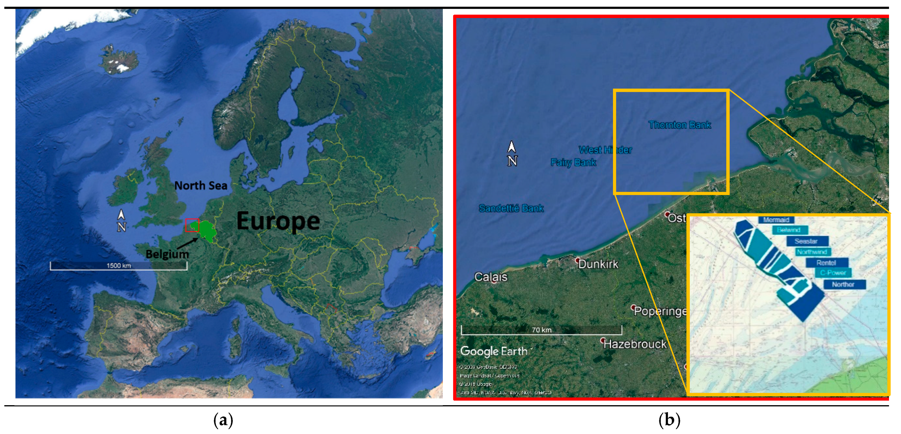
2. Field Site
3. Methodology
3.1. General Description of Numerical Models: MoorDyn
- Fixed: Fixed type restricts the node to prevent any displacement in position.
- Vessel: This type only allows the node to move according to a prescribed motion provided as an input to the code. External forces do not influence the displacement of vessel type connection nodes.
- Connect: This type allows the node to freely move in any directions according to all the forces acting on it.
3.2. Mathematical Model
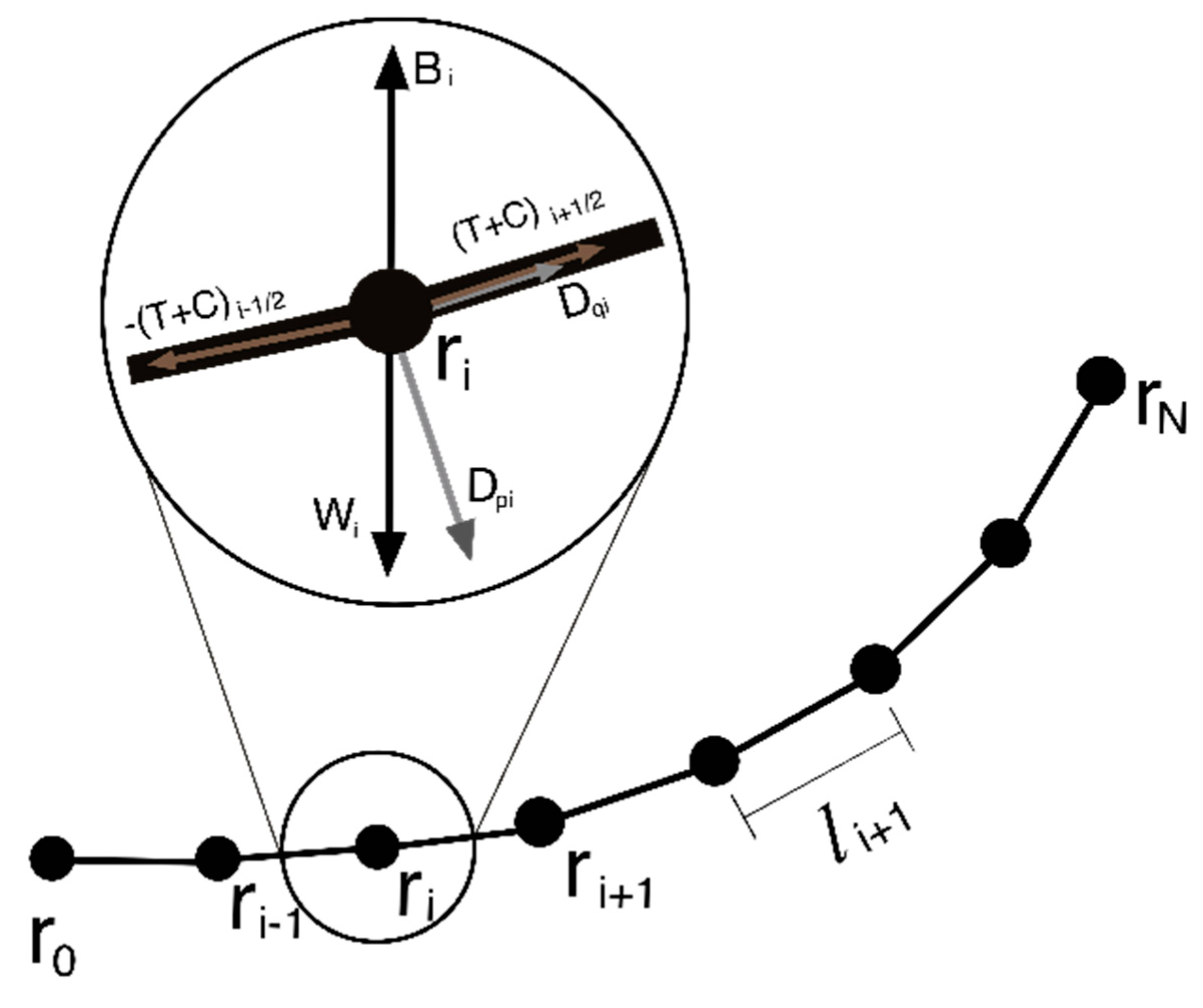
3.2.1. Equation of Motion
- is the node’s position at instantaneous time t [m];
- is the node’s velocity at instantaneous time t [m/s];
- is the node’s acceleration at instantaneous time t [m/s2];
- i represents the 3 degree of freedom in translation (i = 1, 2, 3);
- is the fluid velocity at instantaneous time t [m/s];
- is the fluid acceleration at instantaneous time t [m/s2];
- is the mass of the node [kg];
- is the hydrodynamic added mass of the node [kg];
- is the total force acting on the node [N].
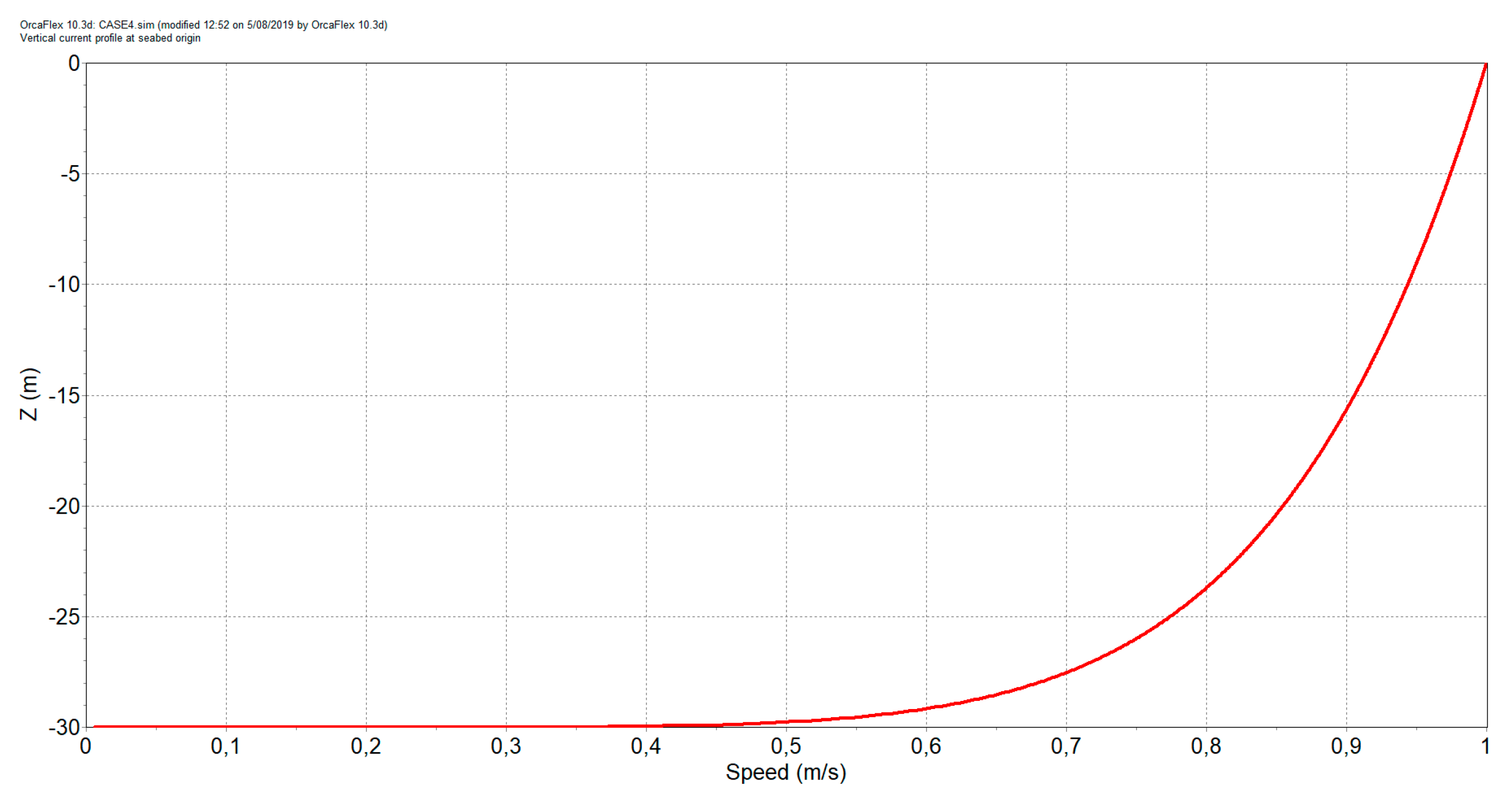
3.2.2. Current
- is the current magnitude at a reference depth (defined in the input) [m/s];
- d is the water depth (defined in the input) [m];
- is the reference depth (defined in the input) [m];
- is the exponent to control the shape of vertical distribution [-];
- is the current velocity component in x-direction [m/s];
- is the current velocity component in y-direction [m/s];
- is the current velocity component in z-direction [m/s].
3.2.3. Waves
- is the free surface elevation [m];
- is the number of wave frequency [-];
- is the number of wave direction [-];
- is the wave amplitude [m];
- is the wave angular frequency [rad/s];
- is the instantaneous time [s];
- is the wavenumber [rad/m];
- is the water depth [m];
- is the wave direction [rad];
- is the phase angle [rad];
- is the wave-induced velocity component in x-direction [m/s];
- is the wave-induced velocity component in y-direction [m/s];
- is the wave-induced velocity component in z-direction [m/s];
- is the wave-induced acceleration component x-direction [m/s2];
- is the wave-induced acceleration component y-direction [m/];
- is the wave-induced acceleration component z-direction [m/s2].
3.2.4. Wave-Current Interaction
3.2.5. Hydrodynamic Forces
- is the drag coefficient [-];
- is the inertia coefficient [-];
- is the cylinder equivalent diameter [m];
- is the density of the water [kg/m].
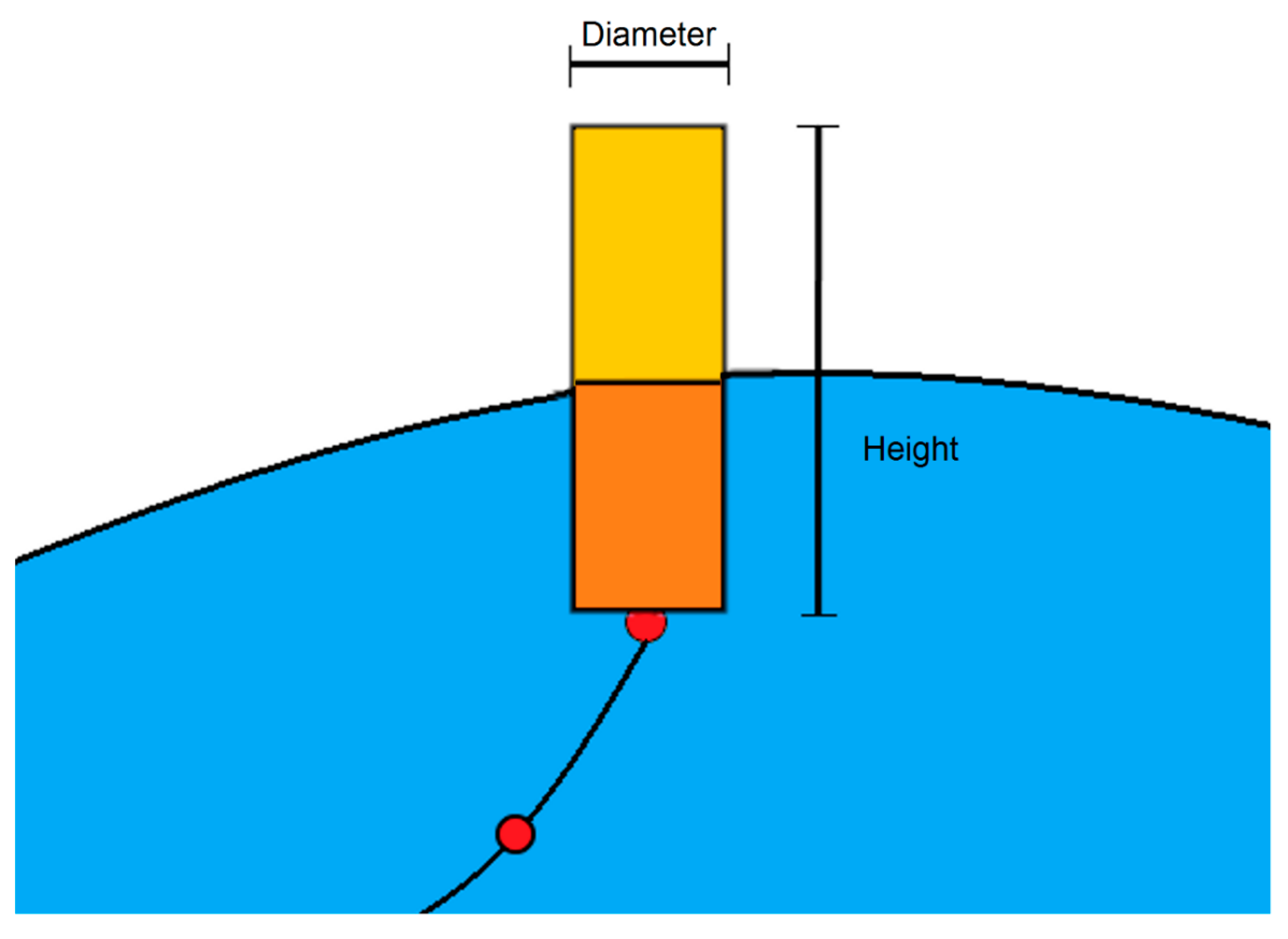
3.2.6. Buoys and Clump Weights
3.2.7. Seabed Friction
3.3. Adapted MoorDyn and OrcaFlex Comparison
3.3.1. Seabed Friction
3.3.2. Line Theory
- is the effective tension;
- is the wall tension;
- , are the internal and external pressure;
- , are the internal and external cross-section stress area;
- is the axial stiffness of the line, which is Young’s modulus multiple by cross-section area;
- is the instantaneous length of the segment;
- is the strain;
- is the segment’s unstretched length;
- is Poisson ration;
- is tension and torque coupling;
- is the segment twist angle;
- is damping coefficient;
- is the rate of increase of length.
3.3.3. Waves
3.3.4. Integration Scheme
3.4. Test Cases Setup
3.5. Environmental Loads
4. Results and Discussions
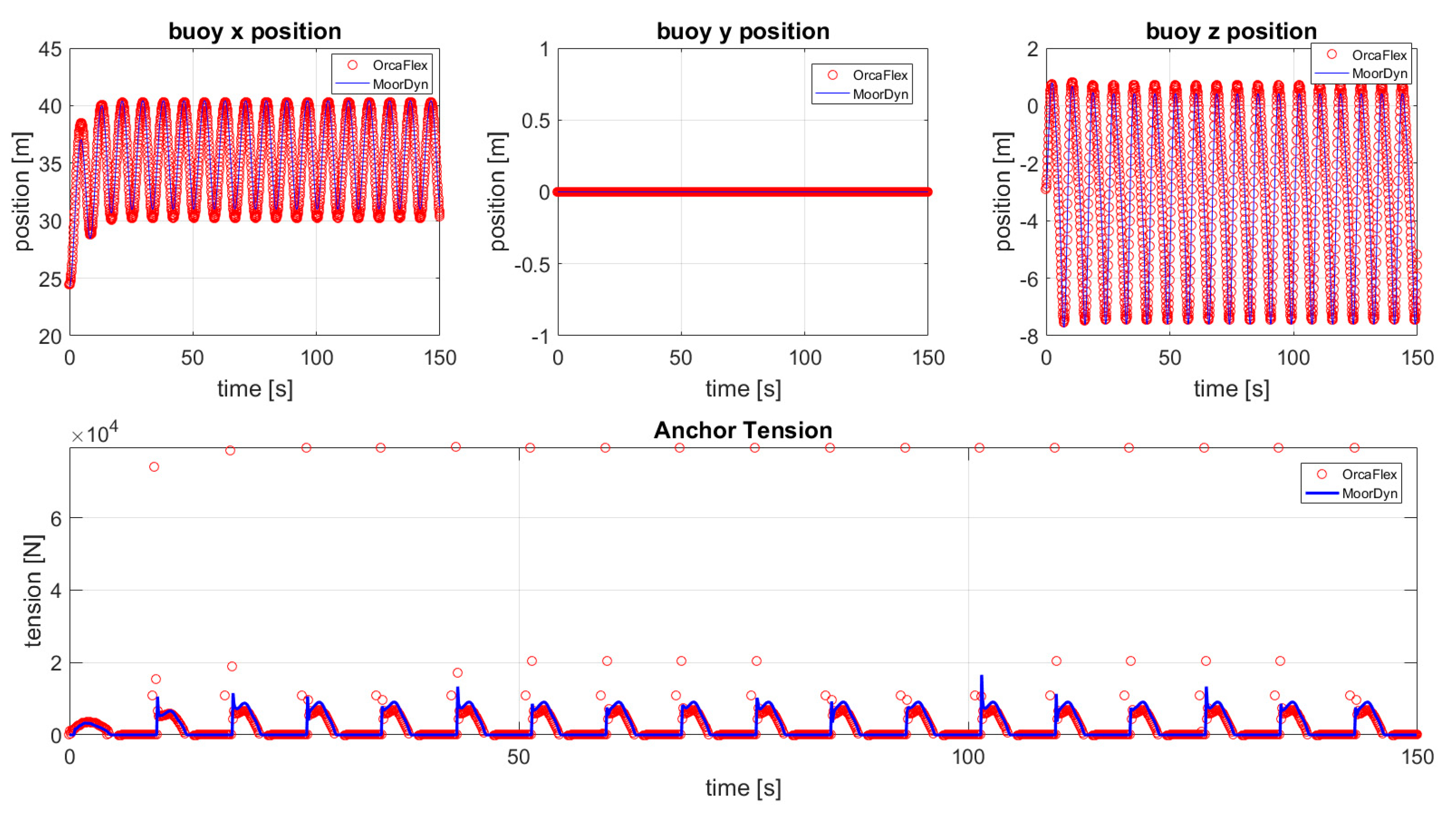
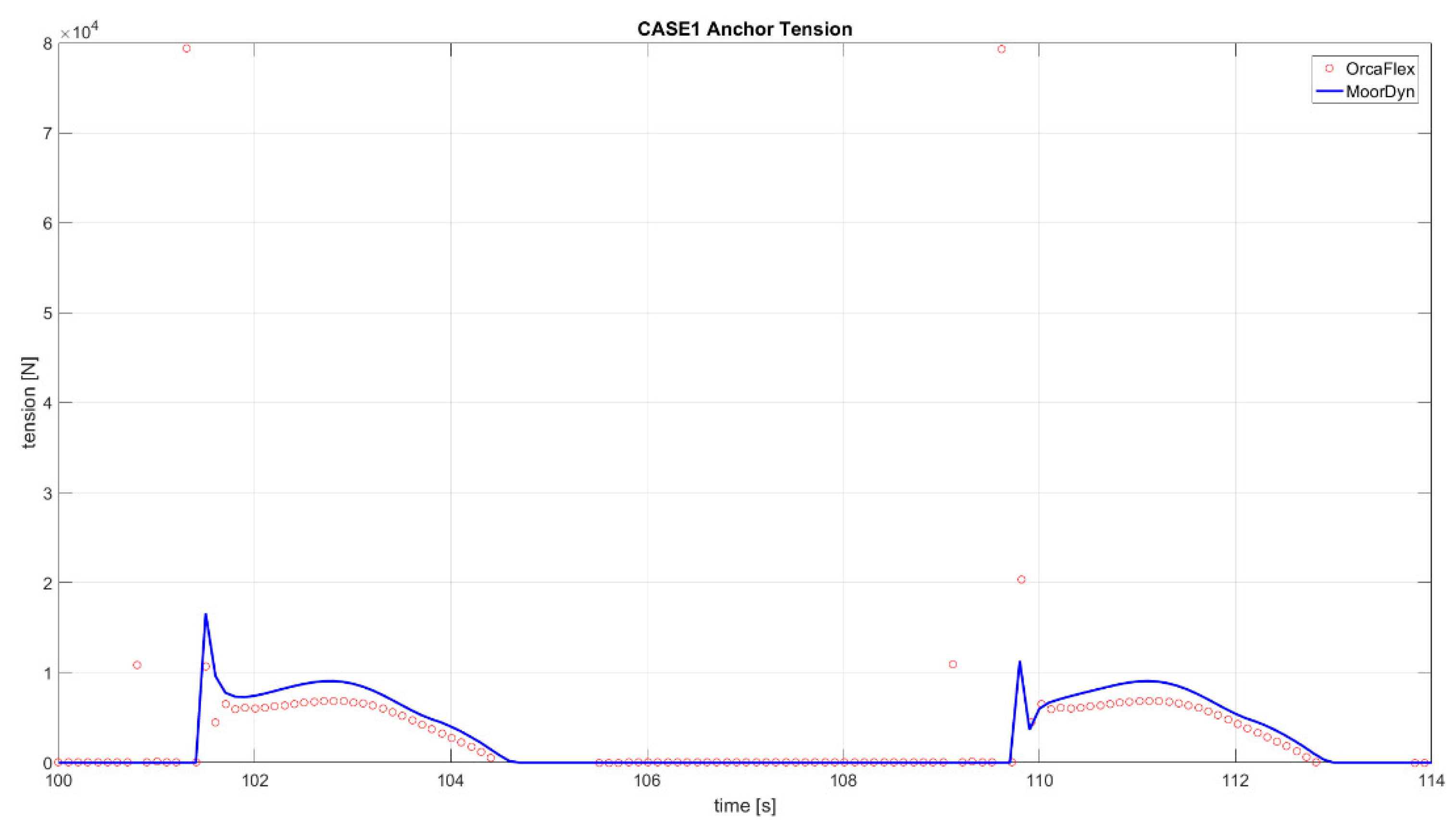
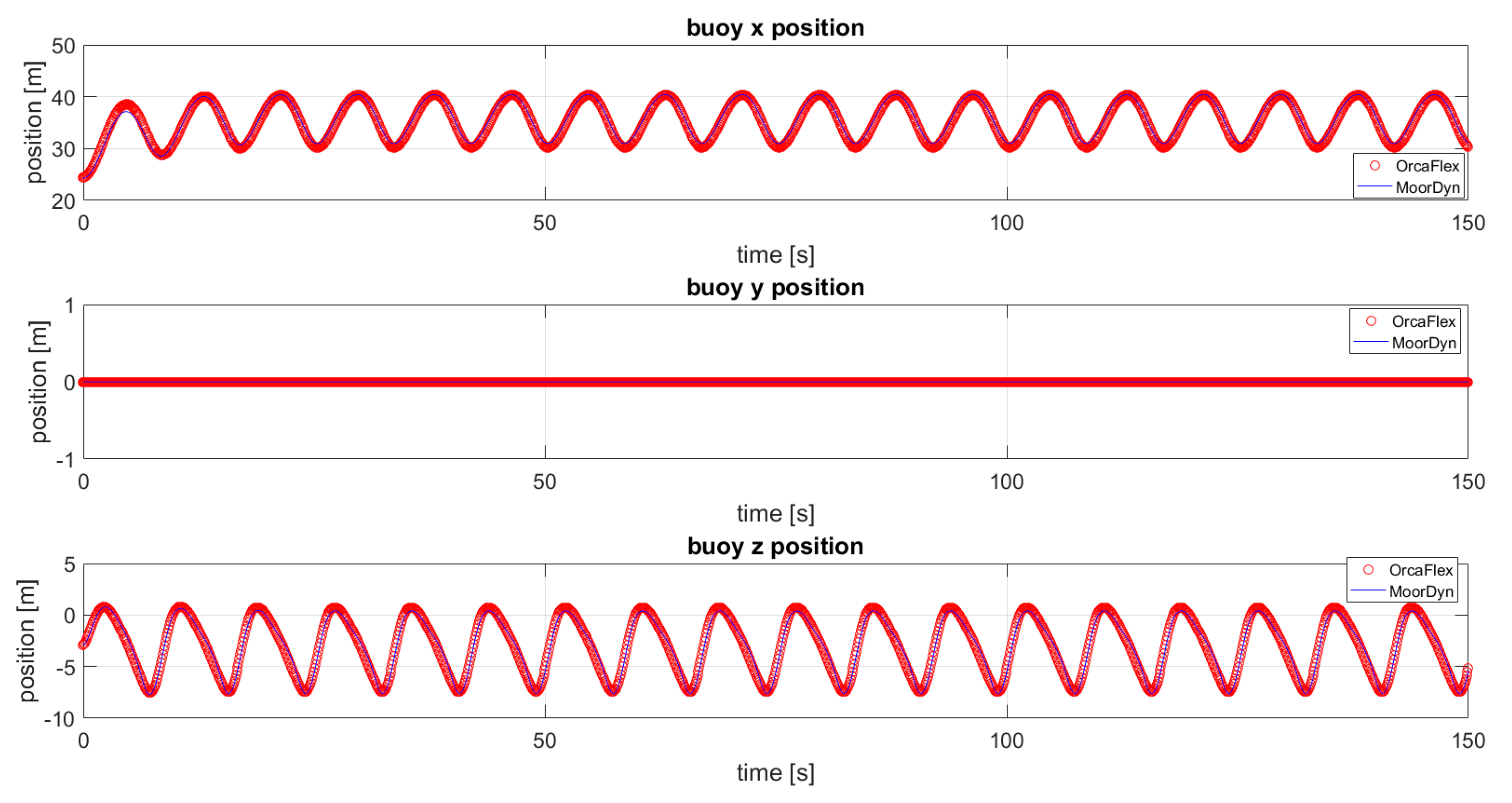
4.1. Simulation Case 1: Regular Wave
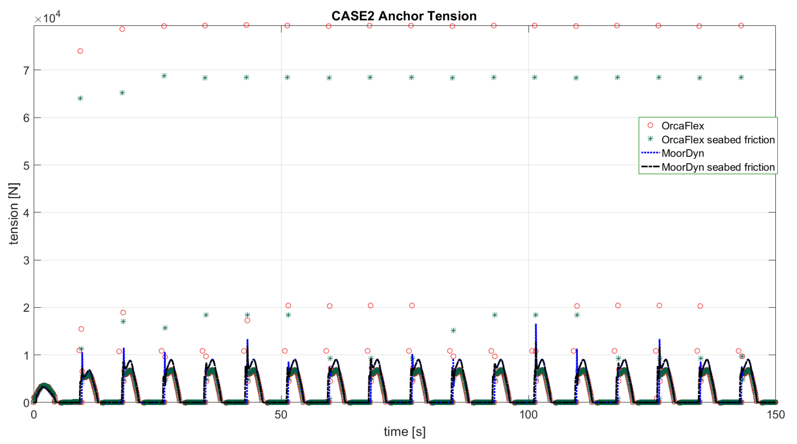
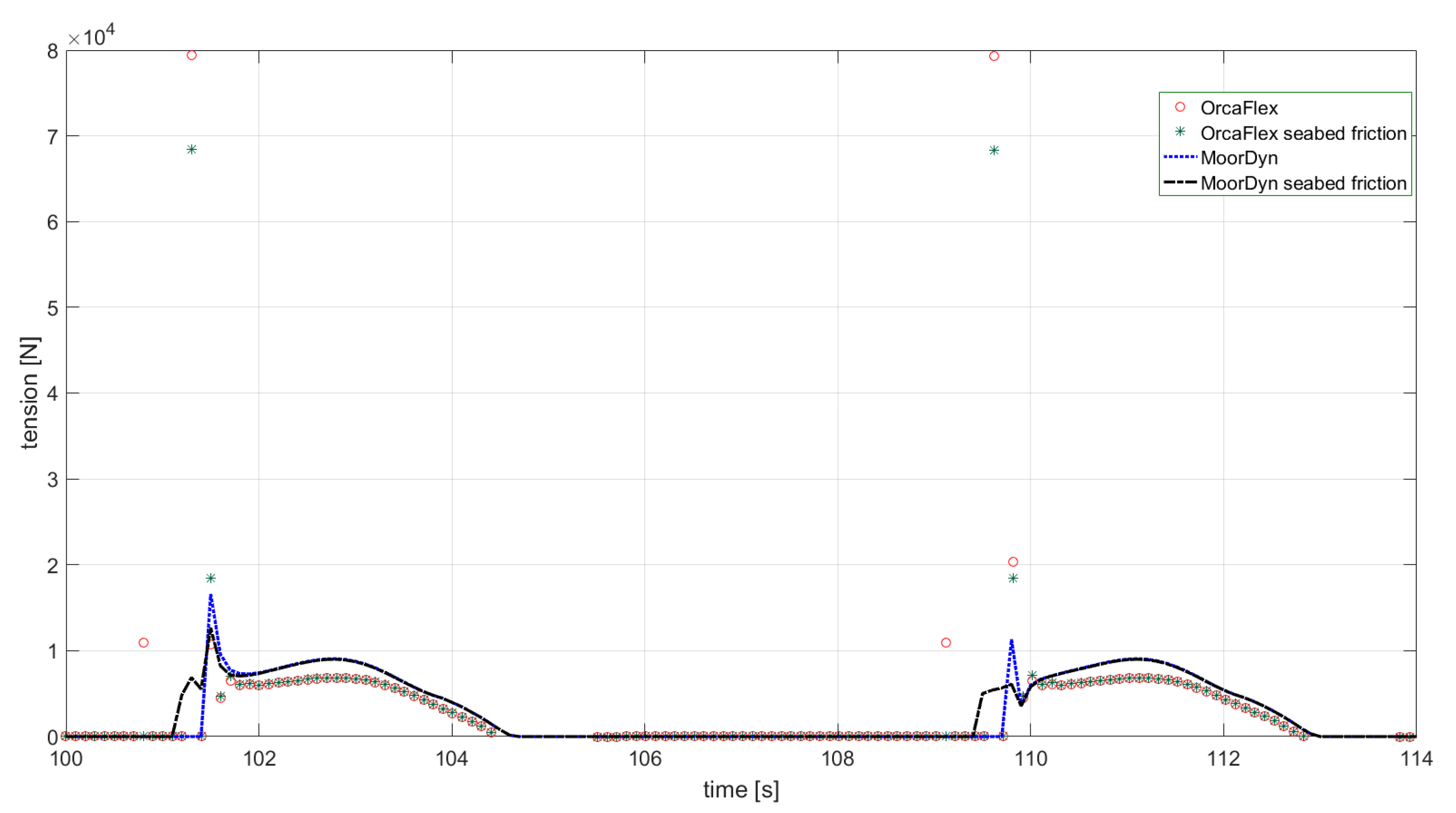
4.2. Simulation Case 2: Regular Wave and Seabed Friction
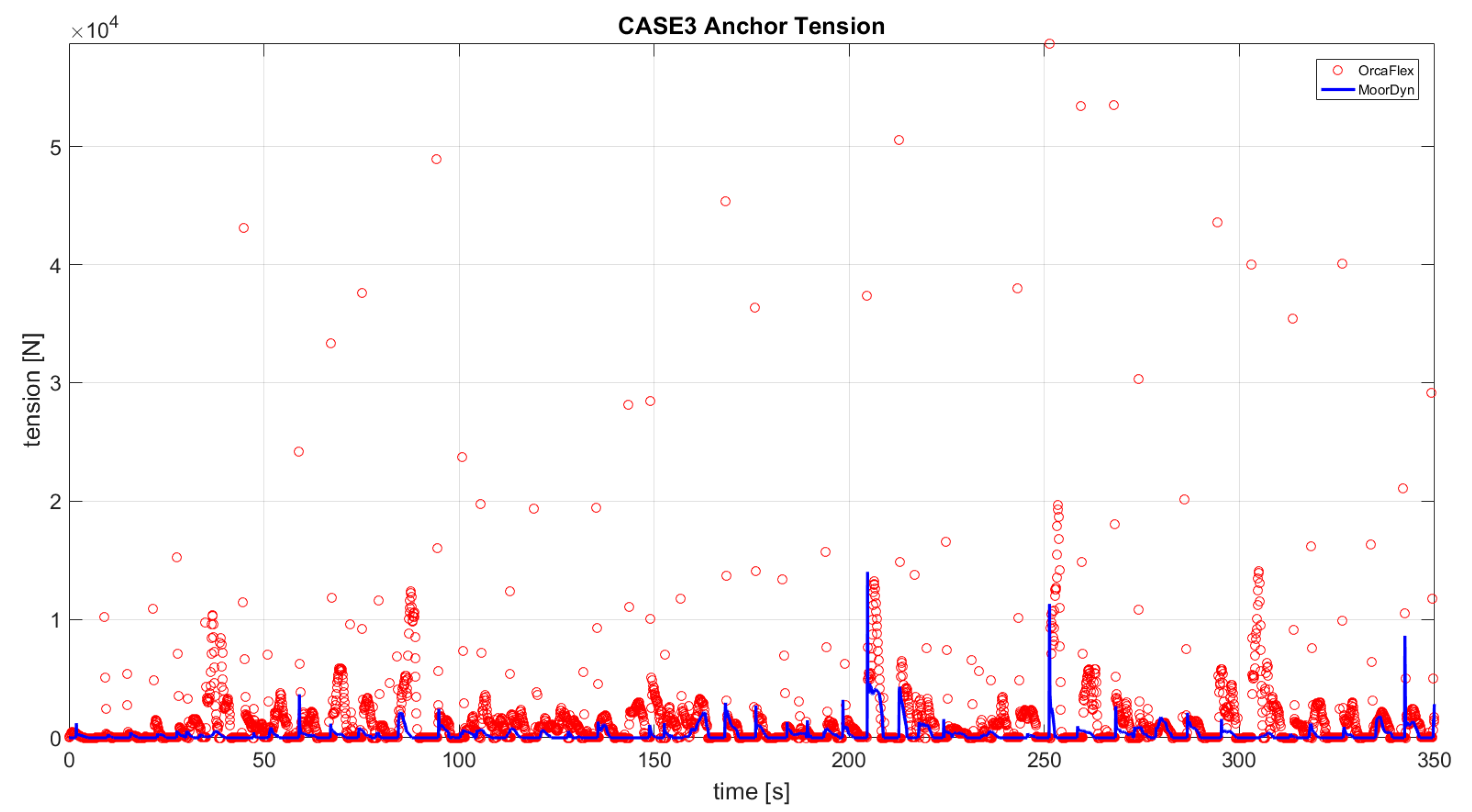
4.3. Simulation Case 3: Irregular wave
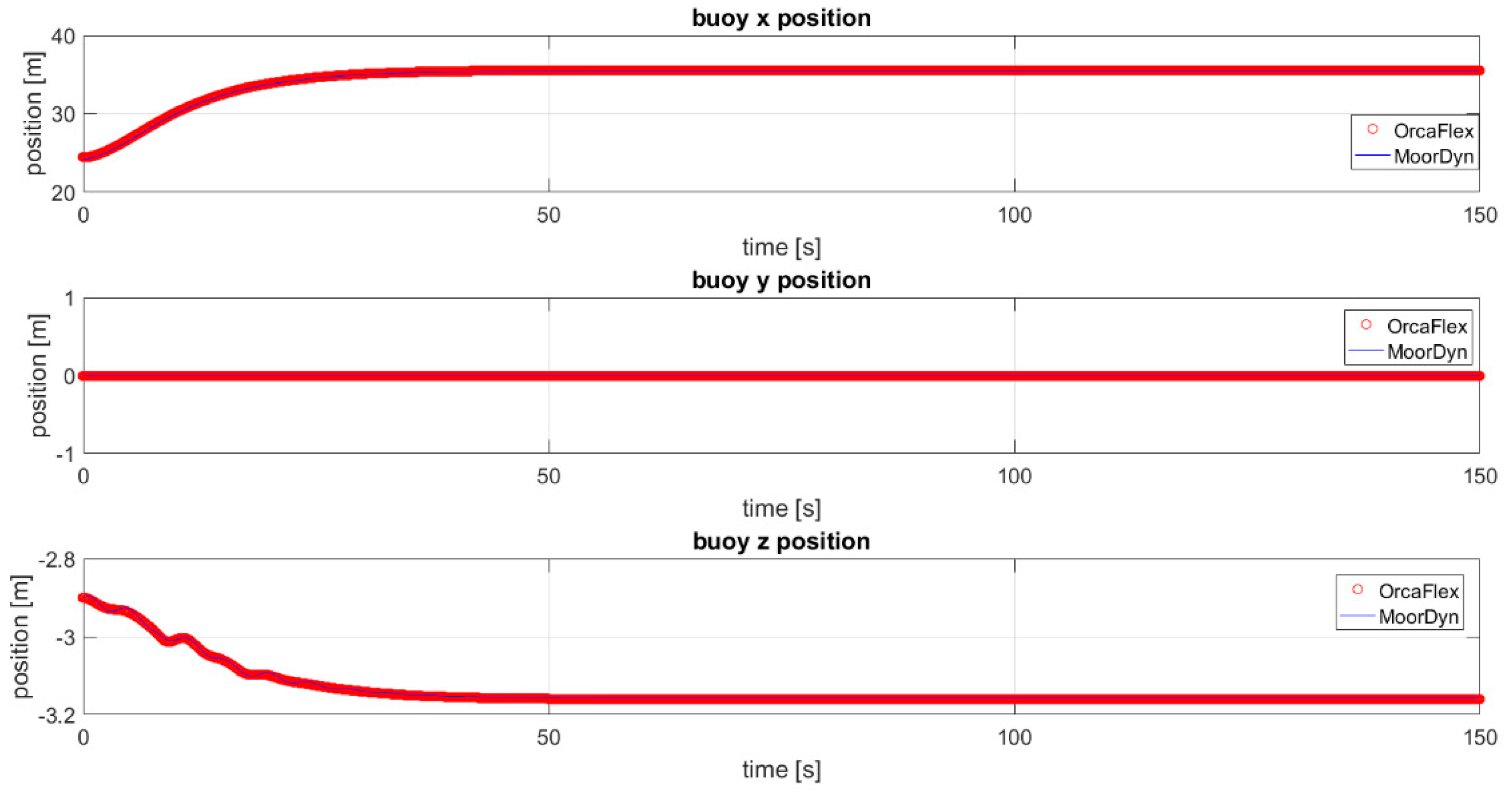
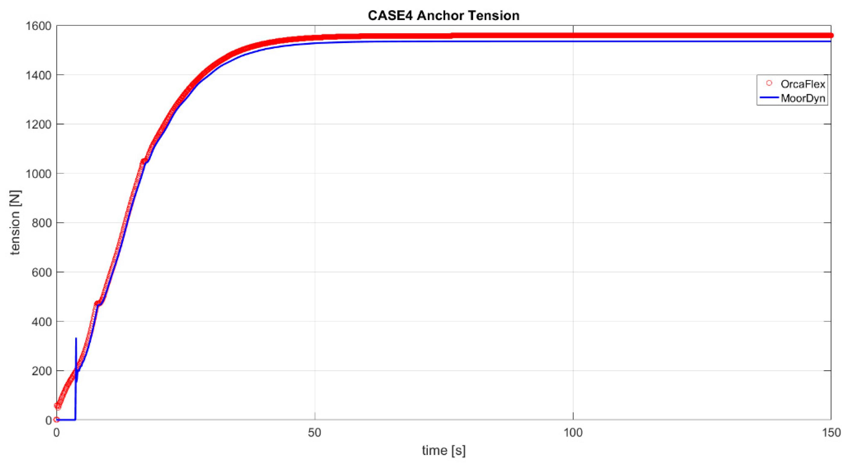
4.4. Simulation Case 4: Current
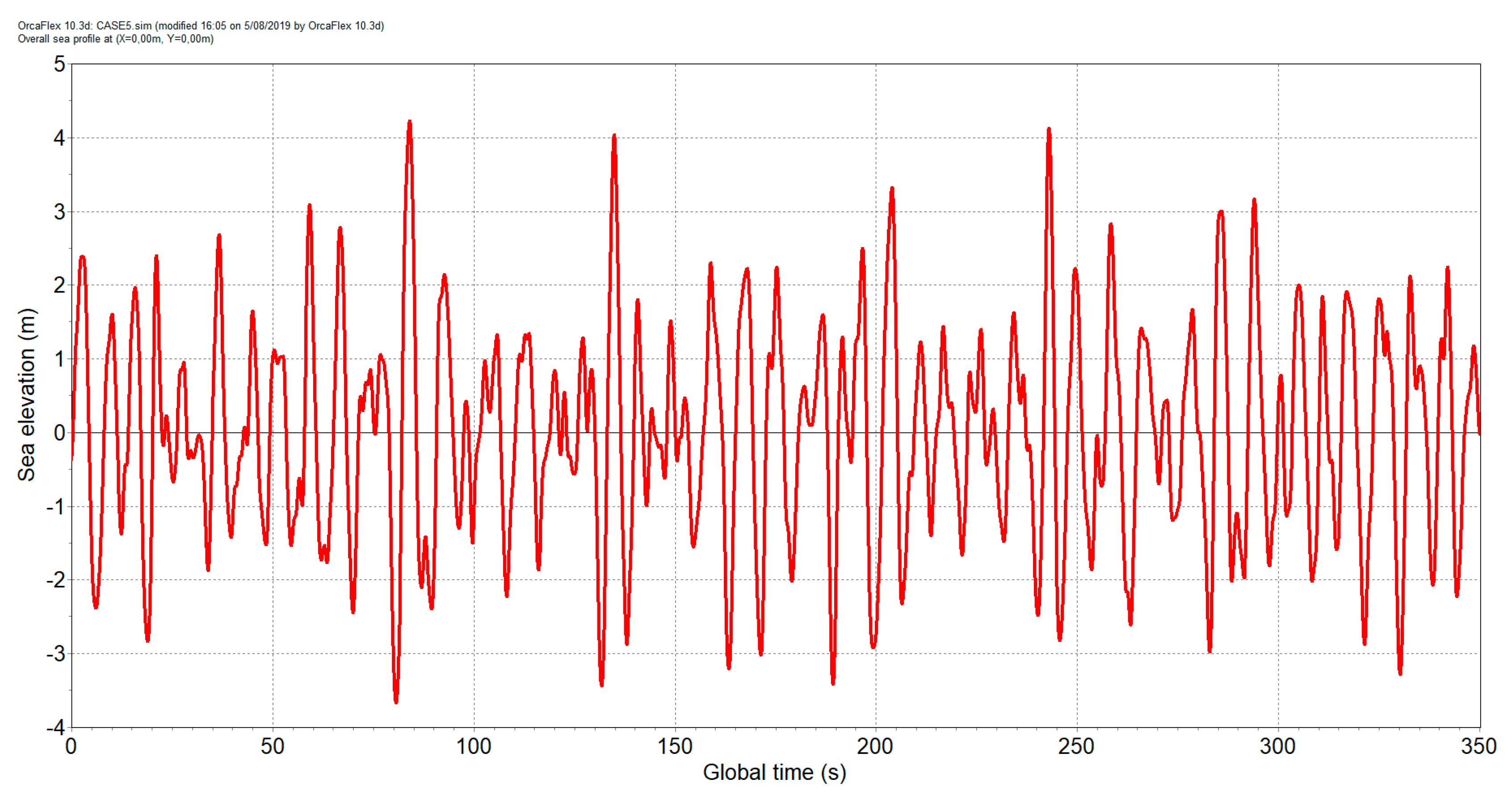
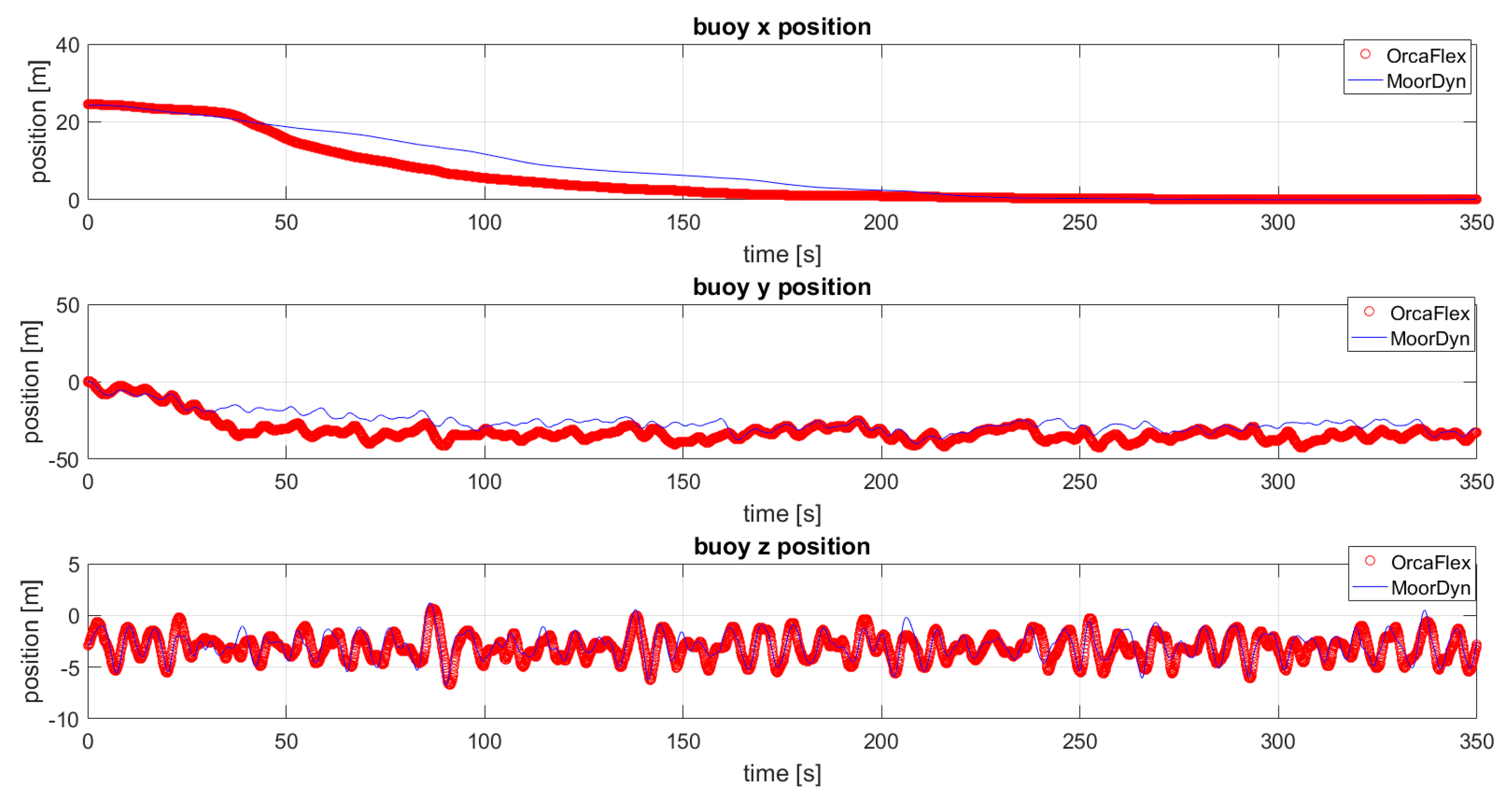
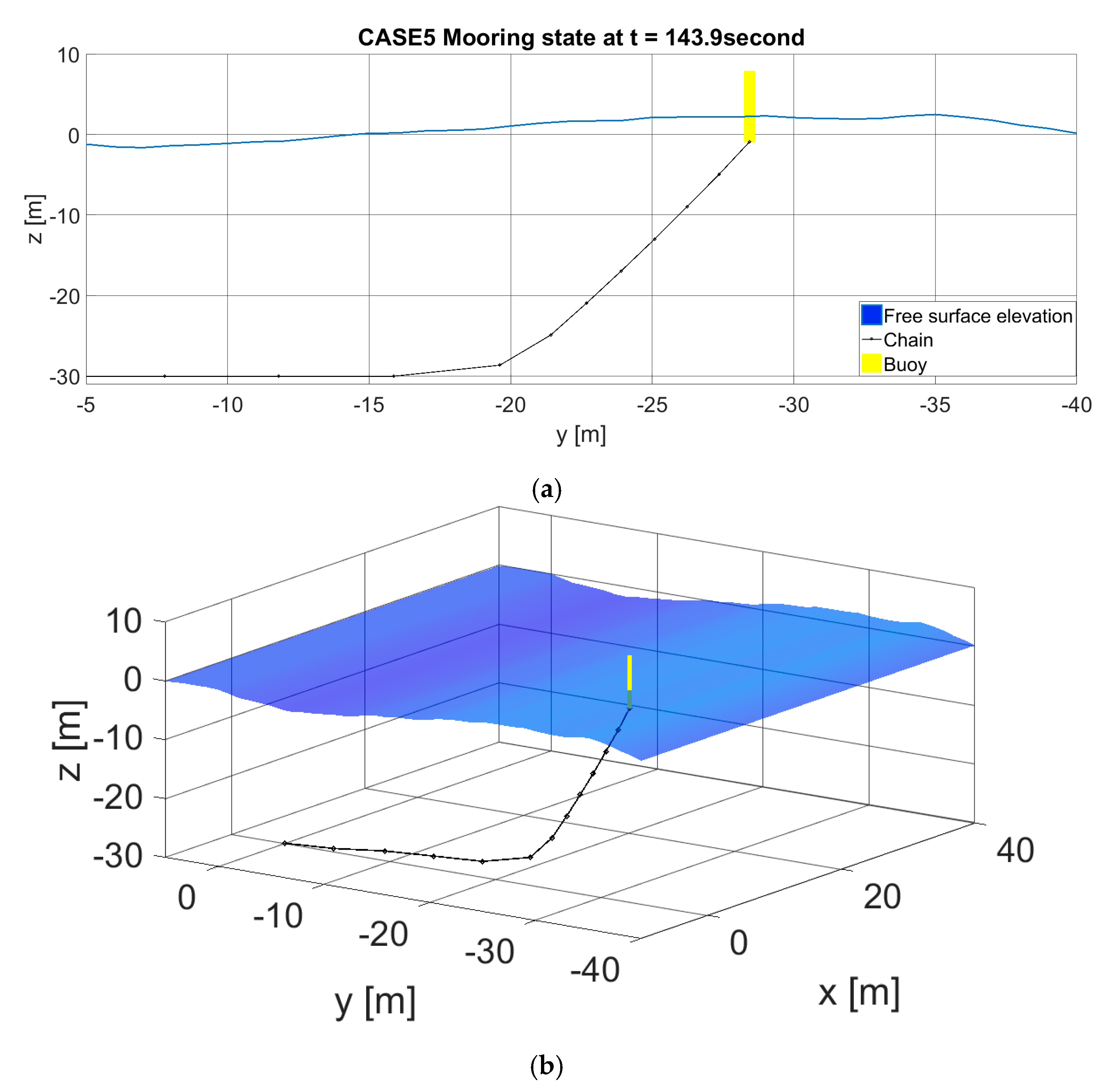
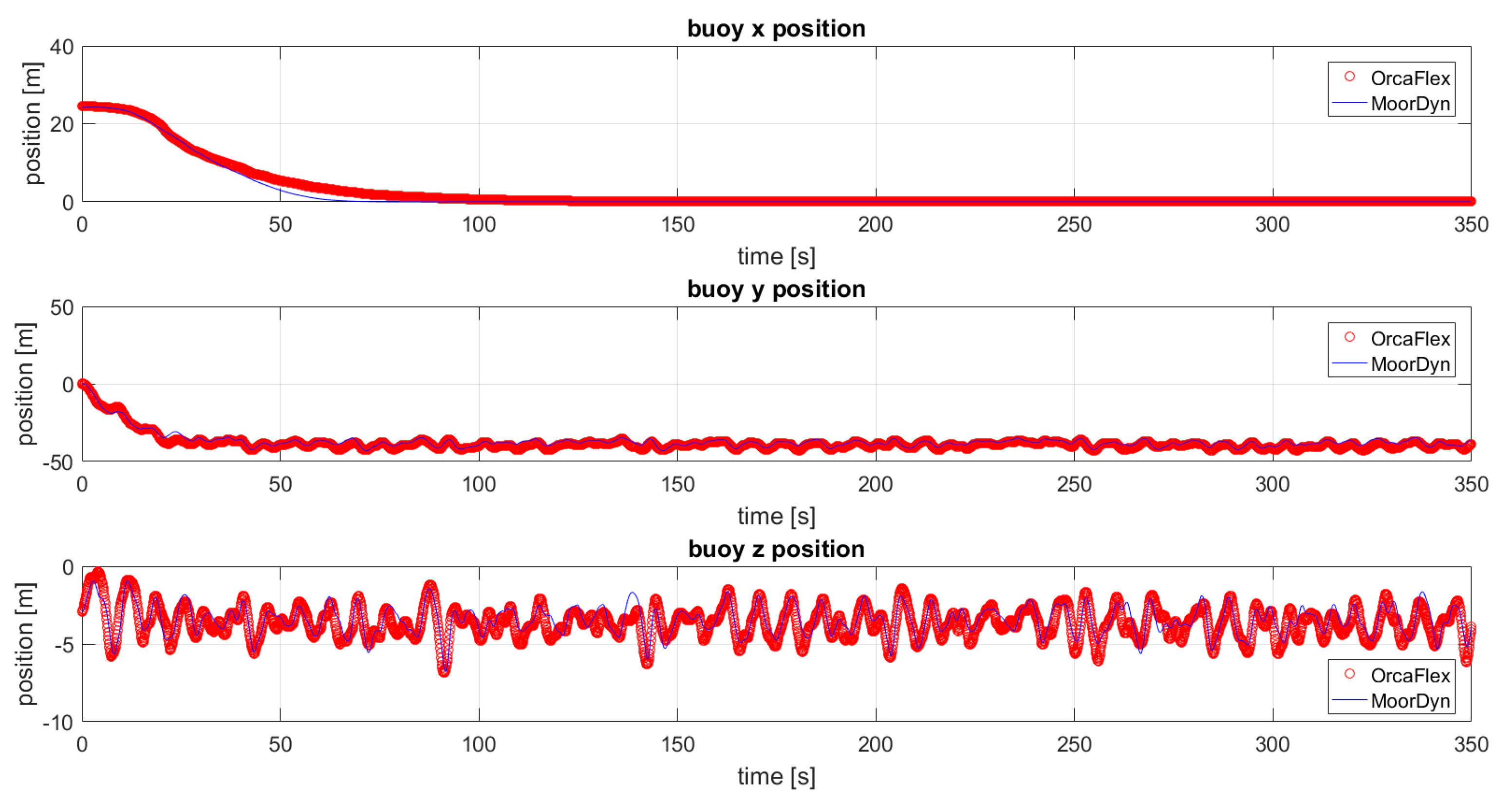
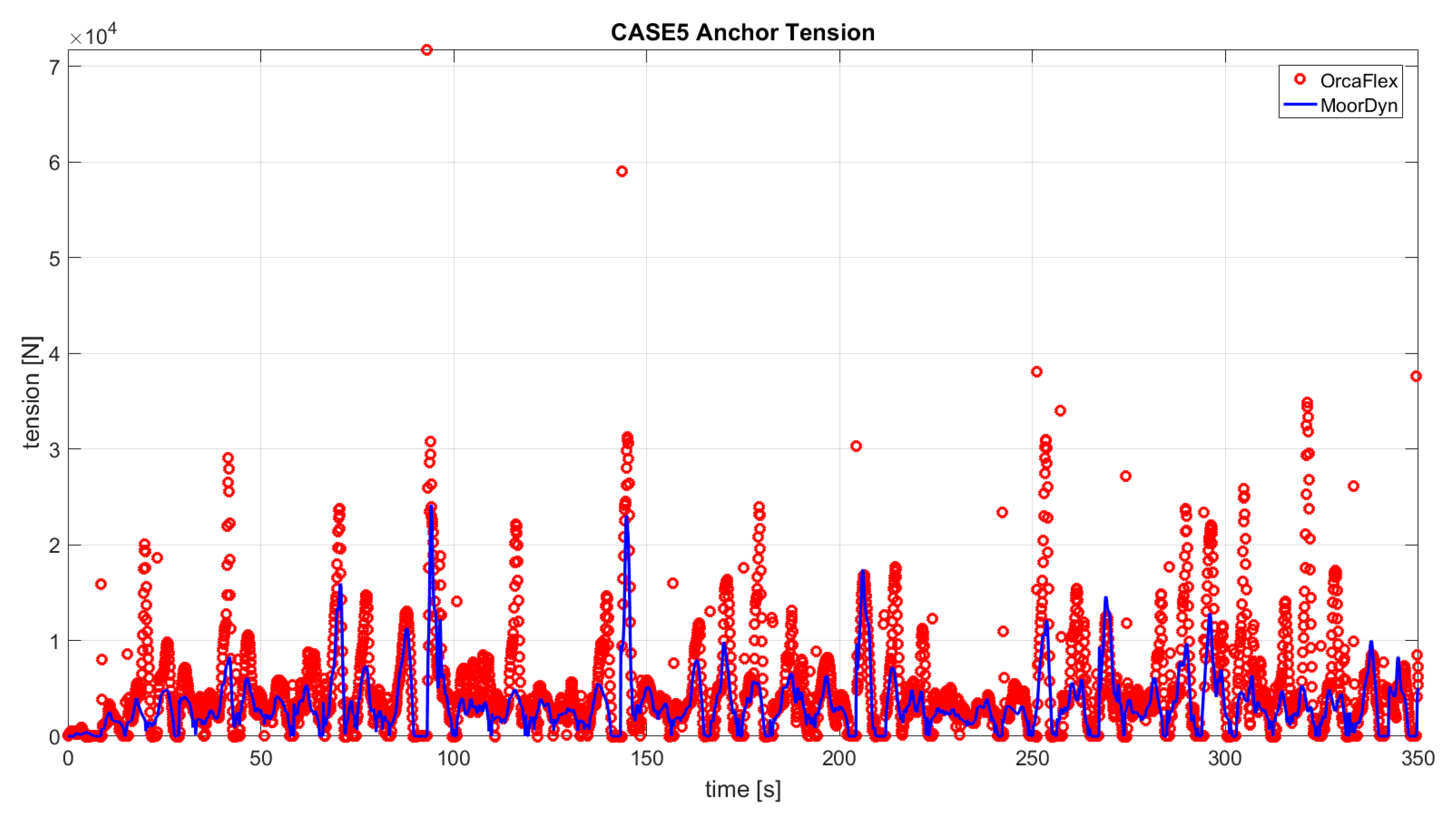
4.5. Simulation Case 5: Irregular Wave and Current
4.6. Summary of Anchor Forces
5. Conclusions and Future Work
Author Contributions
Funding
Acknowledgments
Conflicts of Interest
Appendix A. Integration Scheme
Appendix B

| Wave Components | |||
|---|---|---|---|
| Frequency | Period | Amplitude | Phase Angle |
| [Hz] | [s] | [m] | [rad] |
| 0.061 | 16.262 | 0.002 | 2.308 |
| 0.068 | 14.784 | 0.015 | 3.02 |
| 0.074 | 13.440 | 0.065 | 0.463 |
| 0.082 | 12.218 | 0.172 | 0.034 |
| 0.090 | 11.107 | 0.327 | 2.181 |
| 0.099 | 10.098 | 0.504 | 2.15 |
| 0.109 | 9.180 | 0.72 | 1.369 |
| 0.120 | 8.345 | 0.873 | 0.837 |
| 0.132 | 7.586 | 0.832 | 5.658 |
| 0.145 | 6.897 | 0.691 | 2.43 |
| 0.159 | 6.270 | 0.604 | 2.799 |
| 0.175 | 5.700 | 0.533 | 4.159 |
| 0.193 | 5.182 | 0.461 | 0.101 |
| 0.212 | 4.711 | 0.393 | 4.089 |
| 0.234 | 4.282 | 0.332 | 4.062 |
| 0.257 | 3.893 | 0.279 | 2.029 |
| 0.283 | 3.539 | 0.233 | 5.376 |
| 0.311 | 3.217 | 0.194 | 2.521 |
| 0.342 | 2.925 | 0.161 | 1.3 |
| 0.376 | 2.659 | 0.133 | 6.086 |
| 0.414 | 2.417 | 0.11 | 3.76 |
| 0.455 | 2.198 | 0.091 | 4.228 |
| 0.501 | 1.998 | 0.076 | 2.871 |
| 0.551 | 1.816 | 0.062 | 2.074 |
| 0.606 | 1.651 | 0.052 | 0.631 |
| 0.666 | 1.501 | 0.043 | 4.747 |
| 0.733 | 1.364 | 0.035 | 3.806 |
| 0.806 | 1.240 | 0.029 | 4.518 |
| 0.887 | 1.128 | 0.024 | 5.638 |
References
- Aypa, M. Mussel Culture. In Selected Papers on Mollusk Culture 1990; Fisheries and Aquaculture Department—UNDP/FAO Regional Seafarming Development and Demonstration Project (RAS/90/002)—National Inland Fisheries Institute; Kasetsart University Campus: Bangkok, Thailand, 1990. [Google Scholar]
- Morse, D.; Rice, M.A. Mussel Aquaculture in the Northeast; NRAC Publication: College Park, MD, USA, 2010; Volume 211. [Google Scholar]
- Danioux, C.; Bompais, X.; Paquotte, P.; Loste, C. Offshore Mollusc Production in the Mediterranean Basin; CIHEAM: Zaragoza, Spain, 2000; pp. 115–140. [Google Scholar]
- Buck, B.H.; Berg-Pollack, A.; Assheuer, J.; Kassen, D. Technical realization of extensive aquaculture construction in offshore wind farms: Consideration of the mechanical loads. In Proceedings of the 25th International Conference on Offshore Mechanics and Arctic Engineering, Hamburg, Germany, 4–9 June 2006. [Google Scholar]
- Stevens, C.; Plew, D.; Hartsein, N.; Fredriksson, D. The physics of open-water shellfish aquaculture. Aquac. Eng. 2008, 38. [Google Scholar] [CrossRef]
- Aquastructures. Available online: https://aquastructures.no/en/aquasim-2/ (accessed on 7 August 2019).
- Lopez, J.; Hurtado, C.F.; Gomez, A.; Zamora, V. Stress analysis of a submersible longline culture system through dynamic simulation. Latin Am. J. Aquat. Res. 2017, 45. [Google Scholar] [CrossRef]
- Lien, E.; Fredheim, A. Development of Longtube Mussel Systems for Cultivation of Mussels. In Proceedings of the OOA IV: Open Ocean Aquaculture IV Symposium, St. Andrews, NB, Canada, 17–20 June 2001. [Google Scholar]
- Ormberg, H. Non-Linear Response Analysis of Floating Fish Farm Systems. Ph.D. Thesis, Division of Marine Structures, Norwegian Institute of Technology, University of Trondheim, Trondheim, Norway, 1991. [Google Scholar]
- Raman-Nair, W.; Colbourne, B.; Gagnon, M.; Bergeron, P. Numerical model of a mussel longline system: Coupled dynamics. Ocean Eng. 2008, 35. [Google Scholar] [CrossRef]
- Walton, T.S.; Polachek, H. Calculation of Nonlinear Transient Motion of Cables; Technical Report; David Taylor Model Basin: Washington, DC, USA, 1959. [Google Scholar]
- Huang, S. Dynamic Analysis of Three-Dimension Marine Cables. Ocean Eng. 1994, 21, 587–605. [Google Scholar] [CrossRef]
- Khan, N.U.; Ansari, K.A. On the Dynamics of a Multicomponent Mooring Line. Comput. Struct. 1986, 22, 311–334. [Google Scholar] [CrossRef]
- Palm, J.; Moura, P.G.; Eskilsson, C.; Taveira, P.F.; Bergdahl, L. Simulation of mooring cable dynamics using a discontinuous galerkin method. In Proceedings of the V International Conference on Computational Methods in Marine Engineering, Hamburg, Germany, 29–31 May 2013. [Google Scholar]
- Hall, M.; Goupee, A. Validation of a lumped-mass mooring line model with DeepCwind semisubmersible model test data. Ocean Eng. 2015, 104, 590–603. [Google Scholar] [CrossRef] [Green Version]
- Hall, M. MoorDyn User’s Guide; Tech. Rep.; University of Prince Edward Island: Charlottetown, PEI, Canada, 2017. [Google Scholar]
- Garret, D.L. Dynamic Analysis of Slender Rods. J. Energy Resour. Technol. 1982, 104, 302–306. [Google Scholar] [CrossRef]
- Malahy, R.C. A Nonlinear Finite Element Method for the Analysis of the Offshore Pipelaying Problem. Ph.D. Thesis, Rice University, Houston, TX, USA, 1985. [Google Scholar]
- McNamara, J.F.; O’Brien, P.J.; Gilroy, S.G. Nonlinear analysis of flexible risers using hybrid finite elements. J. Offshore Mech. Arct. Eng. 1988, 110, 197–204. [Google Scholar] [CrossRef]
- Hall, M.; Buckham, B.; Crawford, C. Evaluating the importance of mooring line model fidelity in floating offshore wind turbine simulations. Wind Energy 2014, 17, 1835–1853. [Google Scholar] [CrossRef]
- Buck, B.H. Experimental trials on the feasibility of offshore seed production of the mussel Mytilus edulis in the German Bight: Installation, technical requirements and environmental conditions. Helgol. Mar. Res. 2007, 61. [Google Scholar] [CrossRef]
- Gagnon, M.; Bergeron, P. Observations of the loading and motion of a submerged mussel longline at an open ocean site. Aquac. Eng. 2017, 78. [Google Scholar] [CrossRef]
- Orcina.com. Available online: https://www.orcina.com/ (accessed on 7 January 2019).
- Orcina. OrcaFlex Manual Version 9.1a; Tech. Rep.; Orcina Ltd.: Ulverston, UK, 2010. [Google Scholar]
- Andersen, M.T.; Wendt, F.F.; Robertson, A.N.; Jonkman, J.M.; Hall, M. Verification and Validation of Multisegmented Mooring Capabilities in FAST v8. In Proceedings of the ISOPE2016: International Ocean and Polar Engineering Conference, Rhodes, Greece, 26 June–2 July 2016. [Google Scholar]
- Press, W.H.; Teukolsky, S.A.; Vetterling, W.T.; Flannery, B.P. Numerical Recipes: The Art of Scientific Computing, 3rd ed.; Cambridge University Press: Cambridge, UK, 2007. [Google Scholar]
- Airy, G.B. Tides and waves. In Encyclopaedia Metropolitana; Various Publishers: London, UK, 1841; Volume V, pp. 241–396. [Google Scholar]
- Holthuijsen, L.H. Waves in Oceanic and Coastal Waters; Cambridge University Press: Cambridge, UK, 2007. [Google Scholar]
- Wheeler, J.D. Method for calculating forces produced by irregular waves. J. Pet. Technol. 1970, 22. [Google Scholar] [CrossRef]
- Fenton, J.D. The Numerical Solution of Steady Water Wave Problems. Comput. Geosci. 1988, 14, 357–368. [Google Scholar] [CrossRef]
- Svendsen, I.A. Introduction to Nearshore Hydrodynamics; World Scientific Publishing Co. Pte Ltd.: Singapore, 2005. [Google Scholar]
- Kirby, J.T.; Chen, T.M. Surface waves on vertically sheared flows. J. Geophys. Res. Oceans 1989, 94, 1013–1027. [Google Scholar] [CrossRef]
- Rusu, L.; Soares, C.G. Modelling the wave–current interactions in an offshore basin using the SWAN model. Ocean. Eng. 2011, 38, 63–76. [Google Scholar] [CrossRef]
- Huang, N.E.; Chen, D.T.; Tung, C.C.; Smith, J.R. Interactions between Steady Non-Uniform Currents and Gravity Waves with Applications for Current Measurements. J. Phys. Oceanogr. 1972, 2, 420–431. [Google Scholar] [CrossRef]
- Belibassakis, K.; Touboul, J. A Nonlinear Coupled-Mode Model for Waves Propagating in Vertically Sheared Currents in Variable Bathymetry-CollinearWaves and Currents. Fluids 2019, 4, 61. [Google Scholar] [CrossRef]
- Pascolo, S.; Petti, M.; Bosa, S. Wave–Current Interaction: A 2DH Model for Turbulent Jet and Bottom-Friction Dissipation. Water 2018, 10, 392. [Google Scholar] [CrossRef]
- Melito, L.; Postacchini, M.; Darvini, G.; Brocchini, M. Waves and Currents at a River Mouth: The Role of Macrovortices, Sub-Grid Turbulence and Seabed Friction. Water 2018, 10, 550. [Google Scholar] [CrossRef]
- Morison, J.R.; O’Brien, M.P.; Johnson, J.W.; Schaaf, S.A. The force exerted by surface waves on piles. J. Pet. Technol. 1950, 2. [Google Scholar] [CrossRef]
- Bureau Veritas. BV-NR-493: Classification of Mooring Systems for Permanent and Mobile Offshore Units; Bureau Veritas: Neuilly sur Seine Cedex, France, 2015. [Google Scholar]
- Det Norske Veritas Germanischer Lyold As. DNVGL-OS-E301: Position Mooring; DNVGL: Hovik, Norway, 2015. [Google Scholar]
- Hall, M. Efficient modelling of seabed friction and multi-floater mooring systems in MoorDyn. In Proceedings of the 12th European Wave and Tidal Energy Conference, Cork, Ireland, 27 August–1 September 2017. [Google Scholar]


| Line Type [-] | Dry Mass per Length [kg/m] | Nominal Diameter [m] | Line Length [m] |
|---|---|---|---|
| Chain (Grade 3 steel) | 10.910 | 0.022 | 108 |
| Backbone (Movline Plus 8 strands) | 2.1 | 0.068 | 57 |
| Mussel sock (fully grown mussels) | 21.8 | 0.15 | 145 |
| Buoy Type [-] | Outer Diameter [m] | Dry Mass [kg] | Length [m] | Volume [m3] | Quantity [-] |
|---|---|---|---|---|---|
| SPAR buoy | 0.790 | 2500 | 8.865 | 4.345 | 2 |
| Anchor Type [-] | Dry Mass [kg] | Quantity [-] |
|---|---|---|
| Gravity | 15000 | 2 |
| Danforth | 2500 | 2 |
| Equivalent Diameter [m] | Dry Mass per Length [kg/m] | Axial Stiffness [N] | Chain Length [m] | Can [-] | Cat [-] | Cdn [-] | Cdt [-] |
|---|---|---|---|---|---|---|---|
| 0.042 | 10.910 | 48884000 | 50 | 1.0 | 0.50 | 1.4 | 0.2 |
| Equivalent Diameter [m] | Dry Mass [kg] | Height [m] | Volume [m3] | Can [-] | Cat [-] | Cdn [-] | Cdt [-] |
|---|---|---|---|---|---|---|---|
| 0.790 | 1200 | 8.865 | 4.345 | 0.94 | 0.50 | 0.81 | 0.40 |
| Object Type | X [m] | Y [m] | Z [m] |
|---|---|---|---|
| Anchor | 0.00 | 0.00 | −30.00 |
| Buoy | 30.00 | 0.00 | −4.43 |
| Simulation Case | OrcaFlex min | OrcaFlex mean | OrcaFlex max | Adapted MoorDyn min | Adapted MoorDyn mean | Adapted MoorDyn max |
|---|---|---|---|---|---|---|
| 1 | 0 N | 2986 N | 79,442 N | 0 N | 2355 N | 16,597 N |
| 2 | 0 N | 2696 N | 68,756 N | 0 N | 2609 N | 12,672 N |
| 3 | 0 N | 1605 N | 58,753 N | 0 N | 293 N | 14,024 N |
| 4 | 0 N | 1406 N | 1558 N | 0 N | 1380 N | 1535 N |
| 5 | 0 N | 5058 N | 71,766 N | 0 N | 3319 N | 24,173 N |
© 2019 by the authors. Licensee MDPI, Basel, Switzerland. This article is an open access article distributed under the terms and conditions of the Creative Commons Attribution (CC BY) license (http://creativecommons.org/licenses/by/4.0/).
Share and Cite
Pribadi, A.B.K.; Donatini, L.; Lataire, E. Numerical Modelling of a Mussel Line System by Means of Lumped-Mass Approach. J. Mar. Sci. Eng. 2019, 7, 309. https://doi.org/10.3390/jmse7090309
Pribadi ABK, Donatini L, Lataire E. Numerical Modelling of a Mussel Line System by Means of Lumped-Mass Approach. Journal of Marine Science and Engineering. 2019; 7(9):309. https://doi.org/10.3390/jmse7090309
Chicago/Turabian StylePribadi, Ajie Brama Krishna, Luca Donatini, and Evert Lataire. 2019. "Numerical Modelling of a Mussel Line System by Means of Lumped-Mass Approach" Journal of Marine Science and Engineering 7, no. 9: 309. https://doi.org/10.3390/jmse7090309