Accumulation of Pore Pressure in a Soft Clay Seabed around a Suction Anchor Subjected to Cyclic Loads

Abstract
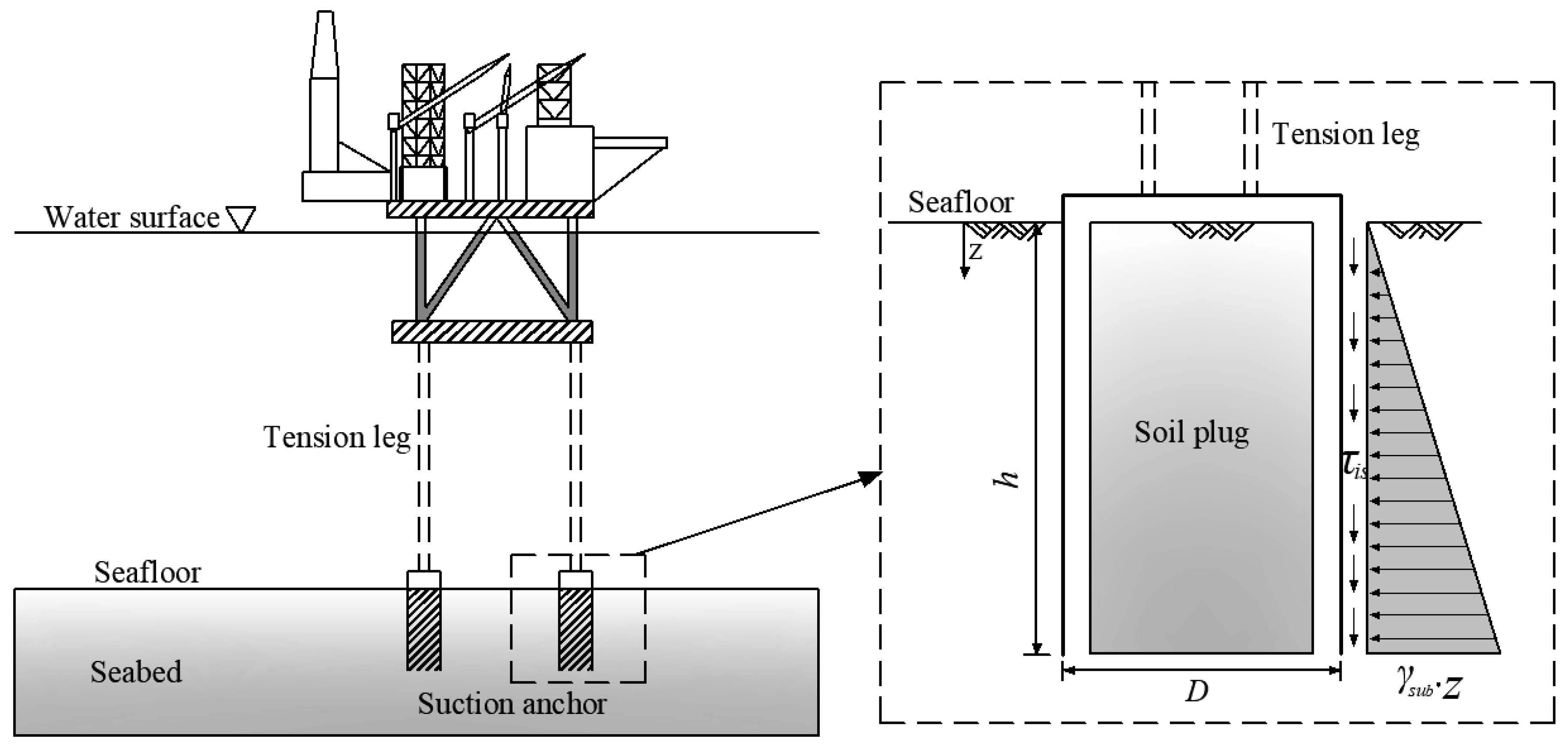
:1. Introduction
2. Theoretical Formulations and Numerical Approach
2.1. Constitutive Model
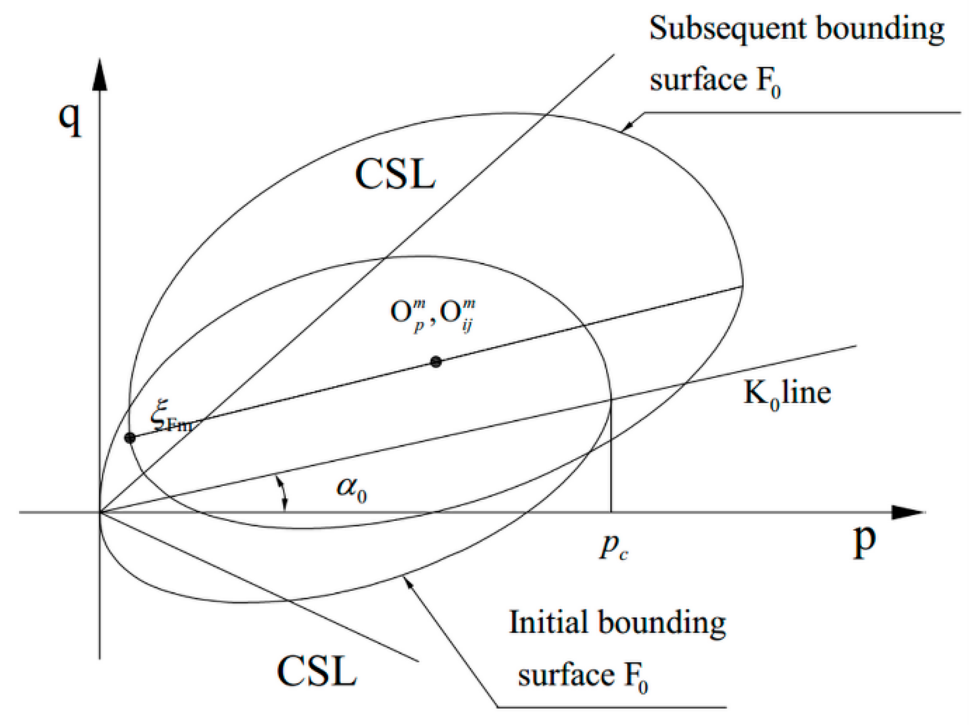
2.1.1. Anisotropic Bounding Surface
2.1.2. The Evolution of the Boundary Surface
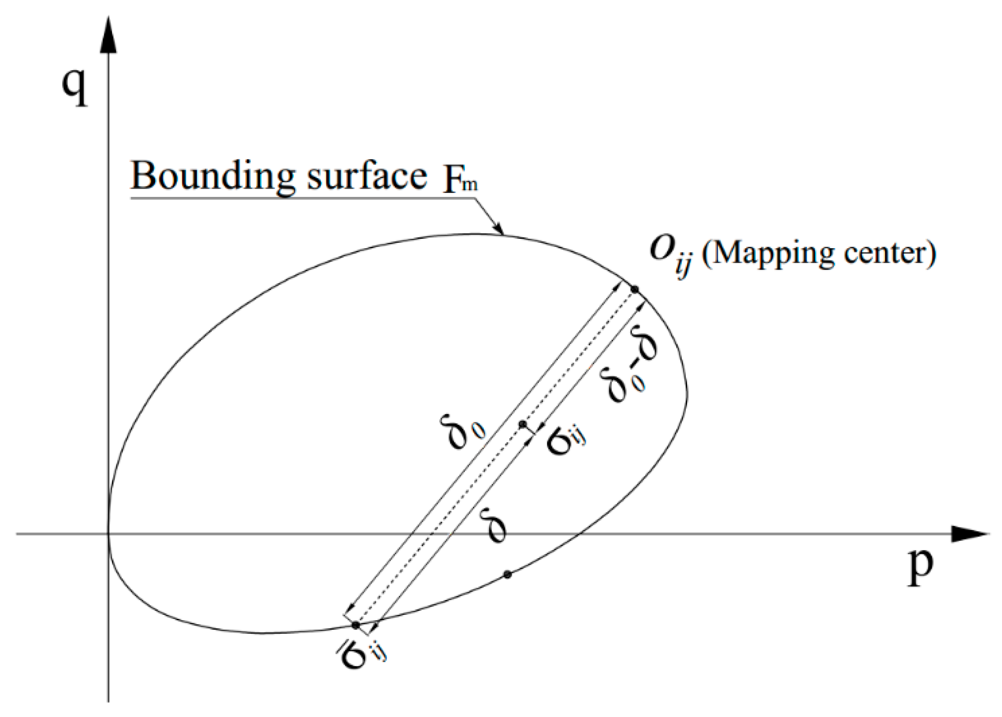
2.1.3. Mapping and Flow Rules
2.1.4. Incremental Equations
2.1.5. Hardening Modulus
2.1.6. Implicit Integration Algorithm
- 1)
- Assume that strain increment is complete elastic increment at incremental steps of n+1. For initial iteration count k = 0, these variables are defined as follows:
- 2)
- Non-linear elastic predictor:
- 3)
- Distinguish the unloading process from the loading event, according to Equation (4). (a) reloading, homological center remains constant. (b) unloading, update the homological center and the bounding surface, according to Equations (5)–(6). Then evaluate the following residuals:where l is the number of nonlinear equations. Variable A can be presented as:If the tolerance (taken as ), THEN EXITElse GO TO step 4
- 4)
- Solve the linear equations:where .
- 5)
- Update stresses and internal variable , and GO TO step (3).
- 6)
- Satisfy the convergence condition, END.
2.2. Numerical Scheme
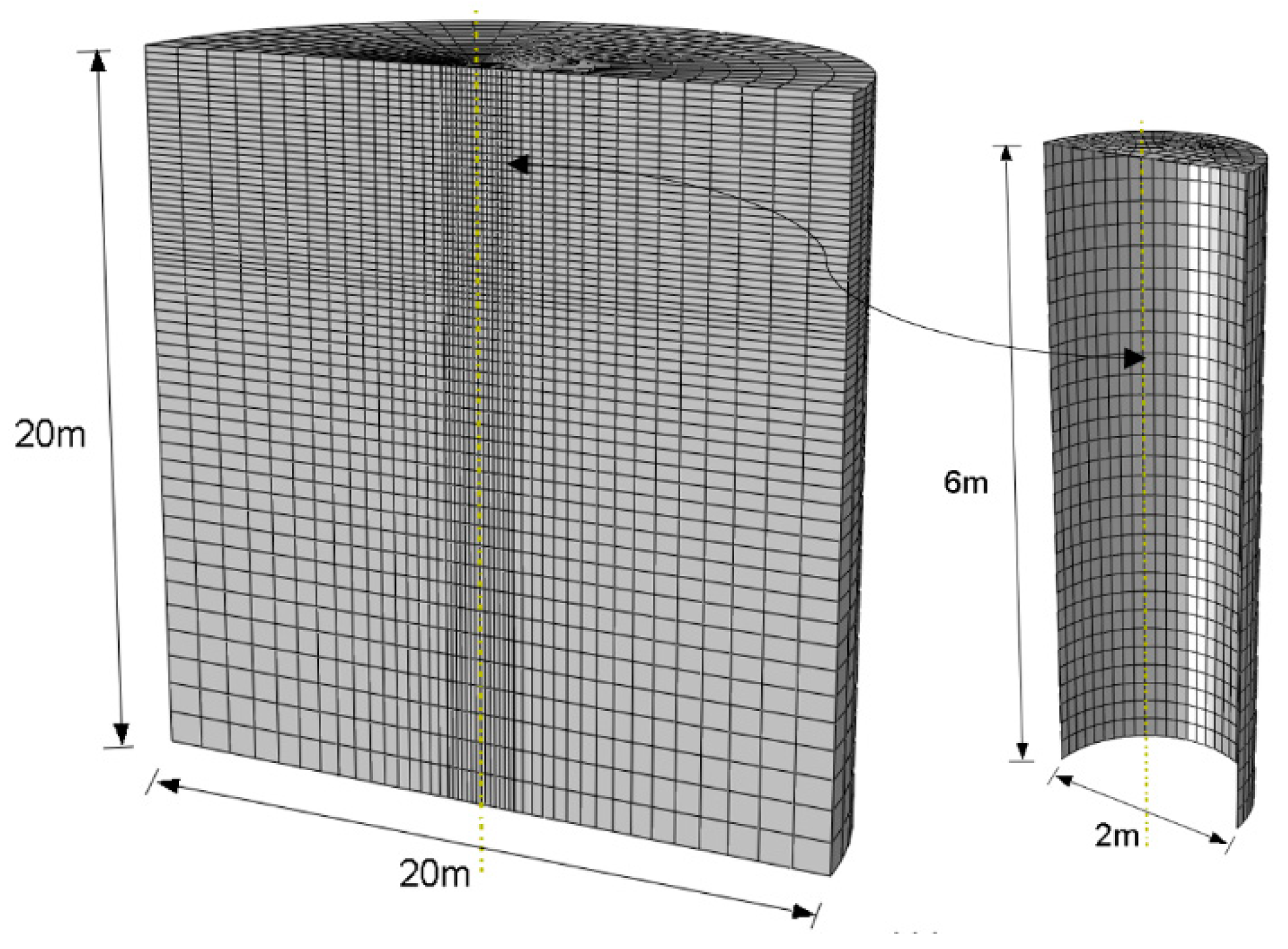
2.3. Meshing and Boundary Conditions
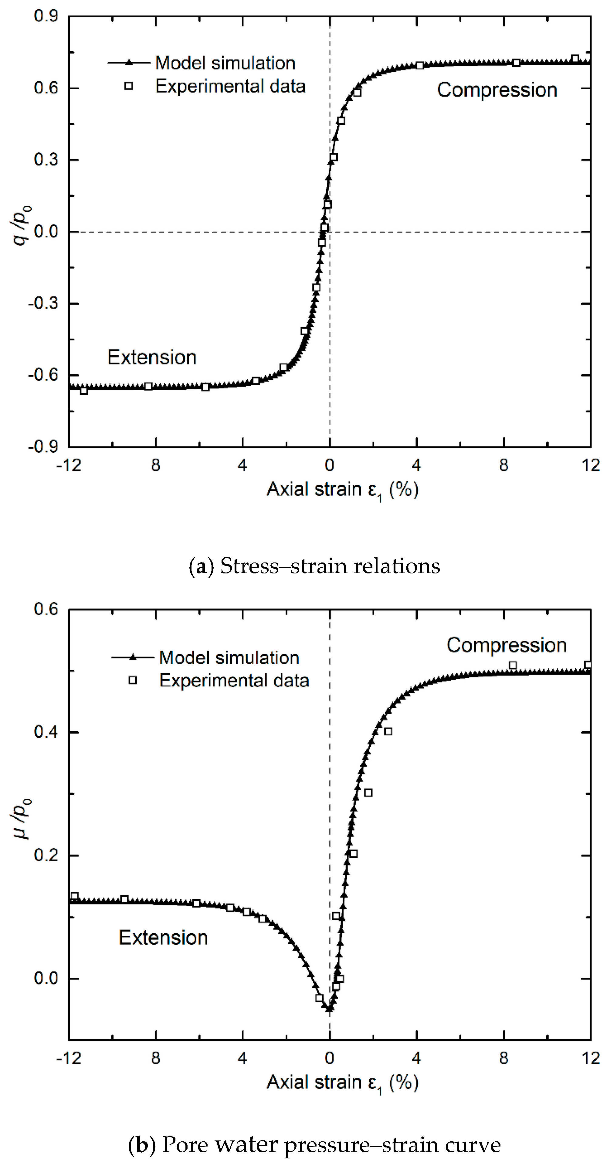
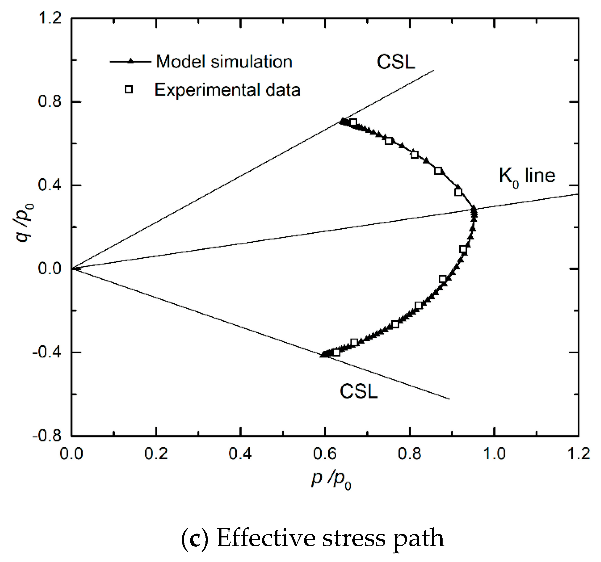
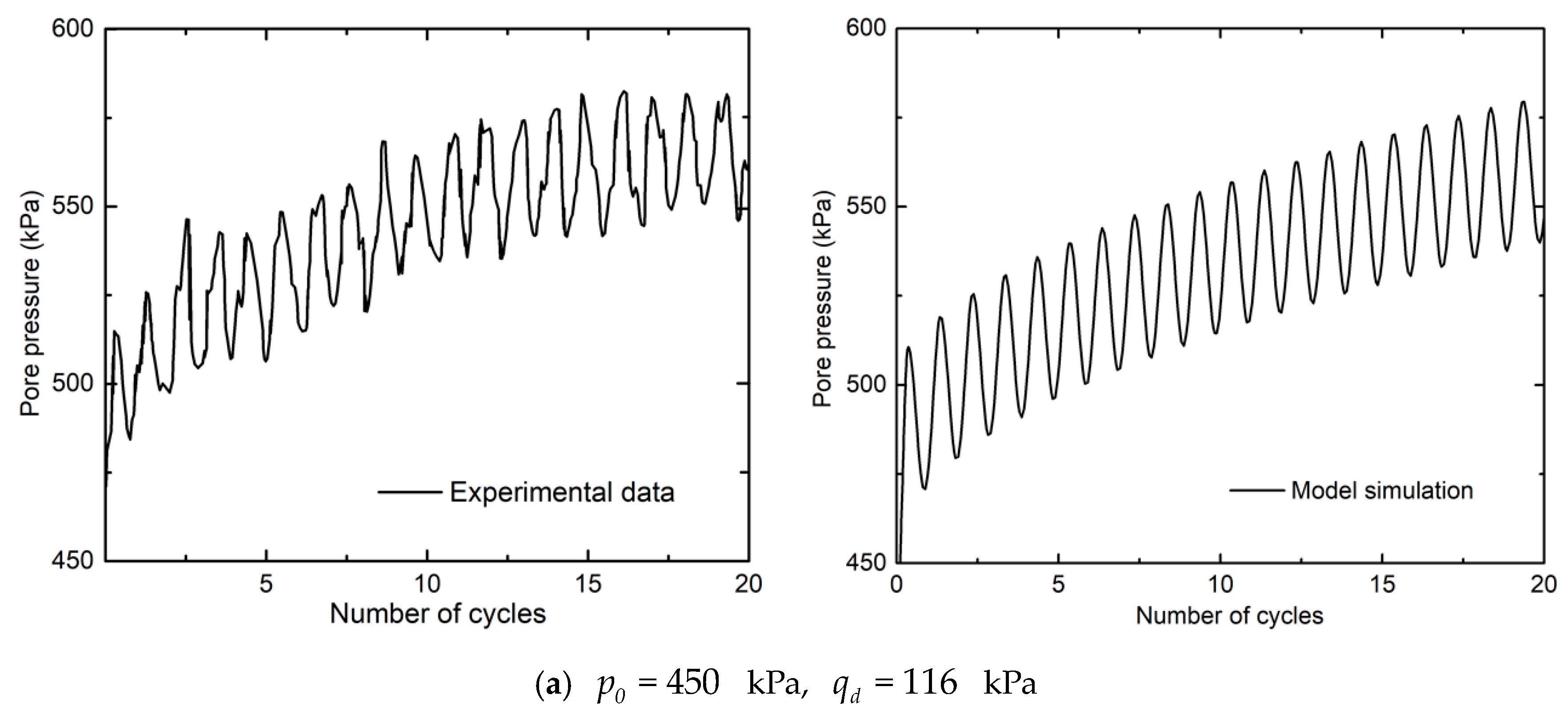
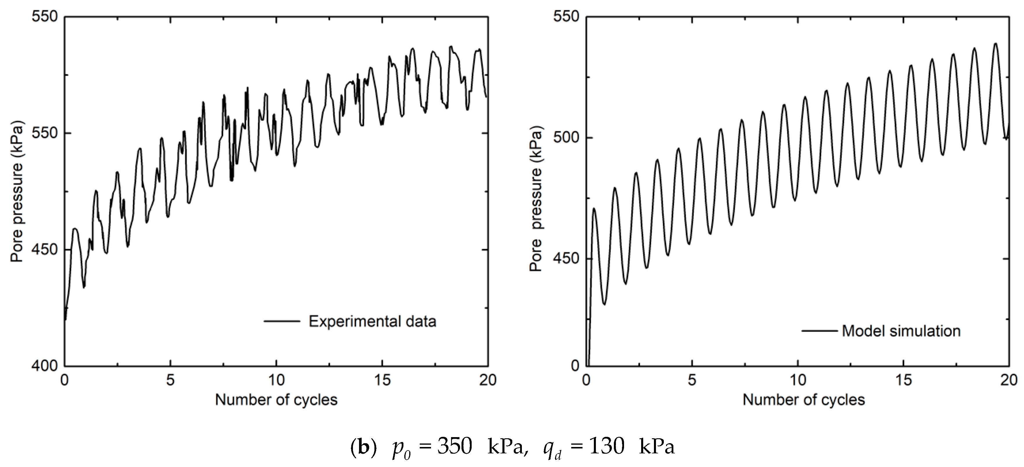
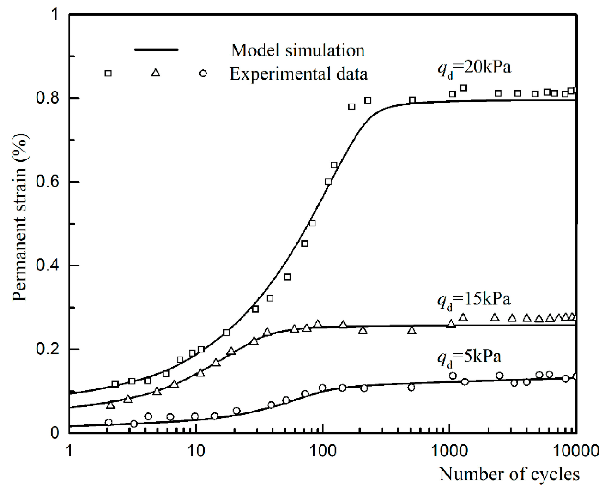
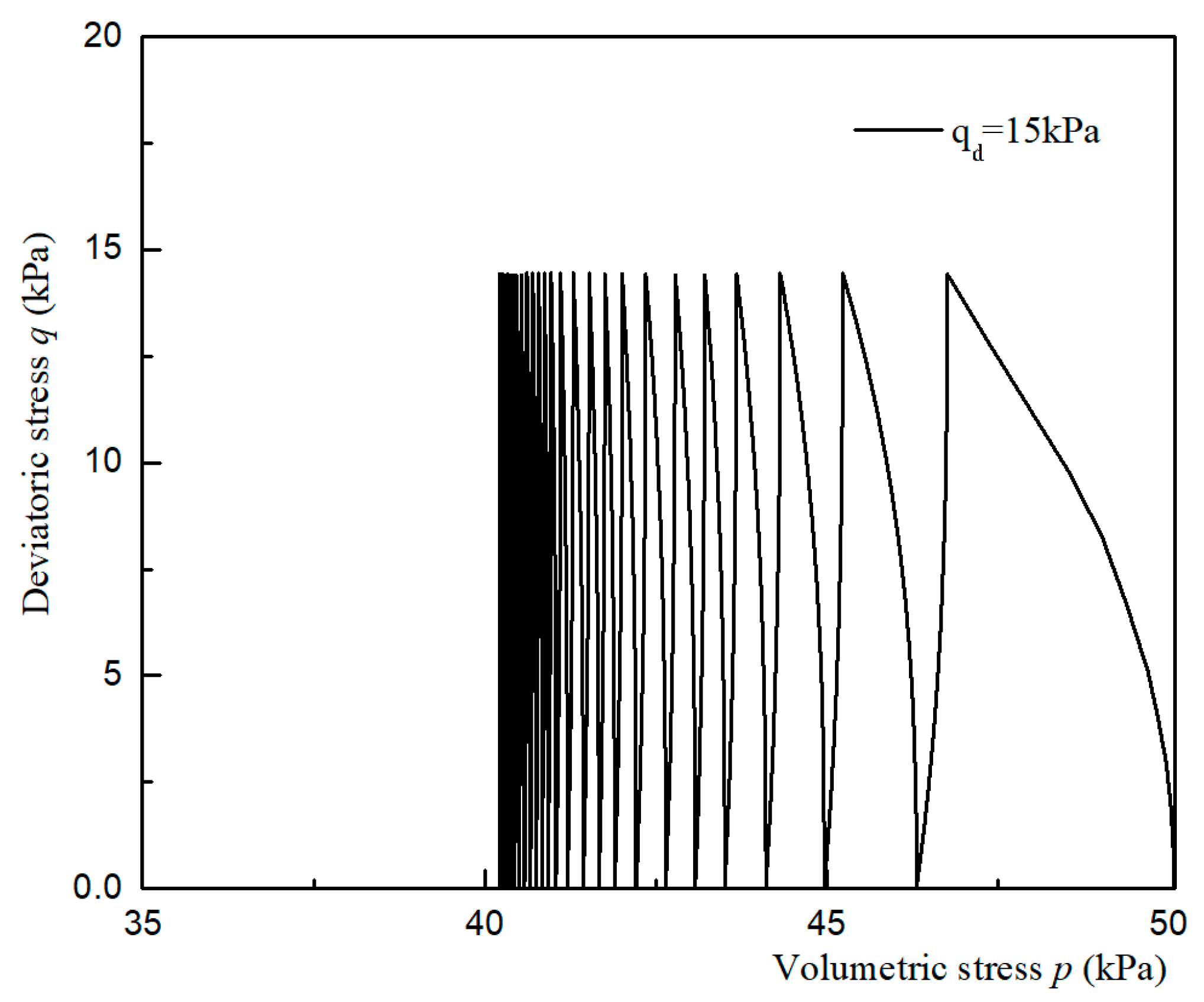
3. Verification of the Model
4. Numerical Results and Interpretations
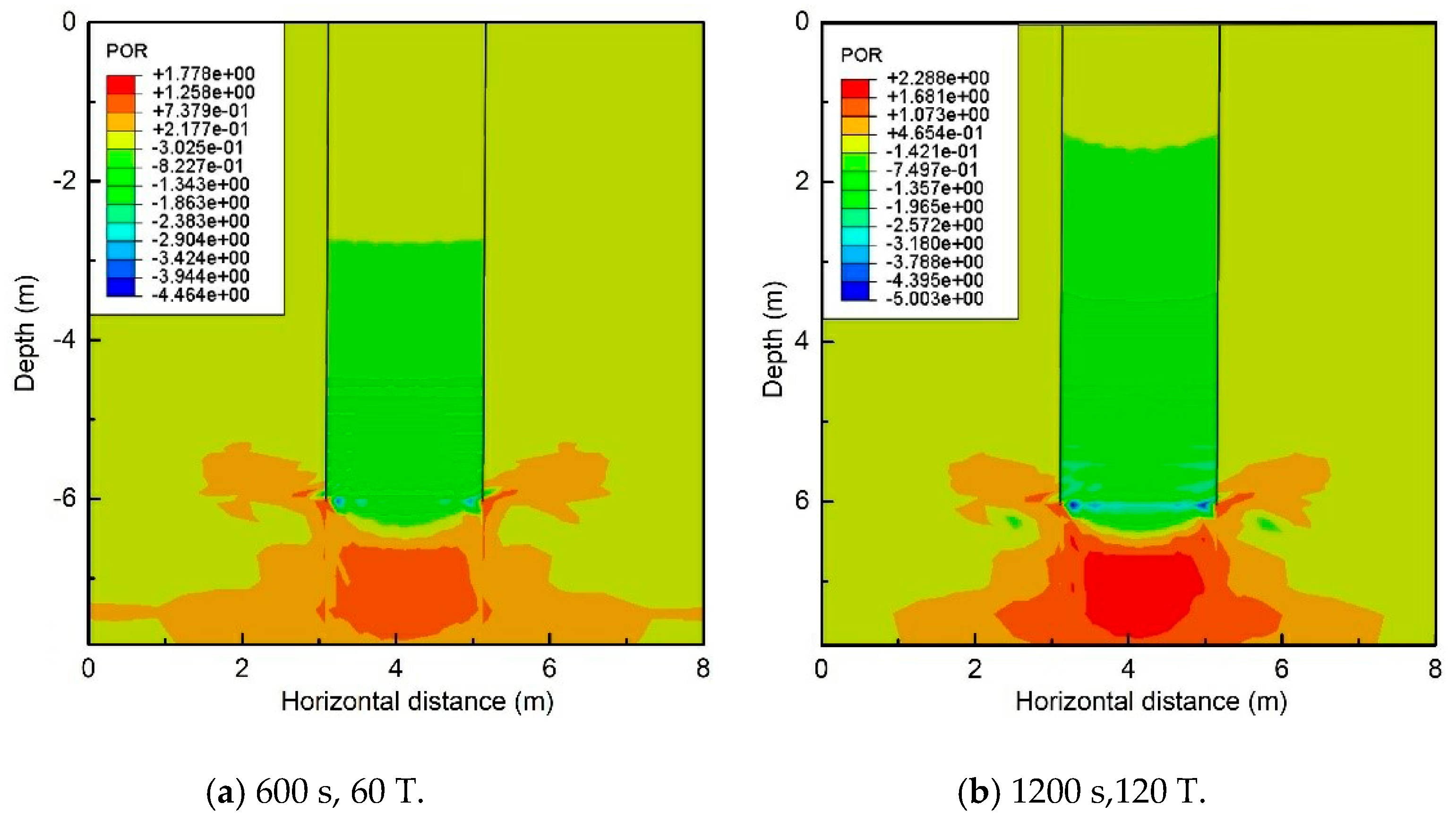
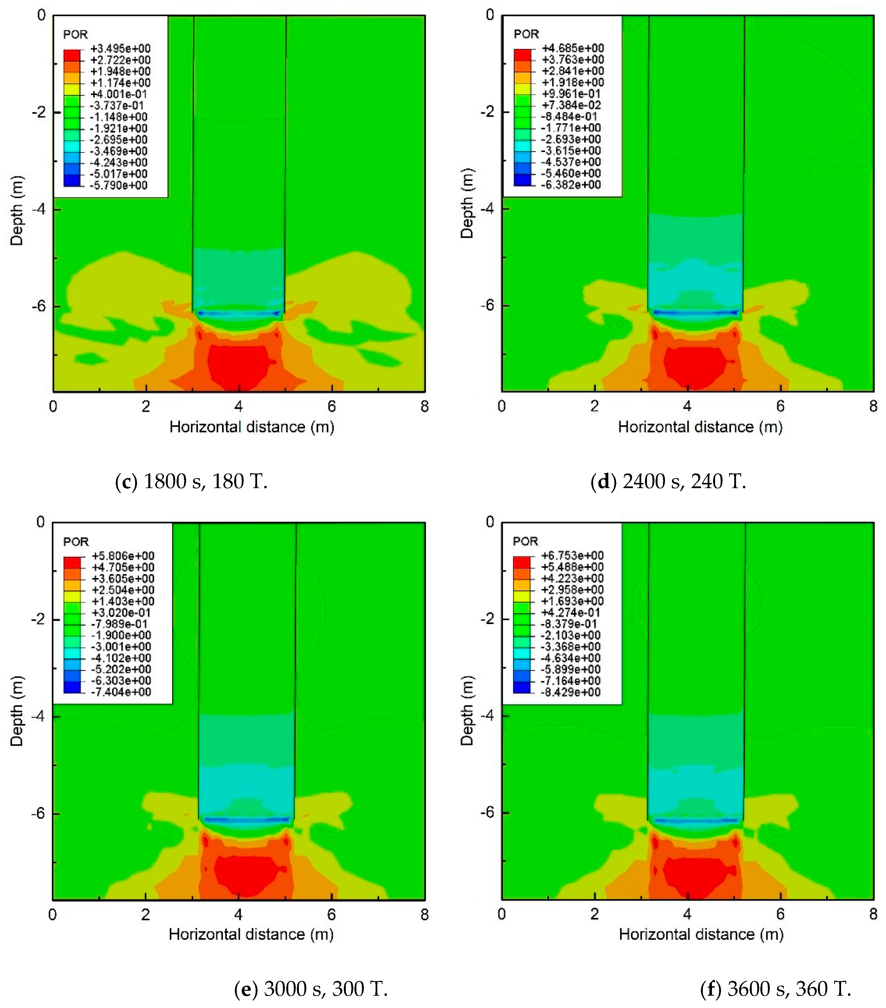
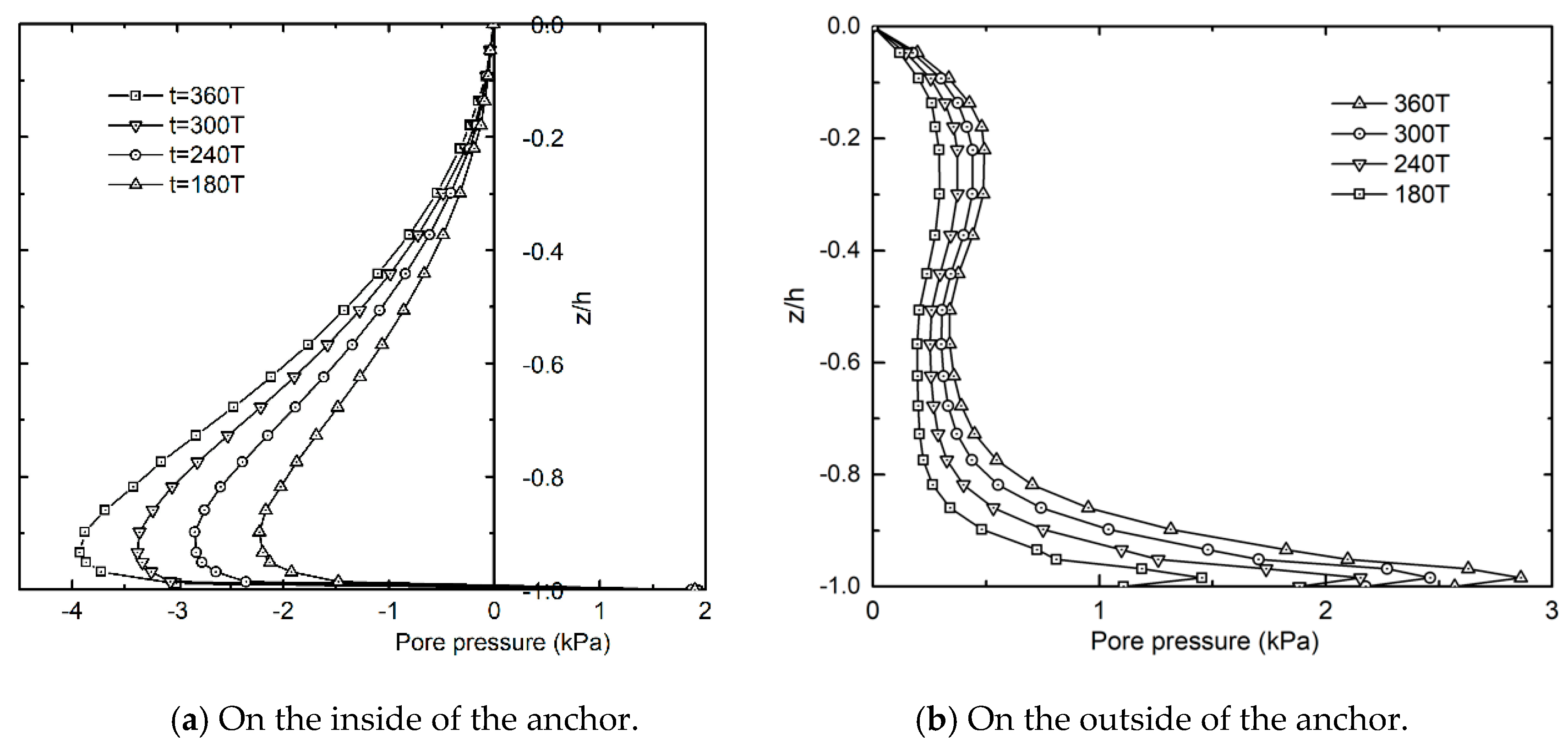
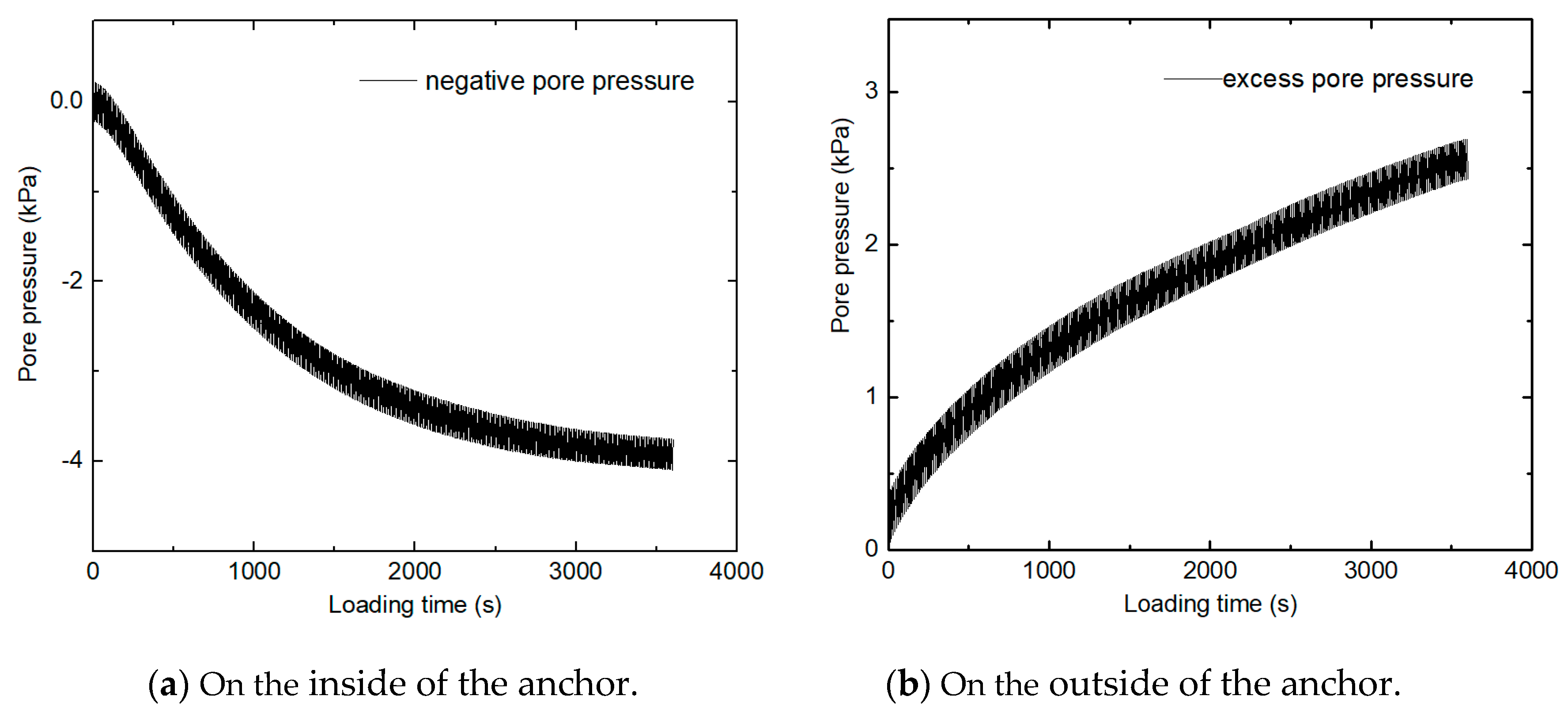
4.1. Accumulation of Pore Water Pressure Around the Suction Anchor
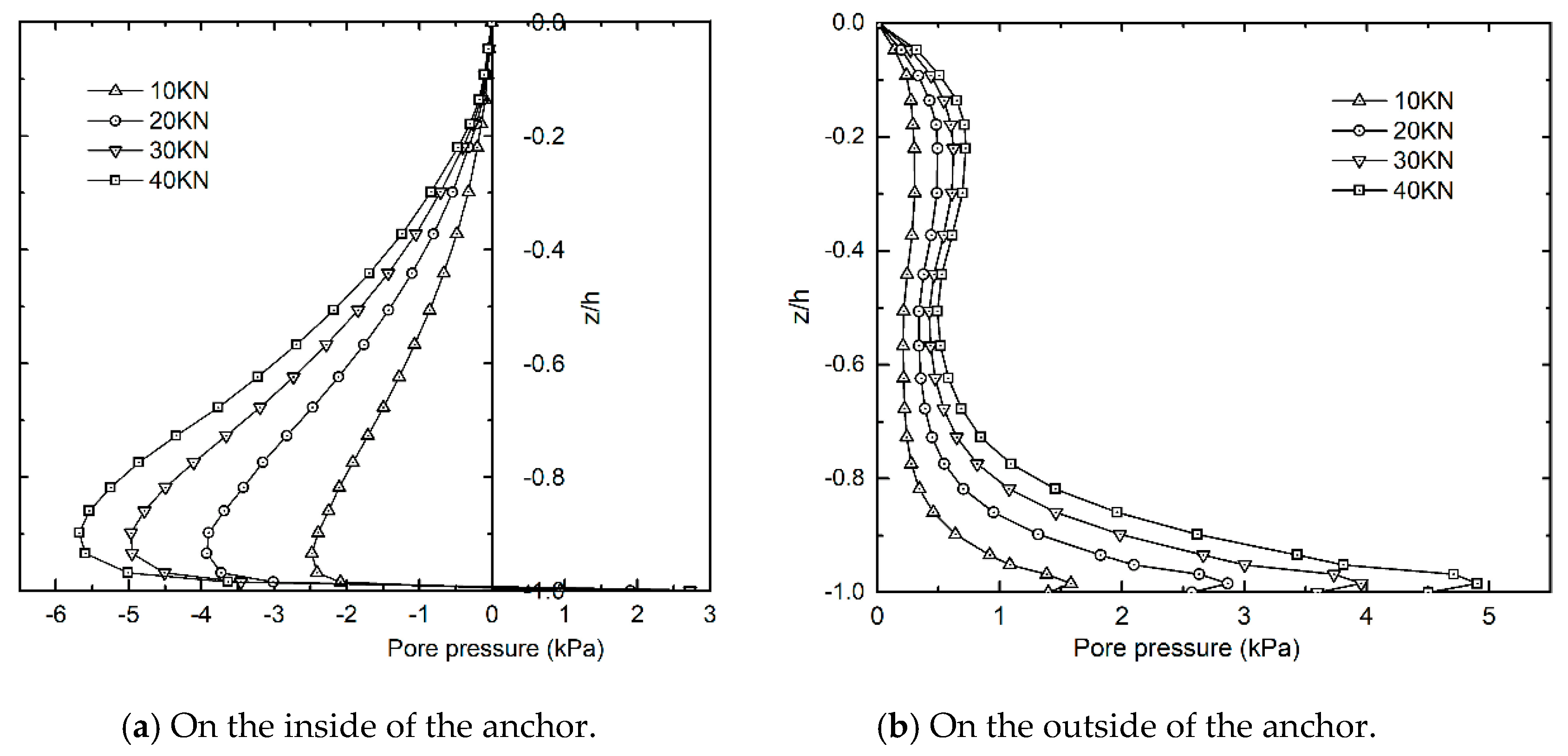
4.2. Effect of Load Amplitude
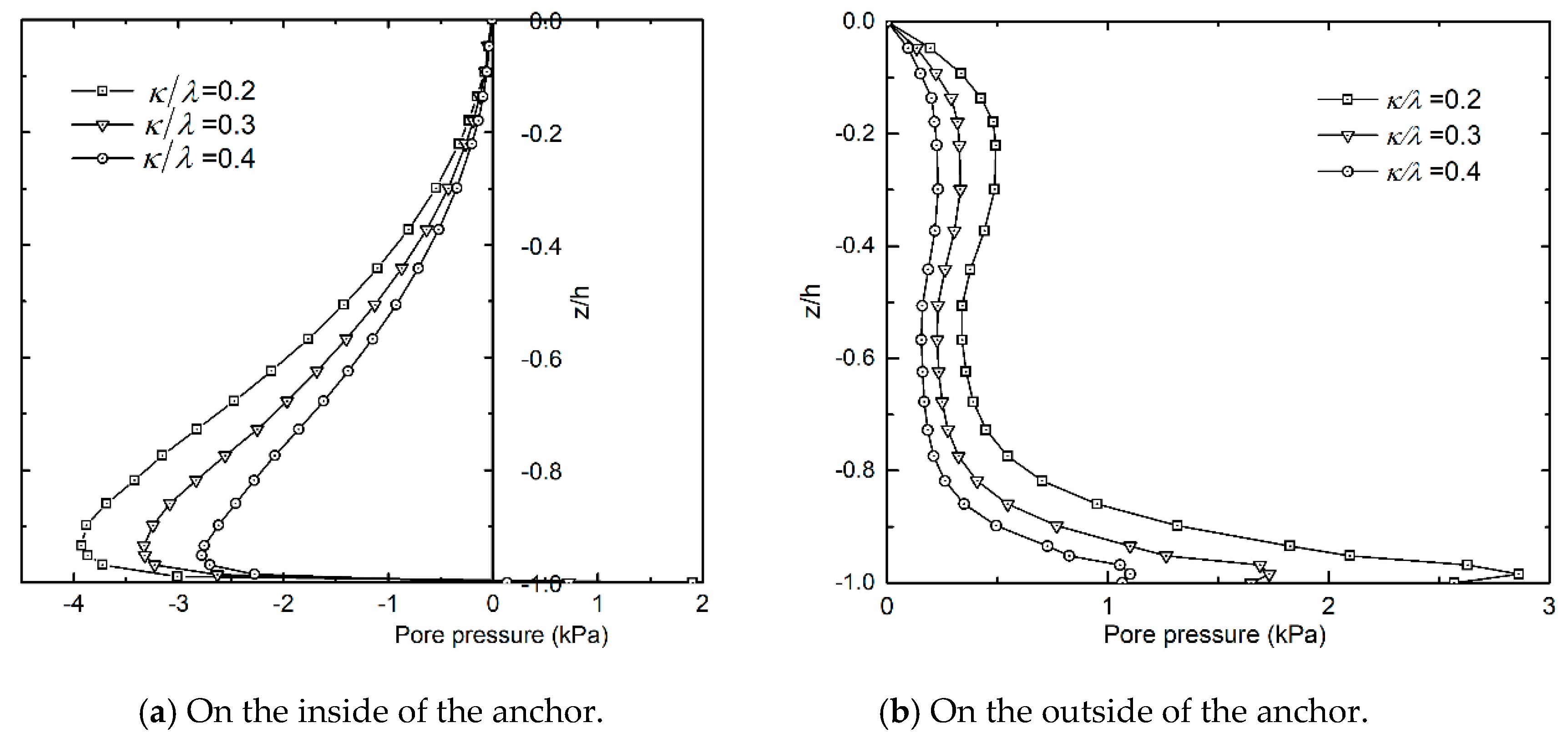
4.3. Effect of λ and κ
5. Perforated Suction Anchor
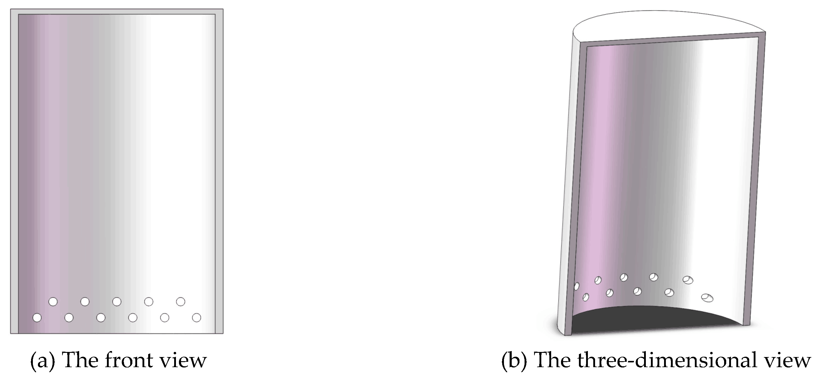
5.1. New Anchor Structure Style
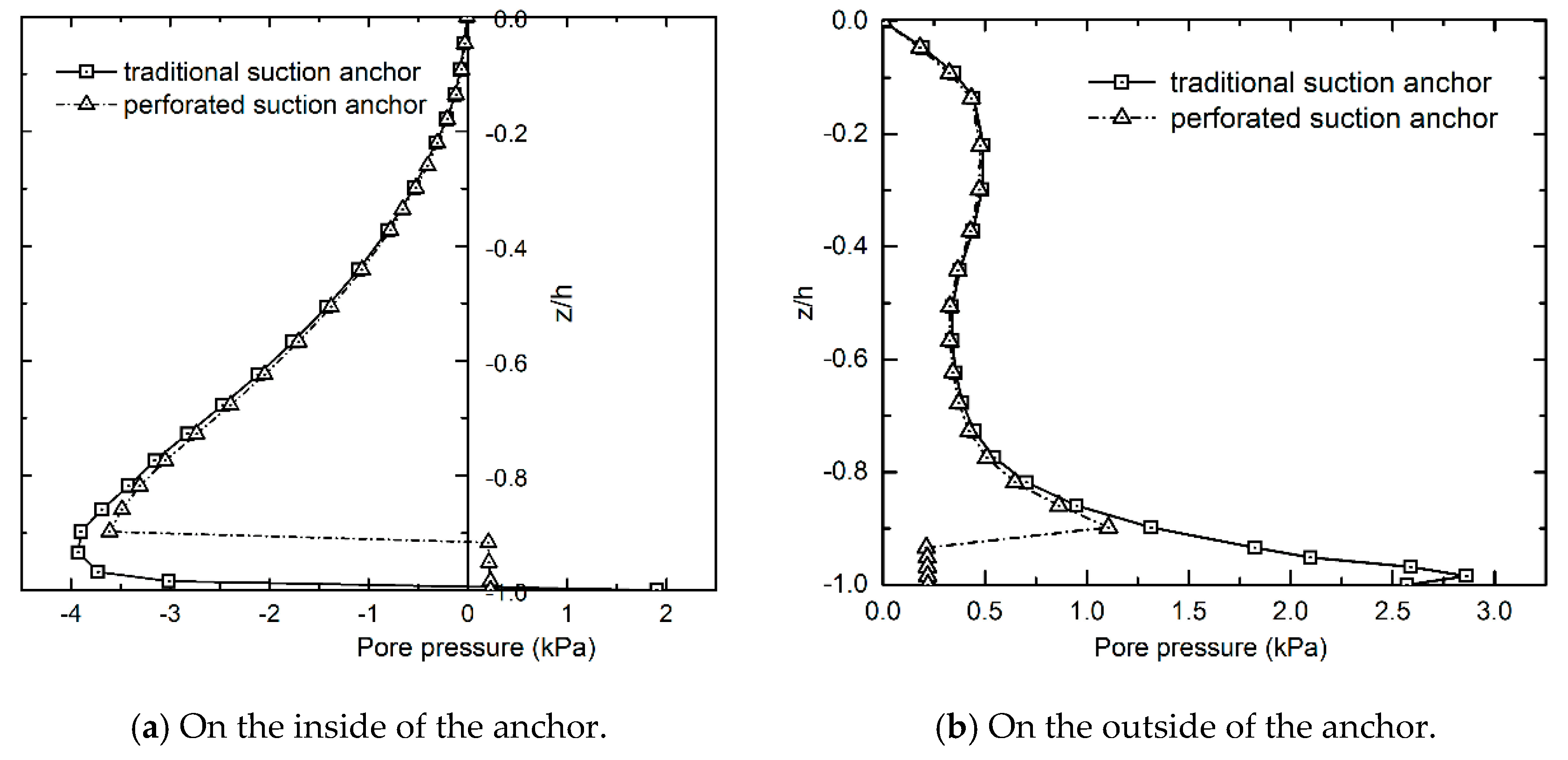
5.2. Comparative Study of the Pore Water Pressure Distribution
6. Concluding Remarks
- (1)
- A damage-dependent bounding surface model with combined isotropic-kinematic hardening rule was proposed to predict the accumulation of pore water pressure. The proposed model reasonably agreed well with the experiment result, against triaxial tests on anisotropically consolidated saturated clays and normally consolidated saturated clays. Thus the presented model was available to describe the key features of the cyclic behaviors of soft clay under cyclic loading conditions, including the pore water pressure response, accumulation of plastic deformation, and initial anisotropy.
- (2)
- Under the vertical cyclic loading condition, the excess pore water pressure primarily appeared on the outside of the suction anchor, and negative pore pressure mainly appeared on the inside, respectively. The maximum values on both sides appeared in the lower part of the seabed, due to the larger effective stress in the seabed soil, and these increased gradually with the loading time. The accumulation of excess pore water pressure can decrease the effective stress in the soil, and further reducing the uplift capacity of the suction anchor.
- (3)
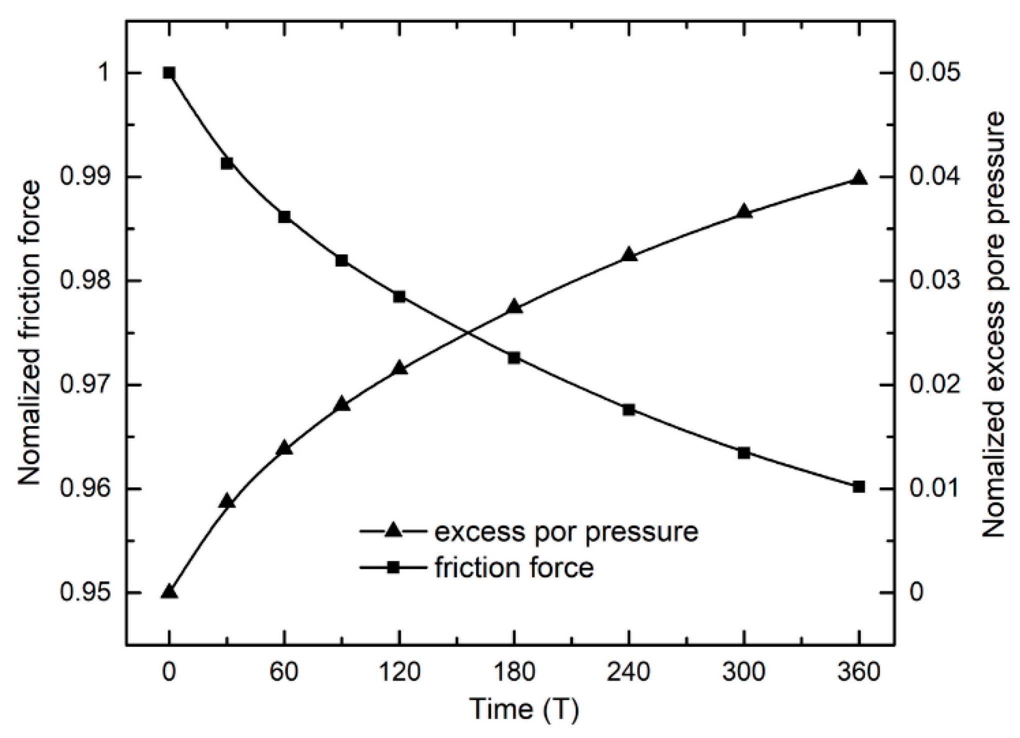
- According to the distribution characteristics of the residual pore pressure around the suction anchor, a new structure can reduce the accumulation of excess pore water pressure in the lower part of the seabed was proposed, which could increase external wall friction force under cyclic loading conditions. For the working conditions adopted in the present study, the new structure can reduce the excess pore water pressure by about 27.5%.
Author Contributions
Funding
Conflicts of Interest
References
- Andersen, K.H.; Dyvik, R.; Schroder, K.; Hansteen, O.E.; Bysveen, S. Field tests of anchors in clay II: Predictions and interpretation. J. Geotech. Eng. 1993, 119, 1532–1549. [Google Scholar] [CrossRef]
- Randolph, M.F.; Gaudin, C.; Gourvenec, S.M.; White, D.J.; Boylan, N.; Cassidy, M.J. Recent advances in offshore geotechnics for deep water oil and gas developments. Ocean Eng. 2011, 38, 818–834. [Google Scholar] [CrossRef]
- Moses, G.G.; Rao, S.N.; Rao, P.N. Undrained strength behaviour of a cemented marine clay under monotonic and cyclic loading. Ocean Eng. 2003, 30, 1765–1789. [Google Scholar] [CrossRef]
- Cheng, X.; Wang, J.; Wang, Z. Incremental elastoplastic FEM for simulating the deformation process of suction caissons subjected to cyclic loads in soft clays. Appl. Ocean Res. 2016, 59, 274–285. [Google Scholar] [CrossRef]
- Wallace, J.F.; Rutherford, C.J. Response of vertically loaded centrifuge suction caisson models in soft clay. In Proceedings of the Offshore Technology Conference, Houston, TX, USA, 1–4 May 2017. [Google Scholar]
- Dyvik, R.; Andersen, K.H.; Hansen, S.B.; Christophersen, H.P. Field tests of anchors in clay. I: Description. J. Geotech. Eng. 1993, 119, 1515–1531. [Google Scholar] [CrossRef]
- Tjelta, T.I.; Guttormsen, T.R.; Hermstad, J. Large-scale penetration test at a deepwater site. In Proceedings of the Offshore Technology Conference OTC 5103, Houston, TX, USA, 5–8 May 1986; pp. 201–212. [Google Scholar]
- Luke, A.M.; Rauch, A.F.; Olson, R.E.; Mecham, E.C. Components of suction caisson capacity measured in axial pullout tests. Ocean Eng. 2005, 32, 878–891. [Google Scholar] [CrossRef]
- Allersma, H.G.B.; Kierstein, A.A.; Maes, D. Centrifuge modelling on suction piles under cyclic and long term vertical loading. In Proceedings of the Tenth International Offshore and Polar Engineering Conference, Seattle, WA, USA, 28 May–2 June 2000. [Google Scholar]
- Mcmanus, K.J.; Kulhawy, F.H. Cyclic axial loading of drilled shafts in cohesive soil. J. Geotech. Eng. 1994, 120, 1481–1497. [Google Scholar] [CrossRef]
- Rao, S.N.; Ravi, R.; Prasad, B.S. Pullout behavior of suction anchors in soft marine clays. Mar. Georesources Geotechnol. 1997, 15, 95–114. [Google Scholar]
- Zhang, J.H.; Zhang, L.M.; Lu, X.B. Centrifuge modeling of suction bucket foundations for platforms under ice-sheet-induced cyclic lateral loadings. Ocean Eng. 2007, 34, 1069–1079. [Google Scholar] [CrossRef]
- Liao, C.; Chen, J. Accumulation of pore water pressure in a homogeneous sandy seabed around a rocking mono-pile subjected to wave loads. Ocean Eng. 2019, 173, 810–822. [Google Scholar] [CrossRef]
- Zhang, Y.; Ye, J.; He, K.; Chen, S. Seismic dynamics of pipeline buried in dense seabed foundation. Mar. Sci. Eng. 2019, 7, 190. [Google Scholar]
- Jeng, D.; Rahman, M.; Lee, T. Effects of inertia forces on wave-induced seabed response. Int. J. Offshore Polar Eng. 1999, 9, 307–313. [Google Scholar]
- Marin, M.; Craciun, E.M.; Pop, N. Considerations on mixed initial-boundary value problems for micopolar porous bodies. Dyn. Syst. Appl. 2016, 25, 175–195. [Google Scholar]
- Jeng, D.S.; Ye, J.H.; Zhang, J.S.; Liu, P.F. An integrated model for the wave-induced seabed response around marine structures: Model verifications and applications. Coast. Eng. 2013, 72, 1–19. [Google Scholar] [CrossRef]
- Duan, L.; Jeng, D.-S.; Liao, C.; Zhu, B.; Tong, D. A three-dimensional poro-elastic integrated model for wave and current-induced oscillatory soil liquefaction around an offshore pipeline. Appl. Ocean Res. 2017, 68, 293–306. [Google Scholar] [CrossRef]
- Duan, L.; Jeng, D. 2D numerical study of wave and current-induced oscillatory non-cohesive soil liquefaction around a partially buried pipeline in a trench. Ocean Eng. 2017, 135, 39–51. [Google Scholar] [CrossRef] [Green Version]
- Foo, C.S.X.; Liao, C.; Chen, J. Two-dimensional numerical study of seabed response around a buried pipeline under wave and current loading. J. Mar. Sci. Eng. 2019, 7, 66. [Google Scholar] [CrossRef]
- Cristescu, N.D. Mechanics of elastic composites. Math. Z. 2003, 258, 381–394. [Google Scholar]
- Shen, K.; Wang, L.; Guo, Z.; Jeng, D.S. Numerical investigations on pore-pressure response of suction anchors under cyclic tensile loadings. Eng. Geol. 2017, 227, 108–120. [Google Scholar] [CrossRef]
- Manzari, M.T.; Noor, M.A. On implicit integration of bounding surface plasticity models. Comput. Struct. 1997, 63, 385–395. [Google Scholar] [CrossRef]
- Liu, M.D.; Carter, J.P. A structured Cam Clay model. Can. Geotech. J. 2002, 39, 1313–1332. [Google Scholar] [CrossRef] [Green Version]
- Yu, H.S.; Khong, C.; Wang, J. A unified plasticity model for cyclic behavior of clay and sand. Mech. Res. Commun. 2007, 34, 97–114. [Google Scholar] [CrossRef]
- Hu, C.; Liu, H.; Huang, W. Anisotropic bounding-surface plasticity model for the cyclic shakedown and degradation of saturated clay. Comput. Geotech. 2012, 44, 34–47. [Google Scholar] [CrossRef]
- Dafalias, Y.F. An anisotropic critical state soil plasticity model. Mech. Res. Commun. 1986, 13, 341–347. [Google Scholar] [CrossRef]
- Dafalias, Y.F. On Cyclic and Anisotropic Plasticity: (1) A General Model Including Material Behavior Under Stress Reversals; (2) Anisotropic Hardening for Initially Orthotropic Materials. Ph.D. Thesis, University of California, Berkeley, CA, USA, 1975. [Google Scholar]
- Tao, L.; Meissner, H. Two-surface plasticity model for cyclic undrained behavior of clays. J. Geotech. Geoenviron. Eng. 2002, 128, 613–626. [Google Scholar]
- Yi, J.T.; Lee, F.H.; Goh, S.H.; Zhang, X.Y.; Wu, J.F. Eulerian finite element analysis of excess pore pressure generated by spudcan installation into soft clay. Comput. Geotech. 2012, 42, 157–170. [Google Scholar] [CrossRef]
- Stipho, A.S.A.Y. Experimental and Theoretical Investigation of the Behavior of Ansiotropically Consolidated Kaolin. Ph.D. Thesis, Cardiff University, Cardiff, UK, 1978. [Google Scholar]
- Zhong, H.H.; Huang, M.S.; Wu, S.M.; Zhang, Y.J. On the deformation of soft clay subjected to cyclic loading. Chin. J. Geotech. Eng. 2002, 24, 629–632. [Google Scholar]
- Cho, Y.; Lee, T.H.; Chung, E.S.; Bang, S. Field tests on pullout loading capacity of suction piles in clay. In Proceedings of the 22nd International Conference on Offshore Mechanics and Arctic Engineering, Cancun, Mexico, 8–13 June 2003; pp. 693–699. [Google Scholar]
- Steensen-Bach, J.D. Recent model tests with suction piles in clay and sand. In Proceedings of the Offshore Technology Conference, Houston, TX, USA, 4–7 May 1992. [Google Scholar]
- Mahmoodzadeh, H.; Randolph, M.F.; Wang, D. Numerical simulation of piezocone dissipation test in clays. Géotechnique 2014, 64, 657–666. [Google Scholar] [CrossRef]
- Schofield, A.N.; Wroth, C.P. Critical State Soil Mechanics; McGraw-Hill: London, UK, 1968. [Google Scholar]
- Chen, W.; Zhou, H.; Randolph, M.F. Effect of installation method on external shaft friction of caissons in soft clay. J. Geotech. Geoenviron. Eng. 2009, 135, 605–615. [Google Scholar] [CrossRef]
- Andersen, K.H.; Murff, J.D.; Randolph, M.F. Suction anchors for deepwater applications. In Proceedings of the International Symposium on Frontiers in Offshore Geotechnics, Perth, WA, Australia, 19–21 September 2005. [Google Scholar]


| Effective Unit Weight (kN/m3) | Compression Index (λ) | Swelling Index (κ) | Poisson’s Ratio (ν) | Permeability Coefficient (m/s) | |
|---|---|---|---|---|---|
| 7.17 | 0.17 | 0.34 | 0.3 | 0.62 | |
| β | |||||
| 1.72 | 3.5 | 120 | 0.5 |
| Parameters | Kaolin Clay (Stipho) | Kaolin Clay (Tao) | Soft Clay (Zhong) |
|---|---|---|---|
| Slope of critical state line (M) | 1.12 | 1.1 | 1.15 |
| Compression index (λ) | 0.14 | 0.17 | 0.25 |
| Swelling index (κ) | 0.05 | 0.34 | 0.05 |
| Effective Poisson’s ratio (ν) | 0.2 | 0.3 | 0.25 |
| 2 | 1.72 | 1.5 | |
| - | 3.5 | 6 | |
| - | 120 | 40 | |
| β | - | 0.5 | 1.5 |
© 2019 by the authors. Licensee MDPI, Basel, Switzerland. This article is an open access article distributed under the terms and conditions of the Creative Commons Attribution (CC BY) license (http://creativecommons.org/licenses/by/4.0/).
Share and Cite
Li, H.; Chen, X.; Hu, C.; Wang, S.; Liu, J. Accumulation of Pore Pressure in a Soft Clay Seabed around a Suction Anchor Subjected to Cyclic Loads. J. Mar. Sci. Eng. 2019, 7, 308. https://doi.org/10.3390/jmse7090308
Li H, Chen X, Hu C, Wang S, Liu J. Accumulation of Pore Pressure in a Soft Clay Seabed around a Suction Anchor Subjected to Cyclic Loads. Journal of Marine Science and Engineering. 2019; 7(9):308. https://doi.org/10.3390/jmse7090308
Chicago/Turabian StyleLi, Hui, Xuguang Chen, Cun Hu, Shuqing Wang, and Jinzhong Liu. 2019. "Accumulation of Pore Pressure in a Soft Clay Seabed around a Suction Anchor Subjected to Cyclic Loads" Journal of Marine Science and Engineering 7, no. 9: 308. https://doi.org/10.3390/jmse7090308