A Wave Energy Converter Design Load Case Study

Abstract

This article presents an example by which design loads for a wave energy converter (WEC) might be estimated through the various stages of the WEC design process. Unlike previous studies, this study considers structural loads, for which, an accurate assessment is crucial to the optimization and survival of a WEC. Three levels of computational fidelity are considered. The first set of design load approximations are made using a potential flow frequency-domain boundary-element method with generalized body modes. The second set of design load approximations are made using a modified version of the linear-based time-domain code WEC-Sim. The final set of design load simulations are realized using computational fluid dynamics coupled with finite element analysis to evaluate the WEC’s loads in response to both regular and focused waves. This study demonstrates an efficient framework for evaluating loads through each of the design stages. In comparison with experimental and high-fidelity simulation results, the linear-based methods can roughly approximate the design loads and the sea states at which they occur. The high-fidelity simulations for regular wave responses correspond well with experimental data and appear to provide reliable design load data. The high-fidelity simulations of focused waves, however, result in highly nonlinear interactions that are not predicted by the linear-based most-likely extreme response design load method.

1. Introduction

The structural requirements necessary to ensure the survival of a wave energy converter (WEC) in extreme sea states are a key cost driver in WEC design and represent a central challenge to the development of WECs into a reliable, cost-efficient source of renewable energy. To optimize a WEC’s structural design, considering both performance and cost, it is essential to incorporate structural analyses with traditional hydrodynamic analyses throughout the entire design process. The largest loads that a WEC system/component will be subject to throughout its design life are typically referred to as the design loads. An accurate evaluation of the design loads should ensure WEC survival, make possible an optimized system design, and minimize overall WEC costs.

Typically, offshore design loads are evaluated using a site-specific joint probability distribution for significant wave heights (H_s), wave energy periods (T_e), as well as, possibly, wave direction, spectral shape, wind speed, and wind direction. Extreme sea-state probabilities within the joint probability distribution are usually specified with typical return period contours, such as 25, 50, or 100 years. As reviewed in [1,2], for a specified wave environment and design life, there are several possible approaches to calculating design loads. The simplest method is the one-dimensional design load approach, where loads are assessed at the maximum H_s on the designated design life/return period contour for a range of T_e, and the maximum resulting load is selected as the design load [3,4]. Similarly, a contour design load method may be used, where the response loads are instead calculated at intervals along the design life/return period contour, and the maximum resulting load is, again, taken as the design load [4,5]. However, the largest loads (i.e., design loads) are not always caused by the largest waves; they may instead be a result of the instantaneous position of the WEC after a particular series of irregular waves. Consequently, an all-sea-state approach (which may also be referred to as the full long-term approach) is the most accurate method for assessing WEC design loads [4,5]. Using the all-sea-state approach, short-term extreme responses are first calculated at sea states throughout the entire (H_s, T_e) joint probability distribution, where a 3-h duration is typically used to define the short-term response. The short-term response distributions are then scaled by their probability of occurrence and integrated across the joint probability distribution to obtain the long-term design load at the specified design life.

Although the applied design load methodology specifies which sea states are considered in evaluating the design loads, it does not stipulate how the stochastic sea states should be realized. A site-specific wave spectrum, either idealized or empirical, is typically used to quantify irregular ocean waves. For numerical simulations, the wave spectrum may be used to generate a time series of irregular waves for the specified timeframe. However, for typical simulation times of 3 h or more, this approach is often too computationally intensive, especially for high-fidelity models. To reduce the timeframe of interest, it is common to assume that the wave heights for a specified sea state follow a Rayleigh distribution. Using this approximation, the extreme wave heights may then be estimated using regular wave heights equal to H = 1.9 H_s [5]. Another approach to reducing the simulation timeframe is the use of an equivalent design, or focused wave. Using this approach, a series of waves are identified that will generate the most-likely extreme wave or WEC response for a specified sea state [6].

Regardless of the design load methodology and the sea-state realization methodology utilized, a modeling approach must also be selected to simulate the waves and the WEC’s responses. There is a broad range of modeling approaches available, many of which were originally developed for ship and offshore oil and gas platform design. The linear frequency-domain boundary-element method (BEM) (e.g., WAMIT [7] and Nemoh [8]), which is based on potential flow theory and a linearized free surface condition, is the simplest modeling approach, with the lowest level of computational fidelity. Using radiation and diffraction theory, BEM codes can compute the hydrodynamic loads, hydrodynamic coefficients, and system dynamics in the frequency domain. To evaluate structural deformations and loads using a BEM-based code, the generalized body-modes methodology is used in conjunction with the linear hydrodynamic analysis [9,10]. Because BEM codes solve the system dynamics directly in the frequency domain, the simulation time is orders of magnitude less than real time. Using BEM-generated hydrodynamic coefficients, the WEC system dynamics can also be solved in the time domain (e.g., WEC-Sim [11]). Using this approach, additional forcing terms may also be considered, such as quadratic damping, nonlinear restoring and Froude–Krylov forces, multibody dynamics, power take-off and control system forces, dynamic mooring loads, and generalized body–mode interactions [12]; consequently, higher simulation fidelities are possible. Simulation times for the BEM-based time-domain-type codes are normally on the order of real time, but increase significantly when additional forcing terms are considered, particularly the nonlinear restoring and Froude–Krylov forces. To model highly nonlinear wave-structure-interaction effects, such as finite amplitude motion, turbulence, boundary-layer viscous flow separation, overtopping, and wave breaking, models based on the Reynolds-averaged Navier–Stokes (RANS) equations, rather than potential flow theory, must be used. For structural load evaluations, the RANS computational fluid dynamics (CFD) solver must also be coupled with a finite element analysis (FEA) solver, or similar, either using one-way coupling or two-way coupling, depending on the level of fluid-structure-interaction. High-fidelity RANS and FEA codes have a large span of simulation times, roughly 10⁴ to 10⁸ times real time, depending on the computational resources available and the model complexity.

Each potential combination of the design load method, sea-state realization method, and modeling method is valid; however, this should be carefully selected based on the computational resources available and the design stage. In the early stages of a WEC design, in which many proof-of-concept estimates and iterative design optimizations are typically conducted, a lower-fidelity, computationally efficient approach should be used. When at the later stages of design, a limited number of high-fidelity, computationally intensive simulations will likely be necessary to verify the extreme loads and ensure the survival of the WEC through its design life. Additionally, experimental testing (usually at a reduced scale) and empirically based models are also typically necessary throughout the design process to provide both load predictions and numerical model validation.

This study presents an example of a computationally efficient framework for evaluating the structural design loads of a WEC, from the conceptual design stages to the final design stages. Existing WEC design guidelines are applied in these analyses, where they are available [1,3,4,5]. The WEC selected for this case study is Reference Model 3 (RM3), a two-body floating-point absorber WEC [13,14]. The loads evaluated are the spar axial force (F_axial), the spar bending moment (M_spar), and the mooring line force (F_mooring). Three design stages are considered; the modeling results of each preceding stage are used as a basis for the subsequent, higher-fidelity modeling stage. The first set of design load evaluations are obtained using WAMIT, a frequency-domain BEM code. The second set of design load evaluations are made using WEC-Sim with the application of the generalized body-modes method. The final design load calculations are carried out using CFDs coupled with FEA to simulate the load responses to both regular and focused waves.

2. Materials and Methods

2.1. Reference Model 3 Wave Energy Converter

For this case study, the RM3 WEC was used to demonstrate the design load evaluation framework [13]. RM3 is one of the U.S. Department of Energy WEC reference models [14], and consequently, experimental results are available for validating numerical models and simulations. The 1:100-scale version of the RM3 model was used in this study, because this is the scale at which the extreme condition wave tests were carried out. The 1:100-scale RM3 model is pictured in Figure 1, and the model properties are listed in

Table 1. RM3 1:100-scale model properties [13].

Property	Value	Units
m	0.313	kg
Ix	8.89 × 10−3	kg·m2
Iy	8.89 × 10−3	kg·m2
zcg	−0.214	m
zmooring,top	−0.051	m
zmooring,bottom	−0.213	m
kmooring	0.700	N/m

. Two sets of four mooring lines, for a total of eight lines, each with a stiffness of 0.7 N/m, were used during these tests. A complete description of the test article and the tank test settings are documented in [13]. Responses to regular waves, with full-scale wave heights of roughly 3, 9, 15, and 18 m, were evaluated during these tests, with surge, heave, pitch, and axial spar force responses recorded. The spar forces were assessed with a force transducer between the spar plate and the float; the bending moments and mooring line forces, however, were not measured.

2.2. Environmental Conditions

The joint probability distribution assumed for this study, as plotted in Figure 2, is based on measurements obtained near Humboldt Bay, California, as recorded by the National Data Buoy Center Buoy 46022. For these data, the WEC design response toolbox [15,16] was used to calculate the design life/return contours shown in Figure 2, using the principle component contour method [17]. The regular wave, full-scale experimental tank test conditions [13] are also plotted in Figure 2; from which it can be seen that the nominally 15-m tank test data roughly approximate a one-dimensional design load evaluation method (15 m ÷ 1.9 = 7.89 m ≈ 1 year H_s,max). Consequently, for the purpose of model validation, and as a relevant timeframe for a demonstration deployment, 1 year was used as the design life in the following studies.

2.3. Design Load Analyses

The subsequent studies demonstrate one possible framework for evaluating WEC structural design loads, from the early to the final design stages. Three modeling approaches were used. The first set of design load approximations were calculated using BEM theory. The second set of design load estimates were obtained using a modified version of the linear-based time-domain code WEC-Sim. The final evaluations were accomplished using both regular and most-likely extreme response (MLER) design waves in CFD coupled with FEA. The following data and results are reported at full scale, unless otherwise indicated. For comparison purposes, F_axial and M_spar were calculated at the 1:100-scale model transducer location (z = −0.311 m); and for simplicity, only F_mooring for one of the top level, upstream lines is reported, where x–z plane symmetry was assumed in all models.

2.3.1. WAMIT Simulations

WAMIT (WAMIT v7, WAMIT Inc., Chestnut Hill, MA, USA) is the BEM code used in this study for both the hydrodynamic and generalized body-modes analyses. Because the generalized body-mode amplitudes are several orders of magnitude smaller than the rigid body displacements, RM3 is modeled at full scale in WAMIT to minimize numerical error and improve convergence. As illustrated in Figure 3a, the full-scale RM3 WAMIT model uses an average sized panel of 0.26 m × 0.26 m, resulting in a total of 13,800 panels. As described in the WAMIT user manual [7], structural deformations were considered using a set of corresponding vibration modes, which are treated as additional degrees of freedom (DOF) to the standard six rigid-body DOFs. Each additional generalized body-mode DOF is defined with the specification of a normalized mode shape, X_i, and the associated modal mass, M_i, and stiffness, K_i. As described in [18], using the Rayleigh–Ritz method, these mode shapes, mass, and stiffness matrices may be calculated by approximating the RM3 model as a beam with point masses representative of the float and spar, at their centers of mass, and discrete springs representative of the mooring system, as illustrated in Figure 3b. Based on previous evaluations [9,10], the first mode shape typically dominates the response. Consequently, for simplicity and with the goal of obtaining a first-order accurate solution from WAMIT, only the first mode shape of each type was considered. The normalized first axial (longitudinal oscillations) and bending (transverse oscillations) mode shapes, in terms of the normalized beam length, $\overline{x}=z/L_{draft}$, as well as the modal masses and stiffnesses are given in Figure 3c,d. With these model inputs, WAMIT was run for all relevant frequencies and the linear radiation and diffraction hydrodynamic coefficients (as will be applied later in WEC-Sim) were obtained for all rigid-body and generalized body-mode degrees of freedom.

To approximate the design loads using the WAMIT model, response amplitude operators (RAOs) were also calculated in WAMIT for each load of interest. For the WAMIT RAO calculations, the mooring system was modeled as an additional linear stiffness term and the viscous damping force was approximated as an additional linear damping term, applied to the rigid body degrees of freedom in the WAMIT BEM system of equations. To calculate 3-h short-term and 1-year long-term loads from the WAMIT RAO results, the process suggested by Faltinsen [19] was used. After discretizing the joint probability distribution pictured in Figure 2 into $18\times 18$ (T_e, H_s) sea-state bins, the variance of the response, ${\sigma }_r^2$, was approximated using Equation (1) for each sea state:

$${\sigma }_r^2={{\displaystyle \int }}_0^{\infty }S\left(\omega \right){\left|H\left(\omega \right)\right|}^{2}d\omega .$$

(1)

In Equation (1), S(ω) is the sea spectrum and H(ω) is the response transfer function (i.e., RAO). The Bretschneider spectrum was used for S(ω) in these calculations, as well as in the following WEC-Sim- and CFD-FEA-focused wave simulations. Assuming that the response peak probability density function can be approximated with a Rayleigh function, the most likely maximum short-term response, R_max, can then be calculated with Equation (2):

$$R_{max}={\left(2{\sigma }_r^2\log \left(t/T\right)\right)}^{1/2},$$

(2)

where T is the mean wave period and t, the short-term timeframe of interest, is specified as 3 h. The resulting short-term maximum responses, R_max, for F_axial, M_spar, and F_mooring, as calculated with Equation (2) for each sea state, are presented in Figure 9a,c,e, respectively, where they are compared with the WEC-Sim results.

The long-term probability level, Q, that the maximum response exceeds R was obtained with the summation across the joint probability distribution, given in Equation (3):

$$Q\left(R\right)={{\displaystyle \sum }}_{j=1}^{18}{{\displaystyle \sum }}_{k=1}^{18}exp\left(-0.5R^2/{\sigma }_{r,jk}^2\right)p_{jk},$$

(3)

where p_jk is the joint probability for each sea-state significant wave height (j) and period (k). The long-term design loads for F_axial, M_spar, F_mooring, as calculated with Equation (3), are given in Figure 10, where they are compared to the WEC-Sim results.

2.3.2. WEC-Sim Simulations

The second set of design load evaluations were calculated using the linear-based time-domain code WEC-Sim (v3.1) [11,12], in which irregular sea states and RM3 responses were simulated and statistically representative design loads were computed. WEC-Sim is an open-source collaboration between the National Renewable Energy Laboratory in Golden, CO, USA, and Sandia National Laboratories in Albuquerque, NM, USA, funded by the U.S. Department of Energy’s Water Power Technologies Office. WEC-Sim uses the hydrodynamic coefficients obtained from the BEM WAMIT model to solve the equation of motion for each body in the time domain based on Cummins’s equation [20]. This equation of motion for a floating-body system, where each body’s position is defined relative to its center of gravity, is given in Equation (4):

$$\left(m+m_{\infty }\right)\ddot{x}=-{{\displaystyle \int }}_{-\infty }^{t}K\left(t-\tau \right)\dot{x}\left(\tau \right)d\tau +F_e-F_{hs}+F_v+F_{ext}.$$

(4)

In Equation (4), m is the mass matrix; $m_{\infty }$ is the added mass matrix at infinite frequency; x is the position vector; K is the impulse response function; the term, ${{\displaystyle \int }}_{-\infty }^{t}K\left(t-\tau \right)\dot{x}\left(\tau \right)d\tau$, is the convolution integral, which represents the resistive force on the body caused by wave radiation; F_e is the wave-excitation force; F_hs is the hydrostatic restoring force; F_v is the viscous drag force; and F_ext includes any additional external forces. These external forces may include forces from power take-off mechanisms, mooring systems, and so on. The linear force coefficients, $m_{\infty }$, K, F_hs, and F_e, were obtained from the previously discussed WAMIT model.

The WEC-Sim model created for this study (shown in Figure 4) utilizes prebuilt blocks. However, the hydrodynamic body block, which includes components to calculate the wave radiation, excitation, hydrostatic restoring, viscous drag, and mooring forces, was modified, as described in [12], to include the hydrodynamic coefficients and solve Equation (4) for the generalized body-mode DOFs in addition to the standard six rigid-body DOFs.

In addition to the WAMIT-derived linear hydrodynamic coefficients, WEC-Sim requires inputs for the viscous drag coefficients, C_D, for each body and DOF. Heave, surge, and pitch, C_D, have been calculated in a previous study [2] for the 1:100-scale RM3 model using forced-oscillation CFD simulations in STAR-CCM+. The C_D values, as implemented in WEC-Sim, were 2.56 for surge (A_ref = 9.85 × 10⁻³ m²), 3.21 for heave (A_ref = 2.75 × 10⁻² m²), and 2.17 for pitch (A_ref = 2.50 × 10⁻⁵ m⁵).

Mooring forces in WEC-Sim may be modeled using either a simple spring matrix or by coupling WEC-Sim to the open-source code MoorDyn [21]. MoorDyn is a lumped-mass mooring line model, which allows arbitrary line interconnections with different line properties, clump weights, and floats. The model accounts for the mooring lines’ internal axial stiffness and damping, weight, and buoyancy forces, and hydrodynamic forces using Morison’s equation. Because of the two-layer mooring system, and because the mooring line mass and viscous drag forces relative to the 1:100-scale RM3 experimental model are non-negligible, the mooring configuration cannot be accurately described with a simple linear spring matrix in this case, and the MoorDyn model was used for these simulations.

Using the described WEC-Sim inputs and model setup, time-varying irregular wave forces were applied. The equations of motion were solved in the time domain for the RM3 body using a fourth-order, time-marching Runge–Kutta algorithm to obtain the system’s dynamic response. For the $18\times 18$ (T_e, H_s) discretized joint probability distribution, there were 201 sea states with a non-zero probability. For each of these sea states, six 3-h irregular wave realizations were run for a total of 18 h each, as recommended in [3]. For each simulation, a time step size of $dt=T_p/600$ was used, where $T_p\approx 1.1667T_e$ for the Bretschneider spectrum, and a startup ramp of $60T_p$ was used for the time-varying wave forces.

Using the resulting WEC-Sim-predicted time responses for F_axial, M_spar, and F_mooring, 3-h short-term extreme loads and 1-year long-term extreme loads were then calculated. The short-term extreme loads were calculated by fitting a Weibull cumulative distribution function (CDF) to the upper 80% percentile of the simulated empirical response peak CDF (i.e., a Weibull tail-fit), as detailed in [15,22]. From the Weibull CDF, the short-term extreme distribution function for a 3-h timeframe was then obtained, on which the short-term extreme load was identified as the load at the 90% percentile. The WEC-Sim-derived 3-h extreme loads for F_axial, M_spar, and F_mooring for each of the 201 sea states are presented in Figure 9b,d,f, where they are compared with the WAMIT-predicted 3-h extreme loads. The largest short-term extreme loads within the 1-year return contour, and the sea states where they occur, are noted in Figure 9. As described in [15,23], the all-sea-state long-term design loads were computed using the complementary cumulative distribution function:

$$CCDF=1-{{\displaystyle \sum }}_{j=1}^{18}{{\displaystyle \sum }}_{k=1}^{18}CDF·p_{jk},$$

(5)

a summation of the 201 probability weighted Weibull CDF fits. The ensuing long-term design loads for F_axial, M_spar, and F_mooring are plotted in Figure 10, where they are compared with the WAMIT-based results.

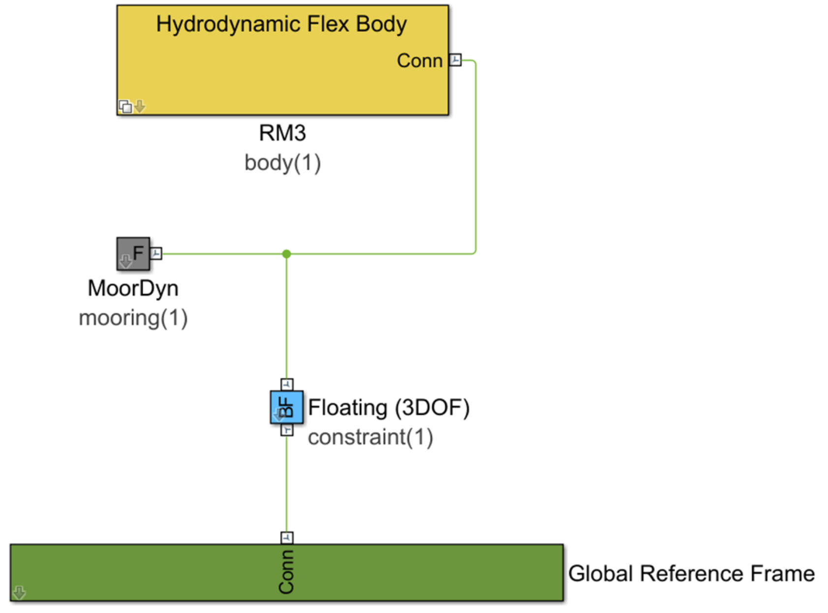
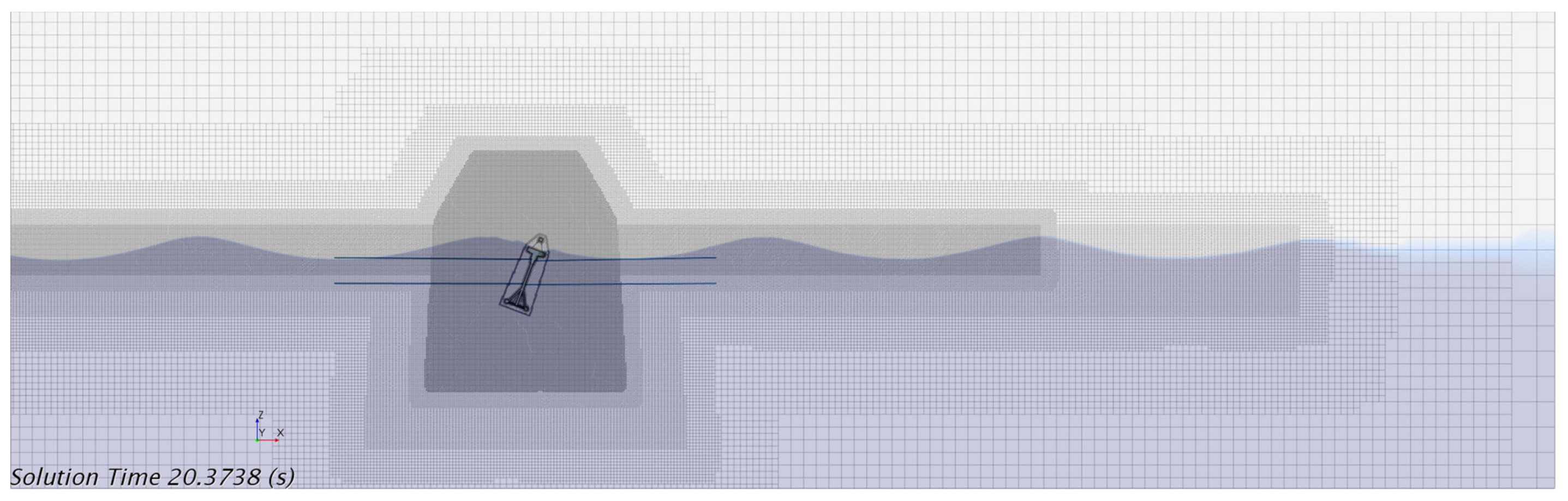
2.3.3. STAR-CCM+ Simulations

The final design load calculations were made using CFD coupled with FEA to simulate responses to both regular waves and MLER-focused waves. STAR-CCM+ (STAR-CCM+ v13.06.012, Siemens, Plano, TX, USA) [24] was used for both the CFD and FEA simulations. The CFD-FEA simulations were based on the 1:100-scale model and experimental tank parameters [13].

All of the CFD simulations were run using an unsteady, implicit RANS model with the SST k-ω turbulence model and all-y+ wall treatment. The SST k-ω closure model, which is based on the k-ω model near the wall region and the k-ε model in the free stream, was selected, since this formulation reduces the individual limitations of the k-ω model, which is sensitive to the initial conditions and convergence criteria, and the k-ε model, which is inaccurate for adverse pressure gradients and no-slip walls. As such, the SST k-ω turbulence model is a good compromise of computational stability, cost, and accuracy between the simpler RANS turbulence models and the more complex LES (large eddy simulation) turbulence models for capturing nonlinear viscous flow effects. All-y+ wall treatment was used to model the turbulence parameters in the wall boundary layer due to its adaptability and accuracy from the refined mesh sizes in the viscous sublayer to the course mesh sizes in the outer boundary layer, as well as the intermediate region.

The STAR-CCM+ fluid properties are listed in

Table 2. STAR-CCM+ model fluid properties.

Parameter	Setting	Units
ρwater	1000	kg/m3
μwater	8.887 × 10−4	Pa·s
ρair	1.184	kg/m3
μair	1.855 × 10−5	Pa·s

, where the Eulerian multiphase volume of fluid method was used to simulate the free surface. To model the large amplitude extreme wave motions as well as the mooring dynamics using a reasonably sized grid, STAR-CCM+’s overset mesh method was also used. The mooring line load (F_mooring) for each individual mooring line was modeled using a simple linear spring coupling with pretension and no repelling force. To model the structural loads (F_axial and M_spar), a one-way FEA coupling approach was used. At each time step, the pressure, shear, and mooring loads were mapped to a separate STAR-CCM+ FEA simulation of the RM3 structure. This one-way FEA coupling approach is reasonable for these simulations because the structural components are nearly rigid and any response of the structure on the fluid dynamics is negligible.

Regular Wave Simulations

As previously stated, the 15-m full-scale experimental tank test data [13] approximate a one-dimensional design load evaluation method when applied at the 1-year return contour using regular wave sea-state realizations. Consequently, these experimentally evaluated regular waves, as listed in

Table 3. 1:1-scale regular wave validation sea states and RANS-FEA grid properties.

Test Number	H (m)	T (s)	$\mathit{H}/\mathit{\Delta }\mathit{z}$	$\mathit{\lambda }/\mathit{\Delta }\mathit{x}$	Total Cells
12	14.86	19.49	25	125	7.72 × 106
13	15.10	17.36	25	97	7.14 × 106
14	15.38	15.08	25	144	8.36 × 106
15	15.38	12.40	25	98	7.36 × 106
16	15.26	11.24	30	194	16.68 × 106
17	14.92	10.19	30	163	15.63 × 106

, and the WEC responses to them, were simulated using the STAR-CCM+ RANS-FEA model. In addition to providing design load results, these simulations provided validation of the CFD-FEA, WEC-Sim, and WAMIT models in comparison to the experimental results. A previous CFD model verification and validation study for these experimental data was conducted in [2]; however, only surge, heave, and pitch motions (not the structural loads) were considered, and it was evident that the CFD model resolution and accuracy, particularly for the steeper waves, should be further refined.

For the regular wave simulations, the experimental wave tank width (2.4 m) and depth (1.5 m) and x-z plane symmetry were applied. An example of the STAR-CCM+ computational domain and grid refinement zones for test number 17 from Table 3 is given in Figure 5. The computational domain length was adjusted so that there were roughly two wavelengths ($~2\lambda$) upstream and $~4\lambda$ downstream the RM3. A velocity inlet with a fifth-order regular wave was specified at the channel inlet. A pressure outlet, with a $~2\lambda$ wave damping length to minimize wave reflections, was specified at the channel outlet. Slip walls were specified at the side, top, and bottom walls. The RM3 body had zero initial displacement and velocity. Initial conditions for the fluid pressure, velocity, and volume fraction were the fifth-order regular wave field functions from the inlet to ~1 λ upstream the RM3, and quiescent water from ~1 λ upstream the RM3 to the outlet.

The grid shown in Figure 5 was attained with grid resolution and convergence studies, including those reported in [2], an example of which is provided in Figure 6. The refined grid regions were established based on guidance from STAR-CCM+ [24], previously reported extreme sea state CFD studies [6,9,25,26,27,28], accurately modeling the wave propagation, minimizing wave reflections, minimizing y+ on the RM3 model surface, and accurately resolving the velocity gradients around the model while keeping the total number of cells at a minimum. The final grid resolutions at the water surface and total number of cells for each case are reported in Table 3. There was an average $y^{+}$ value of 3.18 on the RM3 surface. Of the total number of cells reported in Table 3 for each case, $~3.3\times {10}^6$ were for the FEA model, where a large number of elements were required to model the slender support structures and accurately map the fluid pressure and shear forces. An example of the coupled FEA model results, corresponding to the same simulation and point in time as Figure 5, is given in Figure 7.

The regular wave models were run for 20 T using second-order temporal accuracy, and time steps were consistent with a Courant number ($C=u\Delta t/\Delta x_{min}$) of 0.5 to ensure numerical accuracy and stability. Each of the CFD simulations was run at the National Renewable Energy Laboratory’s high-performance computing center. On average, each simulation required 11 days and ~3.3 × 10⁶ CPU·hr. With these computing resources, the ratio of simulation time to real time was ~3.4 × 10⁴. Improvements from the validation studies conducted in [2] were obtained with the inclusion of the structural model, a longer damping length at the outlet, increased grid refinement on the RM3 surface, increased grid resolution for the steeper waves (test numbers 16 and 17), and a longer simulation time to reach a steady-state response.

The resulting RANS-FEA-predicted surge, heave, pitch, F_axial, M_spar, and F_mooring RAOs are plotted in Figure 11. The RAOs calculated using the WAMIT and WEC-Sim models are also plotted in Figure 11 for comparison. The average absolute RAO errors for each of the computational models, in comparison to the experimentally measured RAOs, are reported in Table 5. The data presented in Figure 11 and Table 5 indicate that the RANS-FEA models reproduced the experimental trends better than the lower-fidelity models. Given these results, the same RANS-FEA model parameters and setup were applied in the following MLER-focused wave design load simulations.

Most-Likely Extreme Response-Focused Wave Simulations

The MLER simulations were also conducted at a 1:100 scale. A complete explanation of the MLER-focused wave method and an example of its application to evaluate extreme loads is given in [6] and the citations therein. The MLER-focused waves in this study were generated with the WEC design response toolbox [15,16]. The required inputs to generate the MLER-focused waves are the sea state where the maximum response is expected to occur, the wave spectrum at the specified sea state (H_s, T_p), and the load RAO magnitude and phase. Outputs from the WEC design response toolbox MLER module are the linear superposition waves that form the MLER-focused wave, tuned for the load and sea state of interest, as well as the theoretical load response. The sea states where the maximum loads are expected were obtained from the WEC-Sim results, as specified in Figure 9b,d,f, and reported in

Table 4. 1:100-scale MLER sea states and RANS-FEA grid properties.

Load	${\mathit{H}}_{\mathit{s}}\left(\mathbf{m}\right)$	${\mathit{T}}_{\mathit{e}}\left(\mathbf{s}\right)$	H (m)	T (s)	$\mathit{H}/\mathit{\Delta }\mathit{z}$	$\mathit{\lambda }/\mathit{\Delta }\mathit{x}$	Total Cells
$F_{axial}$	0.065	1.002	0.124	0.831	40	349	21.35 × 106
$M_{spar}$	0.069	1.082	0.131	0.897	40	383	23.81 × 106
$F_{mooring}$	0.081	1.427	0.154	1.183	40	568	29.79 × 106

. The load RAOs were also computed using the WEC-Sim model at these sea states, such that the effects of mooring and drag coefficients were accounted for. The F_axial, M_spar, and F_mooring RAOs, as applied in the MLER analyses, are plotted in Figure 8a,c,e, respectively. The Bretschneider spectrum for the specified sea states are given in Figure 8b,d,f. Using the inputs given in Figure 8, MLER waves and theoretical responses for F_axial, M_spar, and F_mooring were generated, as plotted in the Results section in Figures 12–14, respectively.

Once the MLER wave components were generated, the same RANS-FEA model setup parameters as described for the regular wave simulations were applied in STAR-CCM+, with the following changes. The computational domain length was adjusted such that there was $~1\lambda$ in front of, and $~3\lambda$ behind, the RM3 model. Rather than a fifth-order regular inlet wave, the MLER wave components were applied using superimposed first-order waves (~480 superposition waves were used in each case), with wave forcing, at both the inlet and side walls. Slip walls were still specified at the top and bottom walls. A pressure outlet was also still specified at the channel outlet, but without wave damping, because it is incompatible with the wave forcing at the inlet and sides in the STAR-CCM+ version utilized. With no wave damping at the outlet, the valid simulation time was reduced to the time required for the focused wave group to propagate the length of the channel, after which, wave reflection effects became significant. Initial conditions for the fluid pressure, velocity, and volume fraction were the linear superposition wave field functions spread throughout the entire domain. The superposition wave phases were specified to obtain a focus wave time, t_f, at 10 s. The RM3 body, again, had zero initial displacement and velocity. The grid resolution at the water surface and total number of cells for each case are reported in Table 4, where the large grid resolutions, compared to the regular wave simulations, were required to accurately model the steep focused wave propagation. The resulting STAR-CCM+ wave elevation, η, at the focus position, x_f, relative to t_f and F_axial, M_spar, and F_mooring responses are plotted in Figures 12–14.

3. Results

Results for the three modeling fidelities considered in this study—BEM WAMIT, linear-based time-domain WEC-Sim, and RANS-FEA STAR-CCM+—are presented and compared subsequently. The 3-h extreme load WAMIT and WEC-Sim results are presented in Figure 9. The WAMIT- and WEC-Sim-calculated long-term 1-year, all-sea-state, extreme loads are provided in Figure 10. The STAR-CCM+ regular wave RAO results are given in Figure 11 and

Table 5. Average absolute RAO error relative to experimental values.

Model	$$\begin{gathered} \mathit{\Delta }\mathit{R}\mathit{A}{\mathit{O}}_{\mathit{x}} \\ (\mathbf{m}/\mathbf{m}) \end{gathered}$$	$$\begin{gathered} \mathit{\Delta }\mathit{R}\mathit{A}{\mathit{O}}_{\mathit{z}} \\ (\mathbf{m}/\mathbf{m}) \end{gathered}$$	$$\begin{gathered} \mathit{\Delta }\mathit{R}\mathit{A}{\mathit{O}}_{{\mathit{\theta }}_{\mathit{y}}} \\ (°/\mathbf{m}) \end{gathered}$$	$$\begin{gathered} \mathit{\Delta }\mathit{R}\mathit{A}{\mathit{O}}_{{\mathit{F}}_{\mathit{a}\mathit{x}\mathit{i}\mathit{a}\mathit{l}}} \\ (\mathbf{N}/\mathbf{m}) \end{gathered}$$	$$\begin{gathered} \mathit{\Delta }\mathit{R}\mathit{A}{\mathit{O}}_{{\mathit{M}}_{\mathit{s}\mathit{p}\mathit{a}\mathit{r}}}^{*} \\ (\mathbf{N}/\mathbf{m}) \end{gathered}$$	$$\begin{gathered} \mathit{\Delta }\mathit{R}\mathit{A}{\mathit{O}}_{{\mathit{F}}_{\mathit{m}\mathit{o}\mathit{o}\mathit{r}\mathit{i}\mathit{n}\mathit{g}}}^{*} \\ (\mathbf{N}/\mathbf{m}) \end{gathered}$$
WAMIT	0.569	0.939	4.865	3.732 × 105	1.900 × 105	1.054 × 104
WEC-Sim	0.264	0.164	0.935	6.633 × 104	1.729 × 105	1.670 × 103
STAR-CCM+	0.159	0.092	0.747	4.652 × 104	-	-

* Without experimental values, error is relative to STAR-CCM+ values.

, where they are compared with experimental, WEC-Sim, and WAMIT RAO results. The STAR-CCM+ MLER-focused wave results are plotted, and compared to theoretical results, in Figure 12, Figure 13 and Figure 14.

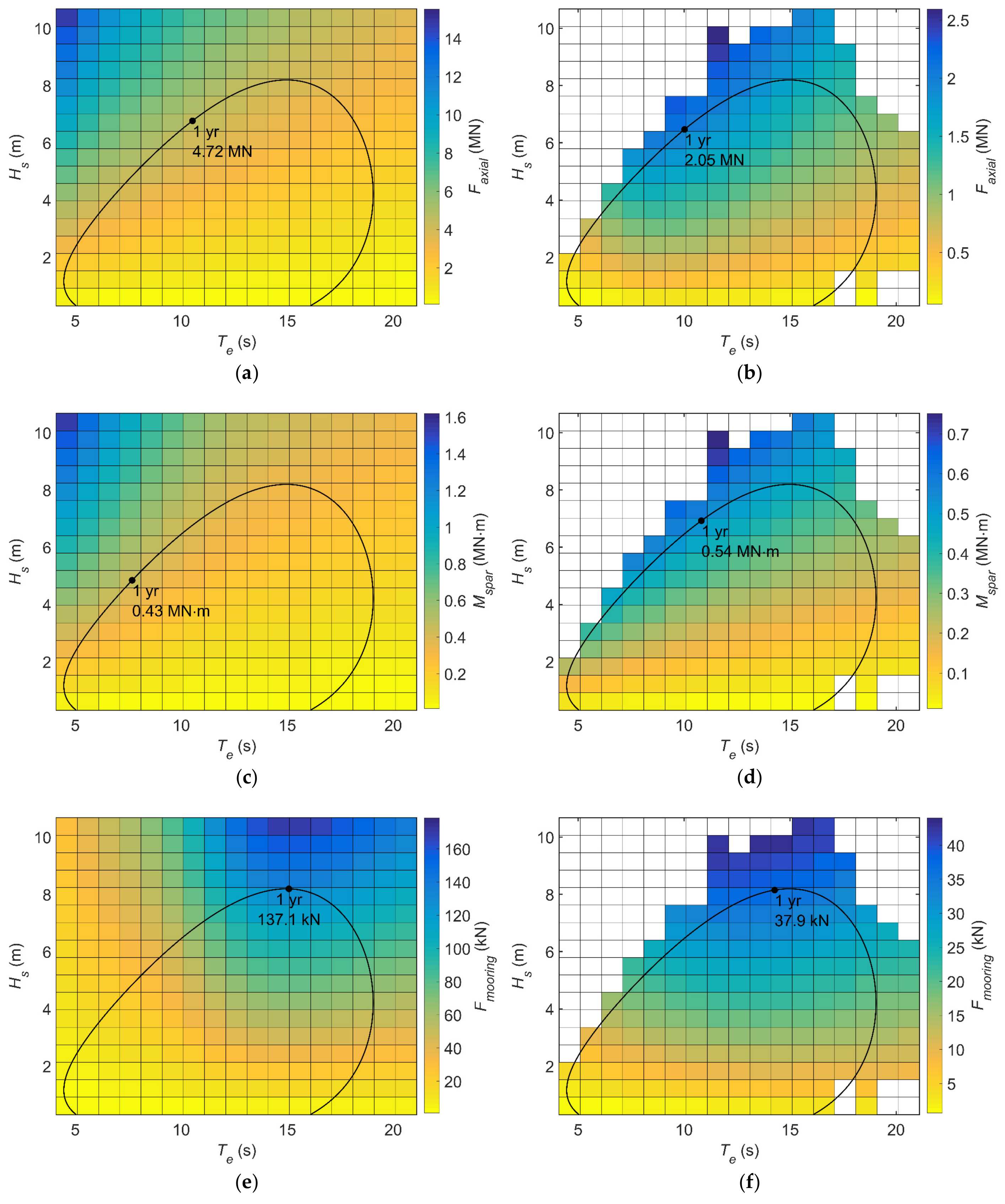
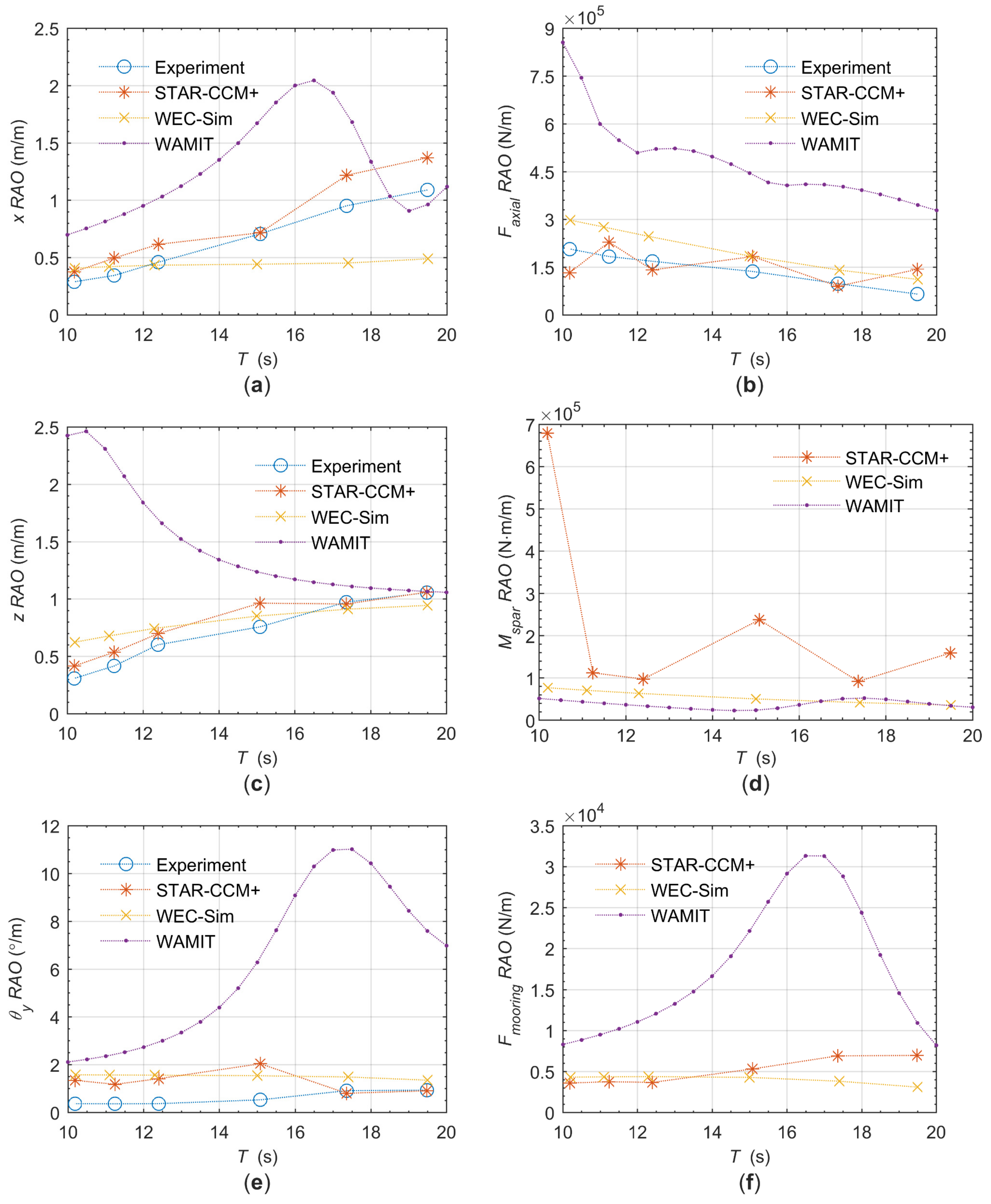
3.1. WAMIT and WEC-Sim Simulation Results

The WAMIT- and WEC-Sim-derived 3-h extreme loads for F_axial, M_spar, and F_mooring for the joint probability distribution given in Figure 2 are plotted in Figure 9. The maximum 3-h extreme loads within the 1-year return period, and the sea states at which they occur, are identified on each of the plots. In each case, the maximum extreme load occurs on the 1-year contour, indicating that for the RM3 WEC, the operational sea states do not dictate the design loads (without considering fatigue loads). Comparing the WAMIT and WEC-Sim results provided in Figure 9, it may be concluded that the WAMIT models provide order-of-magnitude accurate results and successfully identify the approximate sea states at which the most extreme loads occur. However, it is also evident that, despite including linear representations of the viscous drag and mooring stiffness in the WAMIT RAO model, WAMIT cannot accurately capture the nonlinear responses induced by the extreme waves and the experimental model’s mooring system.

The all-sea-state, 1-year long-term design loads for F_axial, M_spar, and F_mooring are provided in Figure 10 for the WAMIT- and WEC-Sim-based results. The point on the plot where the complementary cumulative distribution function crosses the 1-year long-term probability level ($Q=1/N$, where $N=1·365·24·60·60/T$) is the all-sea-state 1-year design load. The 1-year probability level, indicated by the horizontal dashed line, was calculated using the mean wave period in the WAMIT calculations. Technically, the mean response period should be used, as it is in the WEC-Sim calculations. For linear wave-induced motions, this usually results in a negligible difference in the 1-year probability level, as shown in the F_axial results in Figure 10a; however, results in more significant differences between the WAMIT and WEC-Sim M_spar and F_mooring 1-year probability levels, as shown in Figure 10b,c. Because the complementary cumulative distribution function is a probability weighted sum of the short-term extreme loads, the same modeling differences discussed for the 3-h extreme loads are also evident in the 1-year all-sea-state loads. Specifically, WAMIT- and WEC-Sim-derived 1-year all-sea-state design loads are generally of the same order of magnitude; however, a time-domain numerical model (e.g., WEC-Sim) is required to capture the nonlinear responses induced by extreme waves and the 1:100-scale RM3 mooring configuration.

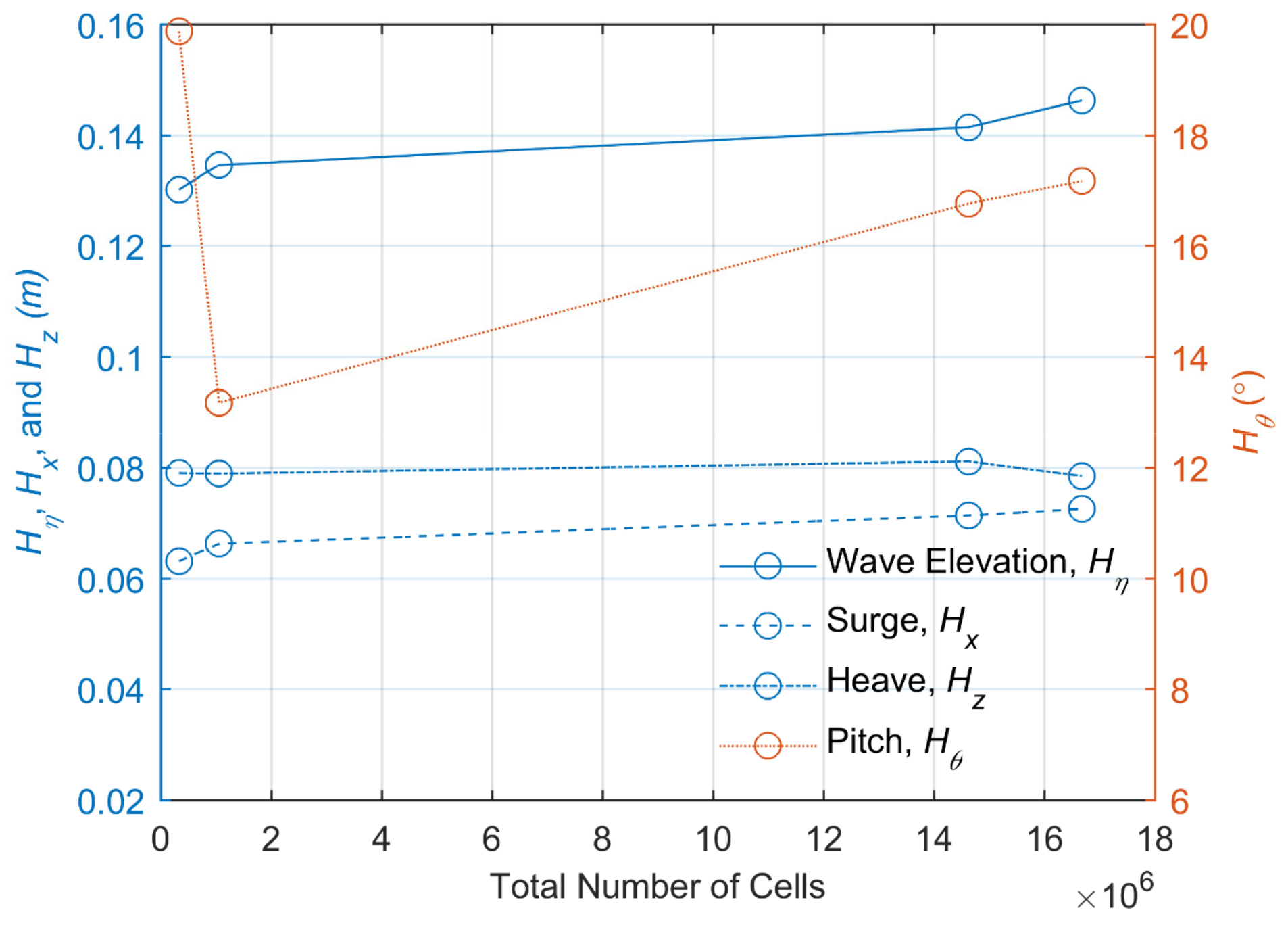
3.2. STAR-CCM+ Regular Wave Simulation Results

The STAR-CCM+ regular wave surge, heave, pitch, F_axial, M_spar, and F_mooring 1:1-scale RAO results are given in Figure 11 and Table 5, where they are compared with experimental, WEC-Sim, and WAMIT RAO results. The average absolute RAO errors for each of the computational models, in comparison to the experimentally measured RAOs, are reported in Table 5. As presented in Figure 11 and Table 5, the STAR-CCM+ results agree reasonably well with the experimental results for surge, heave, pitch, and F_axial. There are no experimental data for M_spar and F_mooring, so for these loads, WEC-Sim and WAMIT errors are relative to the STAR-CCM+ values. The STAR-CCM+ RAO errors, relative to the experimental values, are generally less than the WEC-Sim RAO errors; and the WEC-Sim RAO errors are less than the WAMIT RAO errors, as may be expected based on the model fidelities.

The M_spar RAO response predicted by STAR-CCM+ is significantly larger than the WEC-Sim- or WAMIT-predicted RAO responses. Given the accuracy of the other RANS-FEA results, it is assumed that the STAR-CCM+ M_spar RAO responses are also more accurate. The large difference between the STAR-CCM+ and linear-based M_spar RAO results is likely because the simplified beam model used to calculate the generalized mode displacements, shown in Figure 3b, along with only one mode shape of each type, cannot capture the stress responses and bending moments of the actual three-dimensional structure. Any future structural load studies involving the RM3 geometry should include FEA-derived mode shapes as well as multiple mode shapes of each type, as considered in [9,12].

All the WAMIT-predicted RAO responses differ significantly from the experimental, STAR-CCM+, and WEC-Sim-predicted RAOs. The WAMIT RAO calculations include effects of the mooring system, as an additional linear stiffness term, and viscous damping, as an additional equivalent linear damping term; however, the frequency-domain WAMIT model is unable to capture the nonlinear time-domain responses induced by extreme waves and the two-layered mooring configuration. Although the WAMIT-derived RAOs are generally of the same order of magnitude as those derived from WEC-Sim and STAR-CCM+, the results presented in Figure 11 and Table 5 give an indication of the level of error that might be expected when using a BEM-based loads analysis.

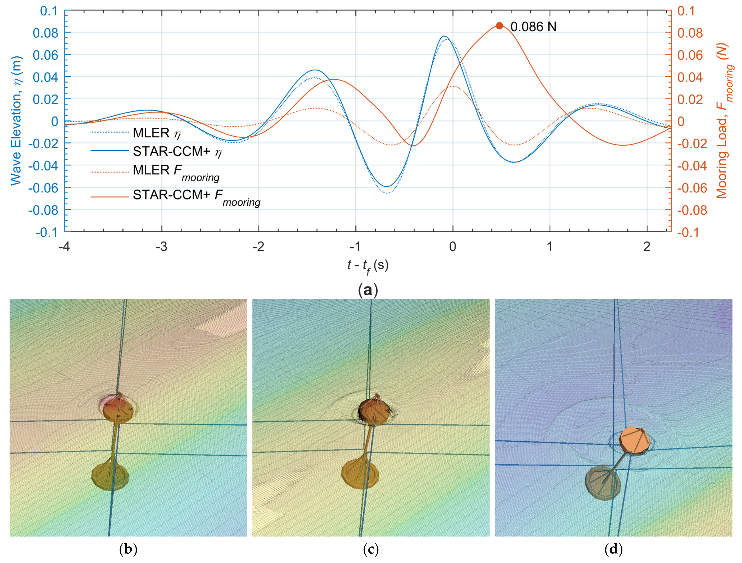
3.3. STAR-CCM+ Most-Likely Extreme Response-Focused Wave Simulation Results

The MLER wave elevations, η (both theoretical and predicted by STAR-CCM+), and F_axial, M_spar, and F_mooring responses are plotted and compared in Figure 12, Figure 13 and Figure 14. As plotted in Figure 12a, Figure 13a, and Figure 14a, there is excellent agreement between the theoretical and simulated wave elevations: The root-mean-square error over the timeframe plotted, between the theoretical and STAR-CCM+ wave elevation, is 0.0035, 0.0015, and 0.0030 m for the F_axial, M_spar, and F_mooring conditioned MLER-focused waves, respectively. However, from the load responses plotted in Figure 12a, Figure 13a, and Figure 14a, it is evident that using the MLER-focused wave approach to estimate the design loads for the RM3 WEC, and its particular mooring configuration, is not effective.

The F_axial MLER-focused wave simulation results are given in Figure 12. In this simulation, from t − t_f ≈ −0.7 to −0.2 s, the focus wave overtops the WEC, as shown in Figure 12b, and from t − t_f ≈ −0.2 to 0.25 s, the float and mooring system rise above the water surface, as shown in Figure 12c. With the float out of the water, there are minimal hydrodynamic forces on the float, and the mooring response produces a large pitch displacement, approximately 35° at t − t_f ≈ 0.29 s, as shown in Figure 12d. With the float first being submerged and then out of the water at the focus time (t − t_f ≈ 0.0 s), the peak F_axial load response predicted by MLER theory is missed entirely.

The M_spar MLER-focused wave simulation results are presented in Figure 13. In this simulation, from t − t_f ≈ −0.8 to −0.2 s the float is slightly above the water surface; from t − t_f ≈ −0.2 to 0.3 s, the float is submerged by the focus wave, as shown in Figure 13b; from t − t_f ≈ 0.3 to 0.9 s, the float and mooring lines are above the water surface, as shown in Figure 13c; from t − t_f ≈ 0.9 to 1.3 s, the float is submerged again, as shown in Figure 13d; and from t − t_f ≈ 1.3 to 1.8 s, the float is slightly above the water surface again. The steep drops in M_spar, around t − t_f ≈ −0.5, 0.7, and 1.9 s, occur as the float emerges from the water surface, reducing the hydrodynamic forces on the float. The large increases in M_spar, around t − t_f ≈ 0.0 and 1.2 s, occur as the float is overtopped and submerged, adding to the hydrodynamic forces and moment on the float. Again, all of these interactions are strongly nonlinear, with minimal correspondence to the linear M_spar responses predicted by the MLER method.

The F_mooring MLER-focused wave simulation results were plotted, without the pretension force, and are visually presented in Figure 14. As with the previous MLER-focused wave simulations, the float is overtopped, from t − t_f ≈ −0.7 to 0.0 s, as shown in Figure 14b, and partially emerges from the water surface, from t − t_f ≈ 0.0 to 1.5 s, as shown in Figure 14c,d. The RANS-FEA simulation predicts an overall larger F_mooring response, with a phase shift, in comparison to the linear MLER theoretical response. These differences are a result of the combined effects of the large surge (and corresponding drift force), heave, and pitch displacements. The maximum surge displacement is 0.09 m, at t − t_f ≈ 0.36 s; the maximum heave displacement is 0.08 m at t − t_f ≈ 0.09 s; and, the maximum pitch displacement is 35° at t − t_f ≈ 0.75 s, all of which may not be considered small, relative to the RM3 geometry, as required by linear theory.

The MLER design wave approach is predicated on the assumption that the nonlinear response can be approximated by a linearized response, and the nonlinear response is a small perturbation of the linear solution. Focused wave approaches have been successfully used in previous studies to evaluate design loads, where the hydrodynamic bodies and wave parameters do not result in interactions that are highly nonlinear [6,25,26,28]. However, in this study, the STAR-CCM+ simulations show highly nonlinear interactions in response to the applied MLER waves, including overtopping and complete submersion, the float and mooring lines rising fully out of the water, large rigid body motions, vortex shedding, flow separation, turbulence, and a strong coupling between the nonlinear hydrodynamic loading, mooring forces, and pitch motions; all of which the linear MLER approach cannot predict.

4. Discussion and Conclusions

The structural design requirements for WEC survival are a key component of WEC development costs, and consequently, the cost of wave energy. Although WEC design practices are evolving, current computational limitations challenge the implementation of these practices and the accurate evaluation of WEC design loads. This case study demonstrates one possible computational framework for evaluating the design loads of a WEC. The framework considered utilizes established design guidelines, where they exist, and follows a progression from many low-fidelity design load estimates to a few high-fidelity design load simulations. The objective of the design load evaluation framework used is to provide a computationally efficient means of accurately calculating a WEC’s structural design loads and the conditions under which these loads occur, within the limitations of today’s computational abilities.

The WEC considered in this case study was the 1:100-scale RM3 model and the loads evaluated were the spar axial force, spar bending moment, and mooring line force. Three design stages were used, wherein the results of the first two stages were used as a basis for the subsequent, higher-fidelity modeling stages, thereby reducing the number of evaluations necessary in the final, more computationally intensive design stage. The first set of design load estimates were made using the BEM code WAMIT. The second set of design load estimates were obtained using a modified version of the linear time-domain code WEC-Sim. The final set of design load calculations were obtained using CFD coupled with FEA to simulate the WEC responses to both regular waves and focused waves. Each of these models were compared and validated with previously obtained regular wave experimental data.

The 1-year design load results for each combination of design load method, sea-state realization method, and modeling method, as applied in this study, are summarized in

Table 6. Comparison of RM3 1:1-scale 1-year design loads as calculated by the various methods.

Design Load Method	Sea-State Realization Method	Modeling Method	Faxial (MN)	Mspar (MN·m)	Fmooring (kN)
One-dimensional	Regular waves	WAMIT	12.15	0.79	445.7
		WEC-Sim	4.44	1.15	67.1
		STAR-CCM+	3.34	9.48	102.4
		Experiment	3.09	-	-
Contour *	Irregular waves	WAMIT	4.72	0.43	137.1
		WEC-Sim	2.05	0.54	37.9
Long term All-sea-state	Irregular waves	WAMIT	5.55	0.49	161.2
		WEC-Sim	2.72	0.82	50.0
Contour *	MLER wave	STAR-CCM+	0.64	0.59	85.7

* Sea states are based on the maximum all-sea-state 3-h extreme loads within the 1-year return contour. As all 3-h extreme loads are on the 1-year return contour; this is effectively the contour design load method.

. Considering the results given in Table 6, the design load evaluation framework utilized in this study was partially successful in assessing the RM3 design loads. Although it is known that linear-based models cannot accurately predict loads for extreme, nonlinear conditions, it was assumed in the use of this framework that linear-based models could predict the approximate sea-state conditions at which the maximum loads are likely to occur, such that higher-fidelity models could be efficiently used at these sea states of interest. Results from the WAMIT, WEC-Sim, STAR-CCM+, and the experimental tests suggest that the linear-based models can roughly approximate the design loads and the sea states at which they occur. However, in this study, the WAMIT-level results did not accurately capture the nonlinear mooring induced responses; the simplified mode shapes used for bending in the linear-based generalized mode method underestimated the three-dimensional structure’s moments; and, the fluid structure interactions for the RM3 model resulted in responses that were too nonlinear to be effectively predicted using the linear-based MLER-focused wave method. There is, however, good agreement in the regular wave RANS-FEA and experimental responses, indicating that the STAR-CCM+ RANS-FEA models are configured correctly and are capable of accurately modeling the nonlinear steady-state responses. Given these considerations, the best estimate of 1-year design loads for the 1:1-scale RM3 WEC, as given in Table 6, is thought to be the one-dimensional, regular wave, STAR-CCM+ values.

In review of the results obtained in this WEC design load case study, several general conclusions and suggestions for future research may be drawn.

• This case study demonstrates one possible design load evaluation framework. However, the evaluation of WEC design loads is still a subject of research, and there are many other possible frameworks and methods for analysis. Even so, with current computational limitations, it will generally be necessary with any analysis framework to follow a progression from low-fidelity modeling methods to high-fidelity modeling methods, as done in this study, to efficiently use high-fidelity simulations and accurately calculate the design loads.
• For WEC configurations in which responses are mostly linear, the design load evaluation framework used in this study will suffice, as shown in previous studies [6,28]. However, based on the results of this study, when using the generalized body modes method, for anything but the simplest geometries, multiple mode shapes of each type and/or FEA-derived mode shapes should be used to obtain accurate structural load estimates using low- and mid-fidelity modeling methods.
• For WEC configurations in which the responses are only slightly nonlinear, the design load evaluation framework demonstrated here should still be sufficient, but with an additional design load evaluation stage in which weakly nonlinear restoring and Froude–Krylov forcing terms are included in WEC-Sim, or similar, models [2,25]. It might be an interesting future study to reconsider the design load evaluation framework demonstrated in this study with the inclusion of this step.
• In this case study, regular waves were more effective in estimating the design loads than focused waves. With this in mind, it may be beneficial in future studies to estimate the nonlinearities of the system (using the low- and mid-fidelity modeling results) prior to conducting focused wave simulations. If the wave structure interactions are expected to be highly nonlinear, high-fidelity regular wave, or even irregular wave, simulations may be more informative.
• Recently, computational advances have made 3-h irregular wave CFD simulations possible, as reported in [29]. With this as an option, a very informative potential future study could be to compare the accuracy of equivalent regular and focused wave load results, for a given sea state, to 3-h irregular wave load results.
• For WEC configurations in which the wave structure interactions and responses are highly nonlinear, new computationally efficient, high-fidelity simulation methods must be developed to accurately evaluate WEC design loads and the conditions under which they occur. In the near term, this could potentially include the development of linear-RANS hybrid models. In the long term, it is possible that computational capabilities may be advanced enough that the all-sea-state, long-term irregular wave, RANS-FEA simulations can be run directly.

References

1. Coe, R.; Yu, Y.-H.; van Rij, J. A Survey of WEC Reliability, Survival and Design Practices. Energies 2017, 11, 4. [Google Scholar] [CrossRef]
2. Van Rij, J.; Yu, Y.-H.; Coe, R.G. Design Load Analysis for Wave Energy Converters. In Proceedings of the 37th International Conference on Ocean, Offshore & Arctic Engineering (OMAE2018), Madrid, Spain, 17–22 June 2018. [Google Scholar]
3. International Electrotechnical Commission. Marine Energy—Wave, Tidal and Other Water Current Converters—Part 2: Design Requirements for Marine Energy Systems; IEC: Geneva, Switzerland, 2016. [Google Scholar]
4. NORSOK. Actions and Action Effects; Standards Norway: Oslo, Norway, 2007. [Google Scholar]
5. Det Norske Veritas. Recommended Practice: Environmental Conditions and Environmental Loads; DNV: Oslo, Norway, 2007. [Google Scholar]
6. Quon, E.; Platt, A.; Yu, Y.-H.; Lawson, M. Application of the Most Likely Extreme Response Method for Wave Energy Converters. In Proceedings of the 35th International Conference on Ocean, Offshore and Arctic Engineering (OMAE2016), Busan, Korea, 19–24 June 2016. [Google Scholar]
7. Lee, C.; Newman, J. WAMIT® User Manual Version 7.1; WAMIT, Inc.: Chestnut Hill, MA, USA, 2015. [Google Scholar]
8. NEMOH. Available online: https://lheea.ec-nantes.fr/logiciels-et-brevets/nemoh-presentation-192863.kjsp?RH=1489593406974 (accessed on 29 July 2019).
9. Van Rij, J.; Yu, Y.-H.; Guo, Y. Structural Loads Analysis for Wave Energy Converters. In Proceedings of the 36th International Conference on Ocean, Offshore & Arctic Engineering (OMAE2017), Trondheim, Norway, 25–30 June 2017. [Google Scholar]
10. Newman, J.N. Wave effects on deformable bodies. Appl. Ocean Res. 1994, 16, 47–59. [Google Scholar] [CrossRef]
11. WEC-Sim. Available online: https://wec-sim.github.io/WEC-Sim/ (accessed on 29 July 2019).
12. Guo, Y.; Yu, Y.-H.; van Rij, J.; Tom, N. Inclusion of Structural Flexibility in Design Load Analysis for Wave Energy Converters. In Proceedings of the European Wave and Tidal Energy Conference, Cork, Ireland, 27 August–1 September 2017. [Google Scholar]
13. Yu, Y.-H.; Lawson, M.; Li, Y.; Previsic, M.; Epler, J.; Lou, J. Experimental Wave Tank Test for Reference Model 3 Floating-Point Absorber Wave Energy Converter Project; National Renewable Energy Laboratory: Golden, CO, USA, 2015. [Google Scholar]
14. Reference Model Project. Available online: https://energy.sandia.gov/energy/renewable-energy/water-power/technology-development/reference-model-project-rmp/ (accessed on 29 July 2019).
15. Coe, R.; Michelen, C.; Eckert-Gallup, A.; Yu, Y.-H.; van Rij, J. WDRT: A Toolbox for design-response analysis of wave energy converters. In Proceedings of the Proceedings of the 4th Marine Energy Technology Symposium (METS2016), Washington, DC, USA, 25–27 April 2016. [Google Scholar]
16. Coe, R.; Michelen, C.; Eckert-Gallup, A.; Martin, N.; van Rij, J.; Yu, Y.-H.; Quon, E.; Manuel, L.; Nguyen, P.; Canning, J.; et al. WEC Design Response Toolbox (WDRT). Available online: https://wec-sim.github.io/WDRT/ (accessed on 29 July 2019).
17. Kert-Gallup, A.C.; Sallaberry, C.J.; Dallman, A.R.; Neary, V.S. Application of principal component analysis (PCA) and improved joint probability distributions to the inverse first-order reliability method (I-FORM) for predicting extreme sea states. Ocean Eng. 2016, 112, 307–319. [Google Scholar] [CrossRef] [Green Version]
18. Kelly, S.G. Theory and Problems of Mechanical Vibrations; McGraw-Hill: New York, NY, USA, 1993. [Google Scholar]
19. Faltinsen, O.M. Sea Loads on Ships and Offshore Structures; Cambridge University Press: Cambridge, UK, 1993. [Google Scholar]
20. Cummins, W.E. The Impulse Response Function and Ship Motions; Department of the Navy, David Taylor Model Basin: Bethesda, MD, USA, 1962. [Google Scholar]
21. Hall, M. MoorDyn User’s Guide; Department of Mechanical Engineering, University of Maine: Orono, ME, USA, 2015. [Google Scholar]
22. Michelen, C.; Coe, R. Comparison of Methods for Estimating Short-Term Extreme Response of Wave Energy Converters. In Proceedings of the IEEE Oceans 2015, Washington, DC, USA, 19–22 October 2015. [Google Scholar]
23. Coe, R.G.; Michelen, C.; Eckert-Gallup, A.; Sallaberry, C. Full long-term design response analysis of a wave energy converter. Renew. Energy 2018, 116, 356–366. [Google Scholar] [CrossRef]
24. STAR-CCM+ | MDX. Available online: https://mdx.plm.automation.siemens.com/star-ccm-plus (accessed on 29 July 2019).
25. Van Rij, J.; Yu, Y.-H.; Tom, N. Validation of Simulated Wave Energy Converter Responses to Focused Waves for CCP-WSI Blind Test Series 2. In Proceedings of the 13th European Wave and Tidal Energy Conference Series (EWTEC), Napoli, Italy, 1–6 September 2019. [Google Scholar]
26. Ransley, E.J.; Greaves, D.; Raby, A.; Simmonds, D.; Hann, M. Survivability of wave energy converters using CFD. Renew. Energy 2017, 109, 235–247. [Google Scholar] [CrossRef] [Green Version]
27. Yu, Y.-H.; Li, Y. Reynolds-Averaged Navier–Stokes simulation of the heave performance of a two-body floating-point absorber wave energy system. Comput. Fluids 2013, 73, 104–114. [Google Scholar] [CrossRef]
28. Coe, R.G.; Rosenberg, B.J.; Quon, E.W.; Chartrand, C.C.; Yu, Y.-H.; van Rij, J.; Mundon, T.R. CFD design-load analysis of a two-body wave energy converter. J. Ocean Eng. Mar. Energy 2019, 5, 1–19. [Google Scholar] [CrossRef]
29. Baquet, A.; Jang, H.; Lim, H.-J.; Kyoung, J.; Tcherniguin, N.; Lefebvre, T.; Kim, J. CFD-Based Numerical Wave Basin for FPSO in Irregular Waves. In Proceedings of the ASME 2019 38th International Conference on Ocean, Offshore and Arctic Engineering, Glasgow, UK, 9–14 June 2019. [Google Scholar]
Figure 1. RM3 1:100-scale model [13].
Jmse 07 00250 g001
Figure 2. Joint probability distribution for the National Data Buoy Center (NDBC) Buoy 46022 and RM3 tank test data (HsH/1.9, Te ≈ 1.206 T).
Jmse 07 00250 g002
Figure 3. RM3 WAMIT model: (a) BEM panel representation; (b) generalized body-mode representation; (c) normalized axial displacement mode, mass, and stiffness; (d) normalized bending displacement mode, mass, and stiffness.
Jmse 07 00250 g003
Figure 4. RM3 WEC-Sim model.
Jmse 07 00250 g004
Figure 5. 1:100-scale STAR-CCM+ CFD domain and grid refinement zones for test number 17, t = 20.37 s.
Jmse 07 00250 g005
Figure 6. Grid convergence for test number 16.
Jmse 07 00250 g006
Figure 7. 1:100-scale STAR-CCM+ FEA simulation for test number 17, t = 20.37 s.
Jmse 07 00250 g007
Figure 8. 1:100-scale RM3 MLER-focused wave inputs: (a) Faxial RAO; (b) Faxial S(Hs = 0.065, Tp = 1.169); (c) Mspar RAO; (d) Mspar S(Hs = 0.069, Tp = 1.262); (e) Fmooring RAO; (f) Fmooring S(Hs = 0.081, Tp = 1.664).
Jmse 07 00250 g008aJmse 07 00250 g008b
Figure 9. Three-hour extreme loads: (a) WAMIT-calculated Faxial; (b) WEC-Sim-calculated Faxial; (c) WAMIT-calculated Mspar; (d) WEC-Sim-calculated Mspar; (e) WAMIT-calculated Fmooring; (f) WEC-Sim-calculated Fmooring.
Jmse 07 00250 g009
Figure 10. WAMIT- and WEC-Sim-calculated 1-year, long-term, all-sea-state extreme loads: (a) Faxial; (b) Mspar; (c) Fmooring.
Jmse 07 00250 g010
Figure 11. Simulated versus experimentally measured RAOs: (a) x, surge; (b) Faxial, axial force; (c) z, heave; (d) Mspar, bending moment; (e) θy, pitch; (f) Fmooring, mooring force.
Jmse 07 00250 g011
Figure 12. 1:100-scale RM3 MLER-focused wave results for the spar axial force: (a) ƞ(ttf) and Faxial(ttf), (b) Response at ttf = −0.375 s, (c) Response at ttf = 0.043 s, and (d) Response at ttf = 0.294 s.
Jmse 07 00250 g012
Figure 13. 1:100-scale RM3 MLER-focused wave results for the spar bending moment: (a) ƞ(ttf) and Mspar(ttf), (b) response at ttf = 0.089 s, (c) response at ttf = 0.732 s, and (d) response at ttf = 1.145 s.
Jmse 07 00250 g013
Figure 14. 1:100-scale RM3 MLER-focused wave results for the mooring line force: (a) ƞ(ttf) and Fmooring(ttf), (b) response at ttf = −0.159 s, (c) response at ttf = 0.017 s, and (d) response at ttf = 0.486 s.
Jmse 07 00250 g014