Numerical and Experimental Modelling of a Wave Energy Converter Pitching in Close Proximity to a Fixed Structure

Abstract

Free-floating bodies are commonly modelled using Cummins’ equation based on linear potential flow theory and including non-linear forces when necessary. In this paper, this methodology is applied to a body pitching around a fixed hinge (not free-floating) located close to a second bottom-fixed body. Due to the configuration of the setup, strong hydrodynamic interactions occur between the two bodies. An investigation is made into which non-linear forces need to be included in the model in order to accurately represent reality without losing computational efficiency. The non-linear forces investigated include hydrostatic restoring stiffness and different formulations of excitation forces and quadratic drag forces. Based on a numerical comparison, it is concluded that the different non-linear forces, except for the quadratic drag force, have a minor influence on the calculated motion of the pitching body. Two formulations of the quadratic drag force are shown to result in similar motions, hence the most efficient one is preferred. Comparisons to wave basin experiments show that this model is, to a large extent, representative of reality. At the wave periods where the hydrodynamic interactions between the bodies are largest, however, the amplitudes of motion measured in the wave basin are lower than those calculated numerically.

1. Introduction

Wave energy converter (WEC) developers need to prove the economic viability of their concepts and need to get funding to complete the technology development. So, despite the large number of wave energy concepts, only a few are grid-connected commercialized in the world. Wave energy devices have to be economically viable, which depends on their performance. The techno-economical assessment is as important as the evaluation of the technology readiness [1].

The principle of wave energy conversion is based on the ability for a body to absorb the incoming wave energy, which depends straightforwardly on its hydrodynamic design. According to Reference [2], symmetric bodies, such as heaving point absorbers and pitching flaps, have a theoretical limit in wave energy absorption of 50%. However, for a non-symmetric bodies, such as Salter’s duck concept (invented and developed since 1974 [3]), the absorption ratio can be close to 100%.

Salter’s duck is, according to the categorization defined in Reference [4], a non-symmetric rotating floating wave activated body. Floating Power Plant’s WEC [5], the case-study in this paper, is also a non-symmetric rotating floating wave activated body but it is part of a hybrid concept that combines wind power and wave energy conversion (see Figure 1, left). Floating Power Plant (hereafter FPP) is a close-to-market technology that has been under development since 1995. The pioneering technology was the P37 device, Poseidon, which was a 1:25-scale prototype tested offshore in Denmark during four different periods from 2008 until 2013. The P37 was the first device in the world to provide electricity to the grid from wind and wave resources simultaneously.

The FPP device is the result of several years of research, wave flume, wave basin and offshore testing [6,7]. The FPP full-scale device is a floating foundation for a wind turbine in which four WECs are integrated into the semisubmersible platform. The device is designed so that each pitching WEC (patented) interacts with the supporting semisubmersible structure, amplifying its motion within the design wave frequency range. In the original design (1995), each WEC rotated about the horizontal plane but at this early stage they had a very simplistic wedge-like geometry, and their interaction with the substructure was limited to the axis about which they rotated. As hydrodynamic multi-body models were very limited at the time, the development process was largely dominated by physical testing of variations of the design. Since then, the design has been modified and optimized according to the experience and knowledge gathered through the years of research.

The objective of numerical models for WECs is to simulate hydrodynamic loads and body motions under different sea conditions. For hybrid or multi-body devices that co-locate different systems on the same structure, the objective is twofold: to simulate loads and motions and to understand the interactions that may occur between the different components that make up the technology.

There is no software that has proven valid for all or the majority of the problems that modelling WECs presents. Wave energy developers use different software packages or codes to simulate the performance of WECs in operational and extreme conditions. In addition, there is a very limited amount of experimental data that has been published and is high enough quality for code validation. However, some research groups, like OES Task 10 [8], are working towards the goal of building confidence in numerical estimations of loads and power production [9]. There are three categories to group the variety of approaches to simulating WECs: linear codes, quasi-linear codes and non-linear codes [10]. Linear codes are based on linear potential flow theory, computationally inexpensive and numerically stable, over-simplistic in many cases. Quasi-linear codes (or weakly non-linear codes) are based on linear theory but include some non-linear effects. These non-linear effects commonly include some or all of instantaneous hydrodynamic forces, quadratic drag loads or the non-linear power-take-of forces [11,12,13]. Finally, codes that account for strong non-linearities include both fully non-linear time domain boundary element models and computational fluid dynamics models (CFD). Although the accuracy is highest for fully non-linear codes, quasi-linear codes may be preferable due to the reduction in computational time.

There exist some software packages for wave energy converters, such as the open-source WEC-Sim [14] or the commercial code WaveDyn, developed by DNV-GL. One of the challenges they face, and that is addressed in this paper, is the interaction between moving bodies that are closely located. Particularly, pitch motion is the degree of freedom that shows the biggest discrepancies between codes according to a WEC code comparison project [15]. Further to this, limitations to WEC-Sim have been reported when trying to validate the numerical model of pitching closely spaced bodies by comparison to physical test data [16].

The numerical model presented in this paper solves Newton’s second law with a quasi-linear approach. Varying levels of non-linearity are included and compared. By comparison to experimental data, the authors suggest a model based on a compromise between accuracy and computational effort. Floating Power Plant is the case study. Hence, the aim of this paper is twofold. First, to establish a numerical model based on radiation-diffraction solver to calculate hydrodynamics and motions of the pitching body. And secondly, to use the model to evaluate the influence of the multi-body interactions on the dynamic response of the pitching body. The physical data used to validate the numerical model in this paper is based on a simplified representation of the FPP device. In the simplified setup, a single WEC and a fixed structure located in close proximity are considered, see Figure 1. Large interaction effects between the WEC and fixed structure are seen in the experimental data, although the motion of the platform and possible interactions between neighbouring WECs are excluded.

2. Research Question

This paper compares linear and non-linear formulations of hydrodynamic and hydrostatic moments acting on a pitching hinged device in close proximity to a bottom-mounted substructure. Linear theory predicts strong interactions between the two bodies due to the setup, and these interactions were also observed during wave basin experiments. The objective of the study is to conclude on a numerical model that provides a good balance between accuracy and computational cost based on comparison with experimental data. The experimental data comes from wave basin experiments planned to provide high-quality data for numerical model validation. The method used (both experimental and numerical) isolates the different moments acting on the device: hydrostatic moments through slow motion tests, radiation moments through free decay tests and diffraction moments through fixed-device tests. Once the formulation of the numerical model is decided, its suitability for simulating reality is checked with the full problem of a freely-responding pitching body in regular waves.

3. Numerical Model Description

Figure 2 shows the profile of the model of the FPP’s wave energy converter (WEC) used during the experimental campaign. The origin of the body coordinate system is located at the middle of the rotation shaft. The origin of the global coordinate system is located at the still water line directly underneath the origin of the body coordinate system. The pitch angle of rotation, $\theta$, is defined by the inclination of the hinge-arm relative to the horizontal x-axis. The particle motion is calculated referred to the global coordinate system, which has the $z^{\prime }$ coordinate at the still water line.

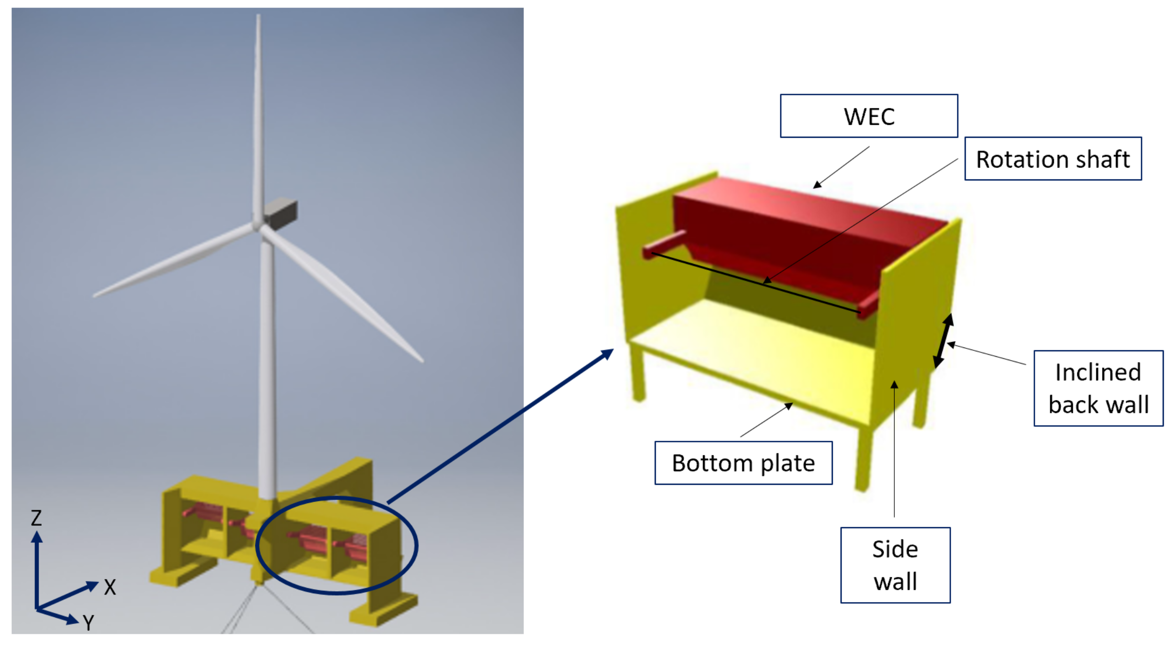
3.1. Geometry Definition

The geometry of the WEC is defined from physical measurements and drawn in MultiSurf using patches defined by B-splines and C-splines, which are continuous smooth surfaces in space. This geometry is analysed by WAMIT using the higher-order method [17]. To implement forces external to WAMIT, the body is discretized into a series of planar panels. The planar panels are initially output from WAMIT as a list of cartesian coordinates of the vertices of quadrilateral panels. Each quadrilateral panel is then subdivided into two triangular panels. Suppose a triangular panel has three vertices $(v_1,v_2,v_3)$ defined by cartesian coordinates [18]. The centroid, unit normal vector and surface area of the triangular planar panel are then defined by

$$\begin{array}{cc}\overrightarrow{x}\hfill & =[x,y,z]=\frac{1}{3}\sum _{i=1}^3{v}_i\hfill \end{array}$$

(1)

$$\begin{array}{cc}\overrightarrow{n}\hfill & =[n_x,n_y,n_z]={\displaystyle \frac{(v_2-v_1)\times (v_1-v_3)}{\sqrt{\parallel v_2-v_1{\parallel }^2\parallel v_1-v_3{\parallel }^2-{\parallel (v_2-v_1)·(v_1-v_3)\parallel }^2}}}\hfill \end{array}$$

(2)

$$\begin{array}{cc}S\hfill & =\frac{1}{2}\parallel (v_2-v_1)\times (v_1-v_3)\parallel ,\hfill \end{array}$$

(3)

where $\parallel \parallel$ is the absolute value and × the cross product [19].

Where body-surface integration is calculated, a discrete integral is performed in which it is assumed that point forces act at the centroid of each triangular panel. The panel centroids and their normal vectors are defined initially for an angle of the body equal to zero according to the body coordinate system given in Figure 2. The following rotation matrix is then used to calculate the new components if the WEC rotates an angle $\theta$ about the origin of the body coordinate system [20]:

$$R_y\left(\theta \right)=\left[\begin{array}{ccc}cos\left(\theta \right)& 0& sin\left(\theta \right)\\ 0& 1& 0\\ -sin\left(\theta \right)& 0& cos\left(\theta \right)\end{array}\right]$$

(4)

With the aim of speeding up the calculations that use panel centroids, only a portion or slice in the y direction of the WEC is used. A width ratio is applied afterwards to scale up the volume and loads to the actual size of the body. Figure 2 presents a top view of half of the WEC in blue, and the slice of the WEC used to make the model more efficient in red. Even though the hinge-arms can get slightly submerged for some rotation angles, neglecting them in this simplification does not significantly change the total submerged volume (the difference is less than 3% when fully submerged) or the geometry that defines the hydrodynamic coefficients. The WEC gets out of the water when it rotates more than 20.5 degrees anticlockwise and gets fully submerged when pitches 19 degrees clockwise.

3.2. Equation of Motion

The equation governing the hydrodynamic response of the WEC is Newton’s second law:

$$J{\ddot{X}}_5=M_{grav}+M_{buoy}+M_{rad}+M_{exc}+M_c+M_{drag}+M_{fb},$$

(5)

where J is the mass moment of inertia in pitch (around the y axis), ${\ddot{X}}_5$ is the angular acceleration of the body in pitch, $M_{grav}$ is the gravitational moment, $M_{buoy}$ is the buoyancy moment, $M_{rad}$ is the radiation damping moment, $M_{exc}$ is the wave excitation moment, $M_c$ is the control moment provided by the power-take-off, $M_{drag}$ is the quadratic drag moment and $M_{fb}$ is the friction moment from the bearings. In this paper, the power-take-off only provides a load to set the initial position of the WEC during decay tests, although it is used to measure the hydrostatic moment during slow-motion tests and the wave excitation loads during fixed-WEC experiments.

The numerical model baseline is a set of data of hydrodynamic coefficients calculated using the commercial fluid-structure interaction software WAMIT. WAMIT uses a boundary element method to determine the hydrodynamic coefficients using linear wave theory. The baseline dataset includes the hydrodynamic coefficients for a range of wave frequencies and for different body positions, which are defined by the angle of inclination of the WEC. Under the assumptions of linear wave theory, the amplitudes of motion are assumed to be small, so that the variation in the submerged geometry is negligible. The hydrodynamic quantities corresponding to the pitch degree of freedom of the WEC at the position $\theta =5$ degrees, which is very close to the hydrostatic equilibrium position, are shown in Figure 3 for different wave periods. As the figure illustrates, strong hydrodynamic interactions occur with the inclusion of the bottom-fixed second body. The only unaffected parameter is the Froude-Krylov moment since it depends only on the undisturbed dynamic pressure over the wetted surface of the WEC. The inclusion of the bottom box close to the pitching WEC spans the natural pitch frequency of the WEC, as linear theory predicts and as it has been observed during experiments. A more detailed analysis of the hydrodynamic coefficients calculated by WAMIT for this WEC is included in Reference [21].

In contrast to the assumptions of linear theory, the amplitude of motion of the FPP’s WEC is not necessarily small. Further to this, the geometry of the WEC is non-uniform, meaning larger amplitudes of motion would result in significant changes in the submerged geometry and water-plane area.

3.3. Model Versions

Different formulations of the moments of the dynamic equation of motion are compared, in which varying levels of non-linearity are considered.

3.3.1. Water Surface Elevation: $\eta$

The complex amplitude for the free surface elevation is given by

$$\widehat{\eta }={\displaystyle \frac{H}{2}}\left(e^{-ik{x}^{\prime }cos\beta -ik{x}^{\prime }sin\beta +\phi }\right),$$

(6)

where H is wave height, $\omega$ is angular frequency; k is the wavenumber, $x^{\prime }$ is coordinate in the wave propagation direction, $\beta$ is the angle between the positive x-axis and the direction of propagation of the incident wave and $\phi$ is a phase shift. The real part of Equation (6) defines the water free surface elevation $\eta$.

A phase of $\phi =0$ results in a cosine wave at $x^{\prime }=0$. For heading cosine waves, $\beta =0$ degrees and Equation (6) simplifies to

$$\eta (x^{\prime },t)=\Re \left(\widehat{\eta }{e}^{i\omega t}\right),$$

(7)

which can be written as

$$\eta (x^{\prime },t)={\displaystyle \frac{H}{2}}cos(-ik{x}^{\prime }+\omega t).$$

(8)

3.3.2. Radiation Moment: $M_{rad}$

The radiation moment has been included as a memory function approximated using Prony’s method in the time domain model [22].

$$M_{rad}=-A_{\infty }\left({\theta }_0\right){\ddot{X}}_5\left(t\right)-{\int }_0^{t}K(t-\tau ){\dot{X}}_5\left(\tau \right)d\tau ,$$

(9)

where $A_{\infty }\left({\theta }_0\right)$ is the infinite frequency added mass for the WEC’s rest position ${\theta }_0$, ${\ddot{X}}_5$ is the pitch acceleration, K is the retardation function, t is time and ${\dot{X}}_5$ the pitch velocity.

The first term, $-A_{\infty }\left({\theta }_0\right){\ddot{X}}_5\left(t\right)$, represents the contribution to the force that is in phase with the body acceleration. The second, ${\int }_0^{t}K(t-\tau ){\dot{X}}_5\left(\tau \right)d\tau$, is the convolution term that accounts for the fluid memory effects. K can be calculated in the time domain from the application of Fourier Transform using the frequency dependent radiation damping coefficients (B) for the rest position of the WEC,

$$K\left(t\right)={\displaystyle \frac{2}{\pi }}{\int }_0^{\infty }B(\omega ,{\theta }_0)cos\left(\omega t\right)d\omega .$$

(10)

3.3.3. Hydrostatic Moment: $M_{hyst}$

In general terms, the linear hydrostatic stiffness moment, $M_{hyst}$, is a linearization of the sum between the buoyancy and gravity moments.

Linear Hydrostatic Moment

Assuming small amplitudes of motion (small changes in waterplane area), the hydrostatic moment is:

$$M_{hyst\left(5\right)}=-{\zeta }_{(5,5)}{X}_5=M_{grav\left(5\right)}\left({\theta }_0\right)+M_{buoy\left(5\right)}\left({\theta }_0\right),$$

(11)

where ${\zeta }_{(5,5)}$ is the $(5,5)$ component of the linear hydrostatic stiffness coefficient matrix, $X_5$ is the body’s displacement in the 5th degree of freedom and $M_{grav\left(5\right)}\left({\theta }_0\right)$ and $M_{buoy\left(5\right)}\left({\theta }_0\right)$ are the gravity and buoyancy torque at the WEC’s rest position.

When the assumption of small amplitudes of motion is no longer valid, the hydrostatic moment can be calculated by computing gravity torque and buoyancy torque separately.

Gravity Moment, $M_{grav}$:

The gravity torque depends on the body position defined by the angle of rotation $\theta$ (Figure 2). The gravity torque can be estimated at the rest position ($\theta ={\theta }_0$), and at the instantaneous body position ($\theta ={\theta }_i$) when using a nonlinear approach.

$$M_{grav\left(5\right)}\left(\theta \right)=m_{(1,1)}gCO{G}_x\left(\theta \right),$$

(12)

where m is the $(1,1)$ is the mass of the WEC and $CO{G}_x$ is the x coordinate of the centre of gravity. The gravity moment is equal to the magnitude of the gravity force, which is a vertical force, multiplied by the perpendicular distance between its line of action and the axis of rotation. Since the gravity force is a vertical force, the moment arm is equal to the horizontal component of the centre of gravity, $CO{G}_x$.

Buoyancy Moment, $M_{buoy}$:

Decomposing the body surface into N number of panels ([23,24]), the force due to the hydrostatic pressure in each panel is calculated as in (13),

$$\overrightarrow{F_j}=[F_{(x^{\prime },j)},F_{(y^{\prime },j)},F_{(z^{\prime },j)}]=P_{stat}S\overrightarrow{n}, \mathrm{where} P_{stat}=-\rho g{z}^{\prime },$$

(13)

where S is the surface area, $\overrightarrow{n}$ is the unit normal vector of panel j and $z^{\prime }$ the vertical coordinate of the panel centroid. The integration of the pressure over the body surface results in a non-zero force in the vertical direction (the horizontal forces cancel on a closed surface). The buoyancy force, an upward vertical force exerted by the fluid opposing the weight of the WEC, is given by $F_{buoy}={\sum }_{j=1}^N{F}_{(z^{\prime },j)}$.

The moment due to the static water pressure in roll, pitch and yaw can be found by:

$${\overrightarrow{M}}_{buoy}=\sum _{j=1}^N\left([x^{\prime },y^{\prime },z^{\prime }]\times [F_{(x^{\prime },j)},F_{(y^{\prime },j)},F_{(z^{\prime },j)}]\right),$$

(14)

where $[x^{\prime },y^{\prime },z^{\prime }]$ are the cartesian coordinates of the jth panel and × represents cross product. In this paper, only the moments in pitch are required, hence Equation (14) reduces to

$$M_{buoy\left(5\right)}=\sum _{j=1}^N\left(z^{\prime }{F}_{(x^{\prime },j)}-x^{\prime }{F}_{(z^{\prime },j)}\right).$$

(15)

The buoyancy torque can be estimated at the rest position ($\theta ={\theta }_0$), and at the instantaneous body position ($\theta ={\theta }_i$) when using a nonlinear approach.

3.3.4. Excitation Moment: $M_{exc}$

Excitation moment is the moment on the body around the hinge due to the incident and scattered waves. It can be defined as the sum of Froude-Krylov and scattering moment, or by convolving the instantaneous water surface elevation with the impulse response function of the linear excitation moment.

Froude-Krylov, $M_{FK}$:

Froude-Krylov forces are based on the formulation of the undisturbed dynamic pressure according to linear theory. Under the assumption of linear wave theory, the undisturbed dynamic pressure due to heading regular waves with angular frequency $\omega$ at a point in the fluid $(x^{\prime },y^{\prime },z^{\prime })$ is given by

$$P_{dyn}^{\left[1\right]}=\rho g{\displaystyle \frac{cosh\left(k\left(z^{\prime }+d\right)\right)}{cosh\left(kd\right)}}\eta (x^{\prime },t),$$

(16)

where $\rho$ is water density; g, gravity acceleration; k, wave number; d, water depth and t is the time, respectively. With the instantaneous water surface elevation $\eta (x^{\prime },\omega ,t)$ as in Equations (6) to (8).

Under the assumptions of linear wave theory, variations in volume due to changes in the water surface elevation are not accounted for. Equation (16) is therefore only valid for $z^{\prime }\le 0$. To include the wave kinematics above the still water line, Wheeler stretching is applied as in Reference [25] to give an alternative formulation for the dynamic pressure,

$$P_{dyn}^{\left[2\right]}=\rho g{\displaystyle \frac{cosh\left(k\left({\displaystyle \frac{z^{\prime }-\eta }{1+\frac{\eta }{d}}}+d\right)\right)}{cosh\left(kd\right)}}\eta (x^{\prime },\omega ,t),$$

(17)

where $\eta$ is the water surface elevation $\eta (x^{\prime },\omega ,t)$ as in Equations (6) to (8). Then, using a similar process as the calculation of the buoyancy moment in pitch (Equations (13) to (15)), the Froude-Krylov moment in pitch is given by

$$M_{FK\left(5\right)}=\sum _{j=1}^N\left(z^{\prime }{P}_{dyn}S{n}_x-x^{\prime }{P}_{dyn}S{n}_z\right).$$

(18)

where S is the surface area and $(n_x,n_y,n_z)$ is the unit normal vector of panel j.

The different versions of the numerical model calculate Equation (18) with $P_{dyn}$ calculated as either $P_{dyn}^{\left[1\right]}$ (Equation (16) ) or $P_{dyn}^{\left[2\right]}$ (Equation (17)). Where $P_{dyn}=P_{dyn}^{\left[1\right]}$, the submerged body geometry is calculated either at the rest position (${\theta }_0$) or at the instantaneous position (${\theta }_i$). Where $P_{dyn}=P_{dyn}^{\left[2\right]}$, the submerged body geometry is calculated at the instantaneous position (${\theta }_i$).

Scattering Moment:, $M_{sc}$:

Using WAMIT output values for the scattered moment amplitude ($\parallel M_{sc\left(5\right)}\parallel$) and phase (${\phi }_{sc\left(5\right)}$), the equation of the scattered moment in pitch can be written as

$$M_{sc\left(5\right)}=\Re (\parallel M_{sc\left(5\right)}\parallel e^{i{\phi }_{sc\left(5\right)}}\widehat{\eta }{e}^{i\omega t}),$$

(19)

where $\widehat{\eta }$ is the complex amplitude of the water surface elevation as in Equation (6).

For a nonlinear approach, the WAMIT baseline dataset is interpolated to approximate the scattered moment for the instantaneous body position. The WAMIT dataset consists of data for angles of inclination between −9 and 17 degrees, with an angle increment of 0.2 degrees (data for 127 different angles). The WAMIT values of the scattered moment are computed for a steady state system. Dynamically passing through an angle is clearly not the same as reaching steady state oscillating about that angle. However, this approach accounts for changes in submerged geometry, allowing the scattered moment to be dependent on the submerged body geometry, as Froude-Krylov is. This is particularly important to ensure that the scattering moment tends to zero as the submerged volume tends to zero.

Implementation of Measured Water Surface Elevation

As opposed to assuming a simple cosine wave, it can be advantageous to directly input the measured waves from physical tests. To do this, the excitation moment is calculated by performing the convolution of the impulse response function of the linear theoretical excitation moment ($M_{exc}^{IRF}$) with the measured water surface elevation ( ${\eta }_{EXP}$). The time varying excitation moment is given by Reference [26],

$$M_{exc}\left(t\right)=M_{exc}^{IRF}\left(t\right){\eta }_{EXP}\left(t\right)={\int }_{-\infty }^{\infty }{M}_{exc}^{IRF}(t-\tau ){\eta }_{EXP}\left(\tau \right)d\tau .$$

(20)

The impulse response function of the excitation moment, $M_{exc}^{IRF}$, is calculated by taking the inverse Fourier transform of the frequency domain excitation moment,

$$M_{exc}^{IRF}\left(t\right)=\Re \left({\displaystyle \frac{1}{2\pi }}{\int }_{-\infty }^{\infty }{\widehat{M}}_{exc}\left(\omega \right)e^{i\omega t}d\omega \right).$$

(21)

The complex amplitude of the linear excitation moment ${\widehat{M}}_{exc}\left(\omega \right)$ is determined for the hydrostatic rest position of the WEC using WAMIT.

3.3.5. Quadratic Drag Moment: $M_{drag}$

The quadratic drag model is based on Morison formulation and uses the relative velocity between the WEC and the fluid. It uses a mesh-approach, which is based on panels that define the geometry of the absorber, as described in Section 3.1. Two methods to calculate the quadratic load are presented: the first is the exact method, which computes the instantaneous quadratic loading at each submerged body surface panel by calculating the relative velocity between the panel and the fluid velocity. The second is an approximate quadratic drag load, which approximates the submerged body surfaces by a single flat panel and computes the instantaneous quadratic load using the relative velocity between this panel and the fluid velocity.

(a)

Exact formulation of quadratic drag forces

The quadratic force opposes the velocity of the WEC. To select which submerged panels contribute to the quadratic drag force the condition that has to be met is that the angle defined by the panel normal vector and the panel velocity vector is less than 90 degrees. A quadratic drag force in the translational modes can be implemented as follows,

$${\overrightarrow{F}}_{drag}=[F_{dra{g}_{x^{\prime }}},F_{dra{g}_{y^{\prime }}},F_{dra{g}_{z^{\prime }}}]=-\sum _{j=1}^{N_2}\frac{1}{2}\rho C_d{\overrightarrow{A}}_{p\left(j\right)}({\dot{\overrightarrow{x}}}_j-{\overrightarrow{u}}_j)|{\dot{\overrightarrow{x}}}_j-{\overrightarrow{u}}_j|,$$

(22)

where $C_d$ is the drag coefficient, ${\overrightarrow{A}}_{p\left(j\right)}$ the vector of projected areas, ${\dot{\overrightarrow{x}}}_j$ the velocity vector and ${\overrightarrow{u}}_j$ the undisturbed fluid velocity vector in the $(x^{\prime },y^{\prime },z^{\prime })$ directions at the centroid of the jth panel. $N_2$ is the total number of contributing submerged panels. Further details can be found in Reference [27].

At $t=t_i$, the angles of inclination of the WEC are known at $t=t_i$ and at the previous time step $t=t_{i-1}$. These angles are used to calculate the instantaneous location of the centroids of the panels (see Section 3.1) at $t=t_i$ and $t=t_{i-1}$. The cartesian coordinates defining these positions are used to calculate the translational panel velocities using the following equation.

$$\dot{\overrightarrow{x}}{|}_{t_i}={\displaystyle \frac{\overrightarrow{x}\left(t_i\right)-\overrightarrow{x}\left(t_{i-1}\right)}{t_i-t_{i-1}}}.$$

(23)

For heading waves the fluid velocity in the y direction is $u_y=0$, and the horizontal and vertical velocity components are given by:

$$u_x=\Re \left({\displaystyle \frac{H}{2}}{\displaystyle \frac{gk}{\omega }}{\displaystyle \frac{cosh\left(k(z^{\prime }+d)\right)}{cosh(z^{\prime }+d)}}{e}^{-i(kx-\omega t)}\right)$$

(24)

$$u_z=\Re \left(i{\displaystyle \frac{H}{2}}{\displaystyle \frac{gk}{\omega }}{\displaystyle \frac{sinh\left(k(z^{\prime }+d)\right)}{cosh(z^{\prime }+d)}}{e}^{-i(kx-\omega t)}\right)$$

(25)

The corresponding moments in roll, pitch and yaw are

$${\overrightarrow{M}}_{drag}=\sum _{j=1}^{N_2}\left([x^{\prime },y^{\prime },z^{\prime }]\times [F_{dra{g}_{x^{\prime }}},F_{dra{g}_{y^{\prime }}},F_{dra{g}_{z^{\prime }}}]\right),$$

(26)

where $[x^{\prime },y^{\prime },z^{\prime }]$ are the cartesian coordinates of the jth panel and × represents cross product.

(b)

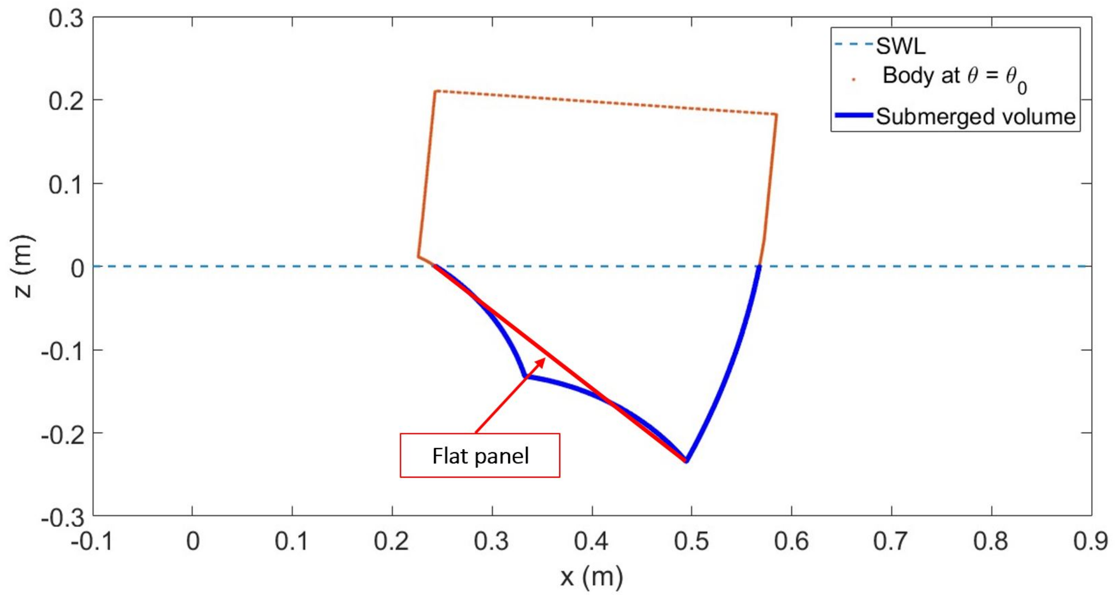
Approximated formulation of quadratic drag forces

In order to simplify and improve the computational efficiency, three simplifications to Equation (22) are applied. The first simplification is that the instantaneous submerged body surface area is approximated by single flat panel (Figure 4). The second simplification is that the fluid velocity is neglected. The third simplification is that the drag forces are only computed when the WEC is pitching clockwise (when the WEC rotates in the opposite direction the projected area is small hence the quadratic drag forces can be neglected).

Applying these three simplifications, Equation (22) reduces to,

$${\overrightarrow{F}}_{drag}=-{\displaystyle \frac{1}{2}}\rho C_d{\overrightarrow{S}}_p^{*}\dot{\overrightarrow{x}}\parallel \dot{\overrightarrow{x}}\parallel ,$$

(27)

where ${\dot{x}}_i$ represents translational velocity of the centroid of the single panel in the $(x^{\prime },y^{\prime },z^{\prime })$ directions and $S_p^{*}$ is the projected surface area of the flat panel.

3.3.6. Friction in the Bearings, $M_{fb}$

The friction moment in the bearing around the rotation shaft can be modelled as dry friction. The friction in the bearings is approximated as a constant moment of magnitude $K_{fb}$, opposing the WEC’s motion:

$$M_{fb}=-K_{fb}sign\left(\dot{\theta }\right).$$

(28)

3.3.7. Numerical Model Solver

The equation of motion is solved in the time domain in Simulink using a fixed-step ODE3 solver with fixed-step size of 0.001 s. Inputs and outputs are processed in Matlab.

4. Wave Basin Experiments

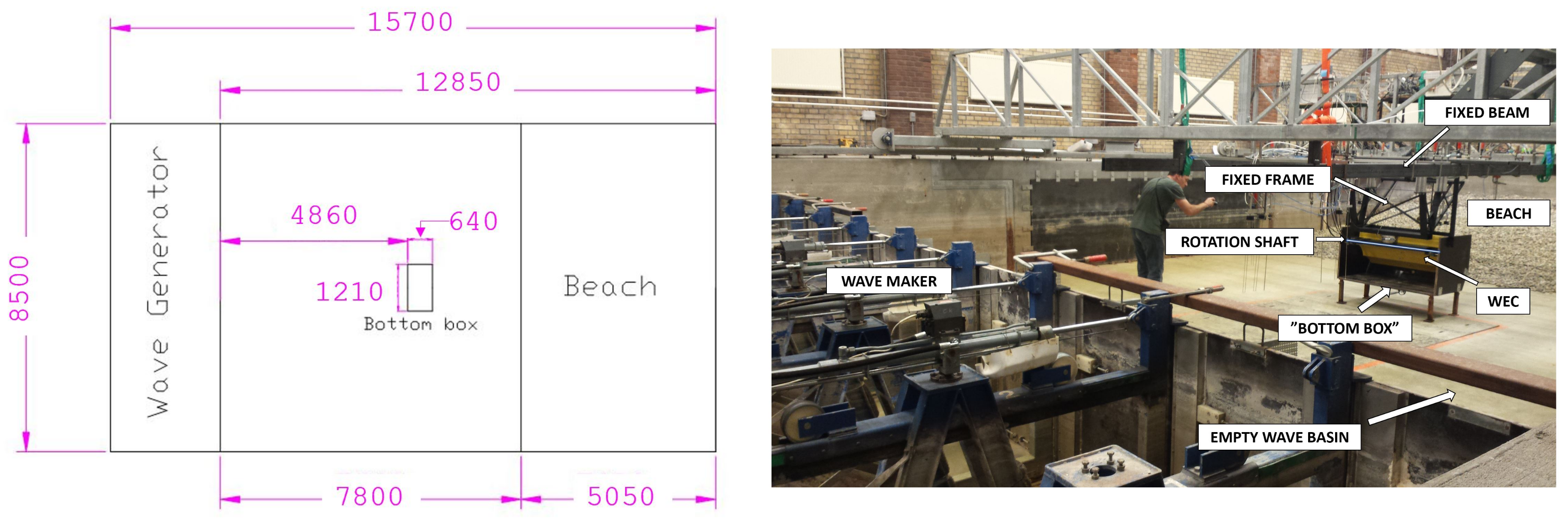
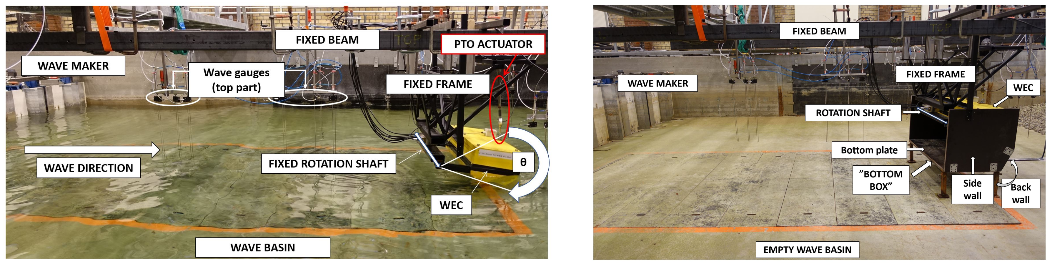
4.1. Laboratory Setup

The data used for model validation in this paper comes from 1:30 scaled tests performed at Aalborg University in “The deep 3D wave basin”. The scaled model WEC is a 1:30 simplification of a double-width full-scale WEC. The main dimensions of both the FPP conceptual design and scale model WEC are included in

Table 1. Main dimensions of FPP conceptual design and model scaled WEC.

Semisubmersible			WEC			WEC Scale Model
Length main body	86.5 m		Length main body	10.8 m		Length main body	343.5 mm
Length hinged arms	99.3 m		Width	18.3 m		Width	1105.0 mm
Width	36.0 m		Height	11.0 m		Height	423.0 mm
Height	25.0 m		Length hinged arms	6.2 m		Length hinged arms	228.5 mm
Water depth	>45.0 m					Water depth	650.0 mm

. In the wave basin setup, the distance between the rotation shaft and the bottom box is 400 mm, the bottom plate is 1210 mm wide and 640 mm long, the gap between the side walls and the WEC is 36 mm and the clearance between the back of the WEC and the inclined back wall is 20 mm. The inclined back wall is 214 mm high measured from the horizontal surface of the bottom box (“bottom plate”), so it does not protect the back of the WEC from wave reflections from the beach. For confidentiality reasons, more detailed information about the geometry and physical properties is not provided.

The wave basin has the dimensions of 15.7 m long, 8.5 m wide and 1.5 m deep. Dimensions of the wave basin and location of the WEC are shown in Figure 5.

The wave elevation is measured by 16 wave gauges that are placed in the basin, see Figure 6. Twelve wave gauges are placed along the centre line of the basin: 6 in front of the WEC, numbered 1–6 (2 pairs of 3 gauges); and 6 behind the WEC, numbered 11–16 (2 pairs of 3). The setup, with the multiple wave gauges along the centre line, allows for accurately separating incident and reflected waves using 2D wave analysis (along the length of the basin). The remaining 4 wave gauges, numbered 7–10, are placed by the side of the WEC, which allows for the investigation of 3D effects of diffracted and radiated waves (across both the length and the width of the basin).

Figure 7 shows the setups of two test configurations that are used for experimental validation in this paper. In both configurations, the rotation shaft for the WEC is fixed in space by attachment to a fixed beam (Figure 7). The first configuration (WEC only), consists of the WEC alone. The second configuration (WEC+BB) includes, in addition, the fixed substructure, also called “bottom box” or “BB”. The bottom box consists of two side-walls, a back wall and a bottom plate. The width of the WEC is 1105 mm and the clearance between the inner surface of the side-wall and the outer sides of the WEC (port and starboard) is 36 mm.

4.2. Wave Basin Experimental Data

The different tests performed for the validation and comparison of the numerical model versions include:

4.2.1. Undisturbed Waves

When waves are generated in the basin, some reflection effects from the beach occur. In order to decompose the measured free surface elevation into incident and reflected waves at the WEC position, the following procedure is used:

• Waves are generated and measured in the basin without the WEC in place (undisturbed waves) using the software “Awasys” from Aalborg University, including active absorption.
• A non-linear wave analysis is performed to separate incident and reflected waves using the software “WaveLab” from Aalborg University [28]. WaveLab takes into account the propagation speed of the waves in a non-linear manner.
• The same waves are then repeated with the device in position.

4.2.2. Slow-Motion Experiments

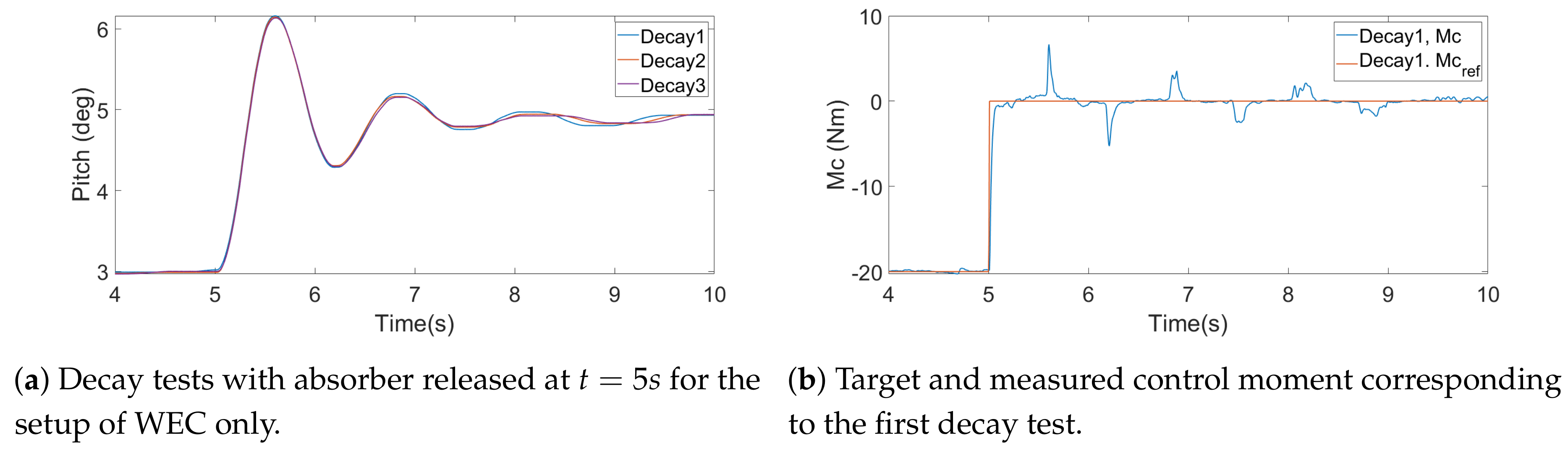
The WEC is moved gently up and down and simultaneous measurements of the position and control moment are acquired. The WEC is moved with a constant velocity of 0.24 deg/s using the actuator.

4.2.3. Decay Tests

The WEC is lifted (or pushed down) using the actuator, which is set to provide a constant moment in order to keep the WEC away from its static position for a few seconds before releasing it. An example of a (repeated) decay test is shown in Figure 8a. As illustrated, when repeating the decay tests for the same conditions, very similar motions are observed. The difference between target and measured moment provided by the actuator is presented in Figure 8b, where the irregularities in the measured moment are due to friction effects.

4.2.4. Fixed WEC Experiments

The actuator applies a control moment to the WEC in order to obtain a fixed target position despite the influence of the incoming waves. The target position corresponds to the static, neutrally-buoyant position of the WEC. The measured control moment during these tests is directly the wave excitation moment [29].

The non-linear model calculates Froude-Krylov moment defined in Equation (18) with $P_{dyn}$ calculated as either $P_{dyn}^{\left[1\right]}$ (Equation (16)) or $P_{dyn}^{\left[2\right]}$ (Equation (17)). Where $P_{dyn}=P_{dyn}^{\left[1\right]}$ (non-linear model), the submerged body geometry is calculated at the instantaneous rotation angle (${\theta }_i$). Where $P_{dyn}=P_{dyn}^{\left[2\right]}$ (non-linear model with Wheeler stretching), the submerged body geometry is calculated at the instantaneous position (${\theta }_i$). In the non-linear model, the scattering moment is interpolated for the instantaneous angle of the WEC.

Using the formulation to calculate excitation moments that considers the instantaneous body position of the WEC (non-linear model) supposes a difference in amplitude of the excitation moment compared to linear theory of up to 4%. This difference goes up to 7% when Froude-Krylov formulation includes Wheeler stretching as well.

The comparison between excitation moments in free motion simulations is done for regular waves with wave period equal to the resonant period of the WEC and for two wave heights—the one used as target wave height for the experiments, and a wave height two times bigger. Time-series of the results are included in Figure 9 and normalized results by the wave amplitude are included in Figure 10. The largest wave height makes the WEC to rotate within the limit angles that allow it to not leave the water and to keep the top surface out of the water in order to facilitate the numerical modelling.

4.2.5. Regular Waves

The undisturbed waves, wave excitation and free motion experiments are performed for 16 different regular waves with periods between 0.667 and 2.5 s with a target wave height of 4 cm, defined in

Table 2. Regular waves used for undisturbed waves, fixed WEC and free motion in regular waves experiments.

Wave condition	R01	R02	R03	R04	R05	R06	R07	R08
$\mathbf{T}$ (s)	2.500	2.000	1.667	1.429	1.250	1.176	1.111	1.053
$\mathbf{H}/\mathbf{2}$ (m)	0.019	0.020	0.019	0.019	0.019	0.019	0.020	0.021
Wave condition	R09	R10	R11	R12	R13	R14	R15	R16
$\mathbf{T}$ (s)	1.000	0.952	0.909	0.870	0.833	0.769	0.714	0.667
$\mathbf{H}/\mathbf{2}$ (m)	0.021	0.023	0.021	0.022	0.021	0.021	0.023	0.023

. Figure 11 shows how these waves are classified according the applicability of wave theories defined in [30]. In the figure, the ratio between the parameters $H_0/\left(g{T}_p^2\right)$ and $d/\left(g{T}_p^2\right)$ indicates that all the waves are non-linear, belonging to the region where the suitable wave theory is Stokes 2nd order, except from the 3 shortest waves, that correspond to Stokes 3rd order. The ratio between water depth d and wavelength $\lambda$, shows that the waves used in these experiments correspond to either intermediate water depth or deep-water definition, and the relation between wave height and wavelength indicates the steepness of the wave. None of the waves included in the tests correspond to the linear theory description, thus stressing the objective of this paper, which is to check the suitability of a numerical model based on linear potential wave theory.

Figure 12 illustrates the measured experimental data used. The first subplot includes the calculated incident and reflected waves at a position vertically below the hinge. The incident and reflected waves have been calculated using WaveLab using the wave gauges data from the undisturbed waves experiments. The second subplot, data from the free motion experiments in regular waves. Finally, the third one, from the wave excitation experiments. All three experiments are performed for the same target wave.

4.2.6. Free Motion in Regular Waves

The WEC is allowed to move freely in the waves, without the addition of a control moment. Figure 13 illustrates a frequency domain comparison of the response amplitude operator (RAO) obtained using the different models. The RAO represents the ratio between the amplitude of motion and the wave amplitude. The numerical model that considers linear hydrodynamic forces (“Linear”, blue dotted line in Figure 13) calculates Froude-Krylov forces using Equation (16) for the hydrostatic rest position of the WEC and Equation (18), scattered forces as in Equation (19) for the rest angle, and gravity and buoyancy forces as in Equations (12) to (15), again for the hydrostatic rest position. The second version of the numerical model is a linear numerical model that includes in addition the approximated quadratic drag that is given by Equation (27) (“Quasi-linear”, rust-coloured dotted line in Figure 13). Finally, results from a non-linear model are included for comparison (“Non-linear”, yellow-dotted line in Figure 13). The non-linear numerical model considers instantaneous forces stand for formulation of Froude-Krylov forces as in Equations (17) and (18), scattered forces as in Equation (19) for the instantaneous WEC position, buoyancy force as in Equations (13) to (15) for the instantaneous WEC position, gravity force as in Equation (12) for the instantaneous WEC position, and the exact formulation of the quadratic drag force defined by Equations (22) to (26).

The biggest difference between numerical models corresponds to the natural period of the WEC. The numerical model that includes linear forces and the simplified version of quadratic drag force (“Quasi-linear”) introduces an overestimation in motion of up to 12% compared with the most exact model (“Non-linear”) for the wave conditions simulated, but it is 20 times faster. Simulating 10 s of WEC motion takes 7.5 s using the quasi-linear model, whilst it takes 150 s using the non-linear one. The computational effort of the quasi-linear numerical model makes it to be the most optimal even though the calculated motions can have an error of up to 12% compared to the non-linear model.

4.2.7. Quadratic Drag Moment

The approximated formulation of the quadratic drag moment included in the quasi-linear model provides a good match with the more exact formulation included in the non-linear model, as Figure 14a shows. The simplification of the quadratic drag forces has a negligible effect in the pitch motion. Figure 14b presents the sensitivity of the quasi-linear model to the drag coefficient value. The |RAO| curves presented in this figure are calculated from time domain simulations using the fast Fourier transform to both the free surface and the pitch motion, and then calculating their ratio. The simulated theoretical regular waves are defined by the parameters included in Table 2.

5. Results

5.1. Wave Reflections and Repeatability

Wave reflections in the basin and the repeatability of the wave generation are important. The presence of the WEC affects the waves in the basin due to reflections, and also the motions of the WEC influences the waves due to radiated waves. In addition, the wave generator is not perfect in reproducing the waves (although the standard deviation of the significant wave heights for tested waves is only 0.3%). In order for these effects to have minimum influence on the results, the actual measured waves in each test are used. For this purpose, data measured by all the wave gauges is used to calculate the incident and reflected wave time series at specified positions (i.e., at the origin of the coordinate system of the WEC, which is at the centre of the bearing) using WaveLab.

Figure 15 presents data from one of the wave gauges during three different experiments under regular waves conditions: undisturbed waves, fixed WEC with WEC only and fixed WEC when the bottom box is installed as well. Figure 15a shows how the waves are affected by the presence of bodies in the basin. For the first seven seconds, the measured waves are very similar due to the capability of repeatability of the wave maker. After this initial time, diffracted and reflected waves make the measurements disagree between experiments. In order to simplify the validation of the numerical model process, only heading waves are considered. The measured data used for validation is chosen from the interval of time where there are no reflected waves from the beach of the wave basin. Figure 15b presents the calculated incident wave after performing the reflection analysis with WaveLab. The results from WaveLab show good agreement between the calculated incident waves for two different experiments (undisturbed waves and fixed WEC) for the first part of the experiments where wave reflections have not occurred yet or are negligible.

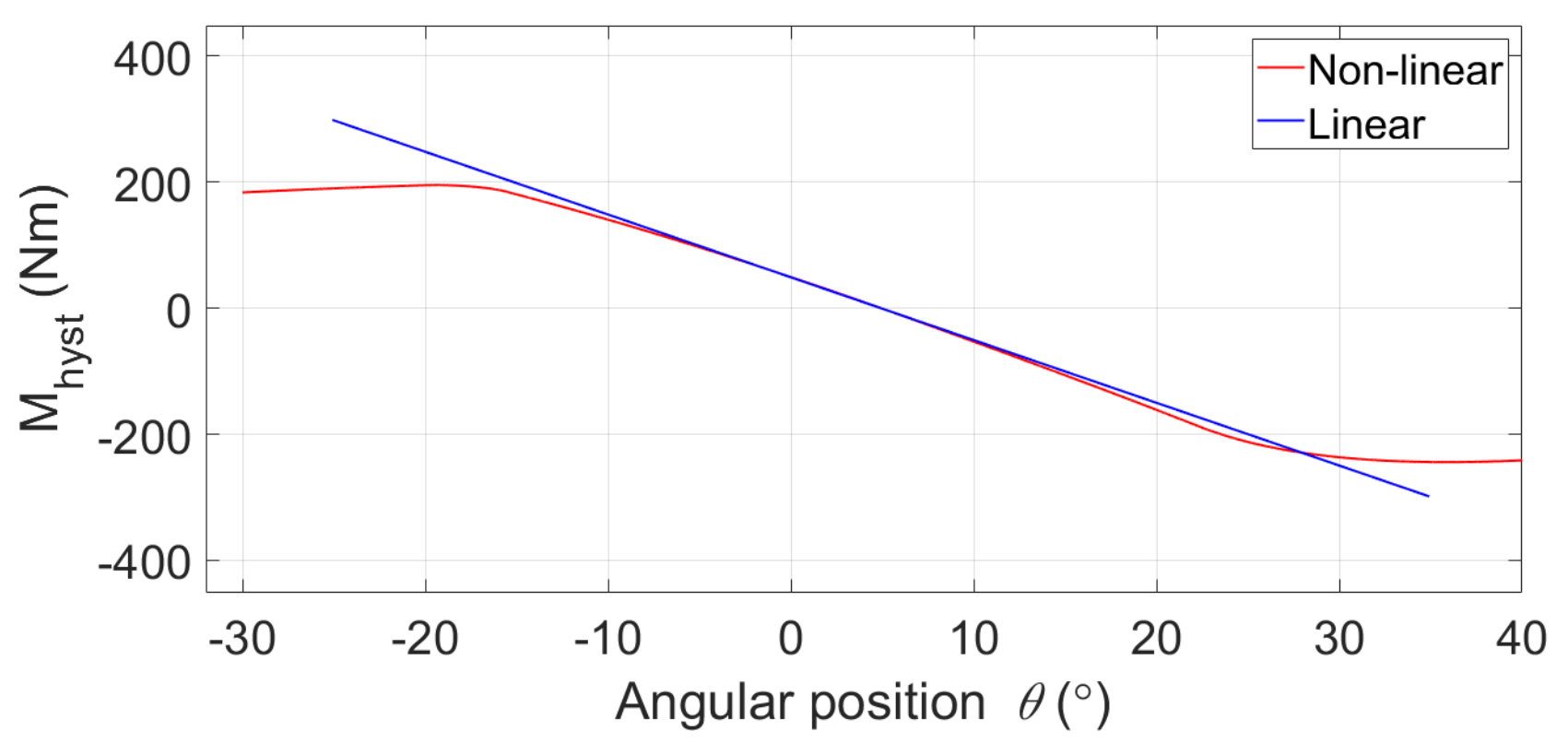
5.2. Modelling of Hydrostatics and Friction

The hydrostatic stiffness is close to linear with the WEC angle for angles of inclination between −5 and 10 degrees (maximum 2% discrepancy), see Figure 16. However, excluding the situations where the WEC is either fully submerged or out of the water (where the hydrostatics become more constant), the assumption of linear hydrostatics is reasonable (maximum 10% discrepancy at the highest angle of inclination). The hydrostatic rest position corresponds to the angular position with zero hydrostatic moment. In this case the rest angle is ${\theta }_0=4.9$ degrees.

During the slow-motion tests, the acceleration is zero and the velocity is constant but negligible, as seen in Figure 17a. Under these conditions, the dynamic equation of motion (Equation (5)) reduces to

$$-M_c=M_{grav}+M_{buoy}+M_{fb}.$$

(29)

The exact measured moment, $M_c$, at a specific angle during the slow-motion tests depends on the direction of rotation, up to 2 Nm deviation (see Figure 17b, where the double green line represents measured data in both directions of rotation of the WEC). The dependence on the direction of rotation comes from dry friction (Equation (28)) and possibly also due to small variations in $M_{grav}$, since the rotation of the WEC affects the position of connection cables, making them lie more or less on the device and affecting its weight [31]. The magnitude of the variations in $M_{grav}$ is unknown, so Equation (29) is satisfied for values of $K_{fb}$ between 0.4 and 1 within $M_{fb}$ (Equation (28)). These values of $K_{fb}$ are estimated based on the experimental data.

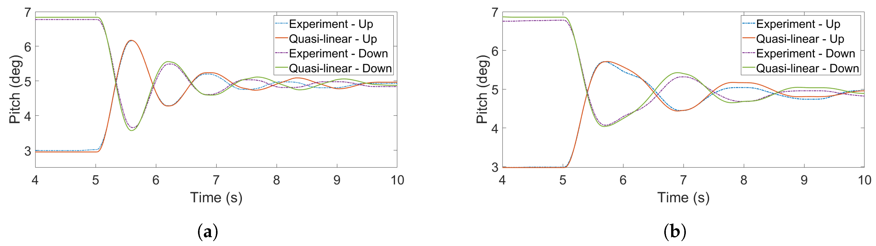
5.3. Decay Tests Simulations

In decay tests, there is no excitation moment due to waves, hence Equation (5) reduces to

$$J{\ddot{X}}_5=M_{grav}+M_{buoy}+M_{rad}+M_c+M_{drag}+M_{fb}.$$

(30)

The pitch motion calculated using Equation (30) with values of $C_d=2$ within $M_{drag}$ (Equation (27)) and $K_{fb}=0.4$ within $M_{fb}$ (Equation (28)) results in close match to experimental measurements (Figure 18). The value of $C_d=2$ has been chosen to provide a good match with experimental data and taking as reference values found in literature [32]. The influence of the friction in the bearing is presented in Figure 19a.

The hinge height, which is the origin of the body coordinate system, is fixed relative to the seabed with a target height of 50 mm above the still water surface. A difference in hinge height of 1 mm actually corresponds to an accuracy in this hinge height of $\pm 2$%. This accuracy corresponds to a change in rest angle of about $\pm 0.15$ degrees and impacts the hydrodynamics. The location of the hinge is fixed in space throughout all the experiments. However, the hinge height relative to the water level varies by up to 2 mm due to daily variations in water depth in the wave basin (due to leakage). Figure 19b shows how 1 mm of difference in water depth affects the simulated motion of the WEC. The accuracy in the manual measurements and the differences due to changes in water depth is estimated to be $\pm 1$ mm. The variations in water depth result in the slight differences between the modelled and experimental initial positions (Figure 18a,b).

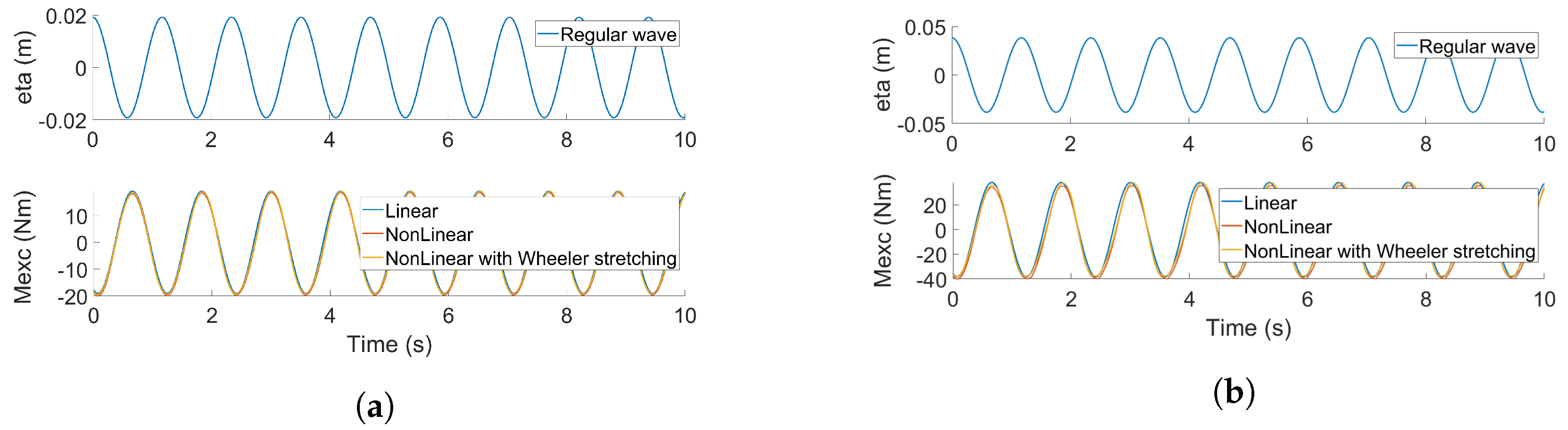
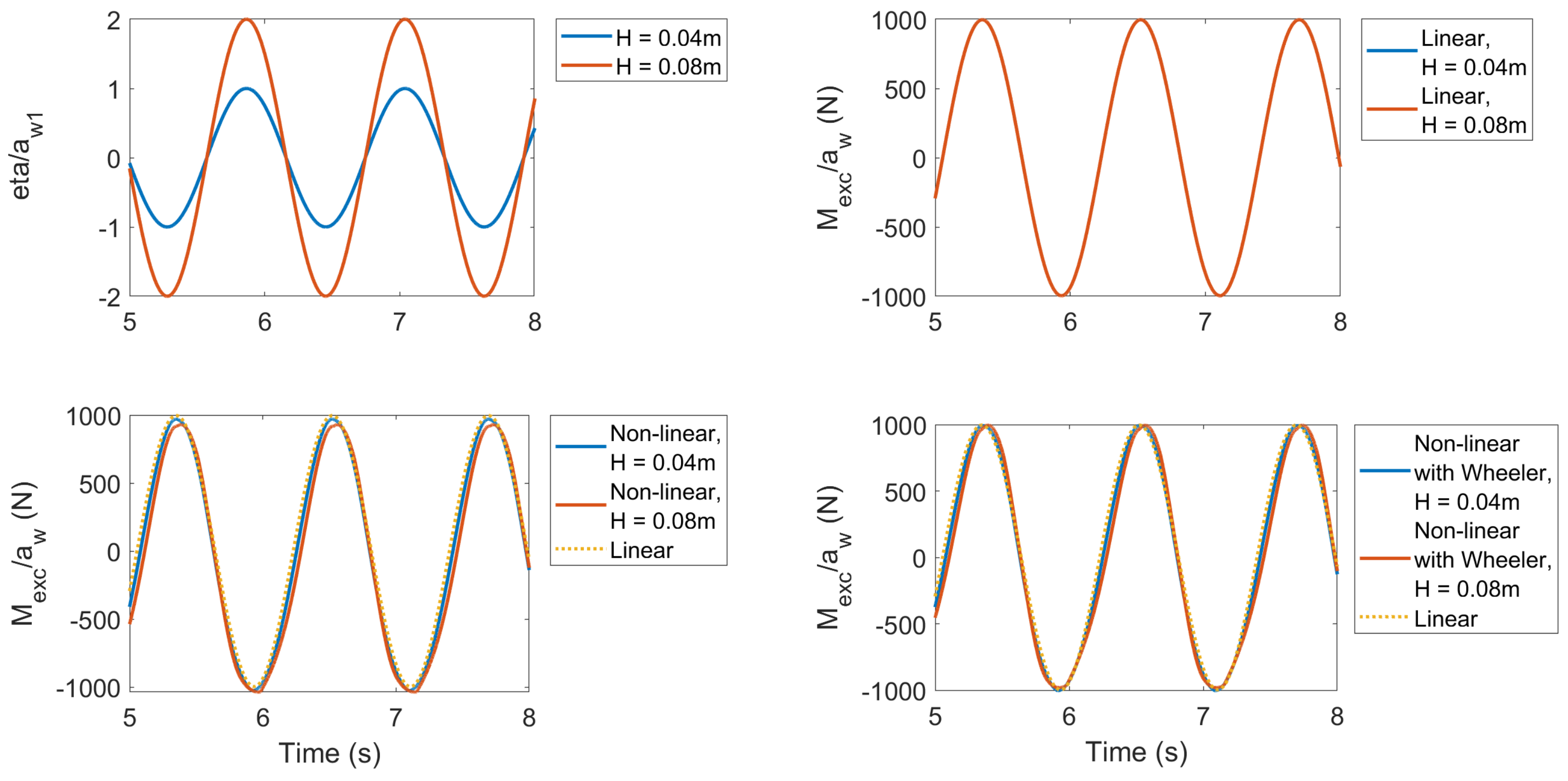
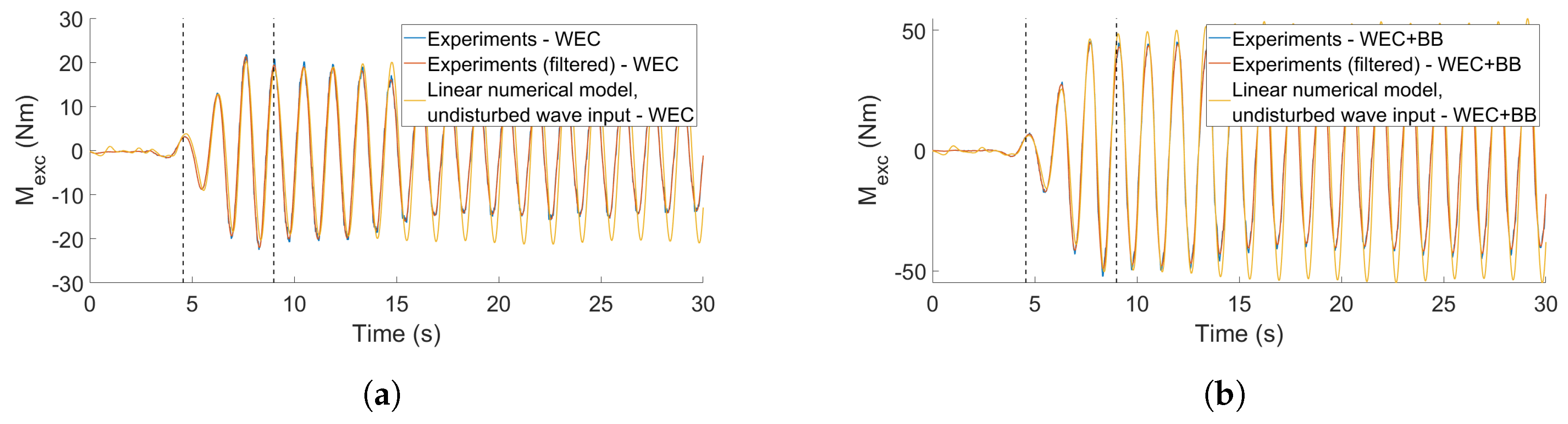
5.4. Wave Excitation

When the WEC is held fixed at a constant angle of inclination by the actuator, the dynamic equation of motion (Equation (5)) reduces to

$$-M_c=M_{grav}+M_{buoy}+M_{exc}.$$

(31)

During these tests, the WEC is held at the hydrostatic rest position by the actuator. Hence, the buoyancy and gravity moments cancel each other and the moment provided by the actuator is equal to the excitation moment.

Excitation loads can be defined as the sum of Froude-Krylov and scattering loads. Froude-Krylov loads are based on the formulation of the dynamic pressure on the WEC surface according to linear theory, and therefore it is the same for the setup of WEC only and for WEC+BB. Scattering loads are however different, making total excitation loads different as well. Figure 3 includes results from WAMIT, showing that excitation forces are larger for the setup of WEC+BB, being the scattering force contribution dominant over Froude-Krylov for the whole range of periods in this case.

The model used for comparison of excitation forces with experimental data is based on linear formulation. Froude-Krylov and scattered moments are calculated based on the submerged volume at the hydrostatic rest position defined by the still water line. To simulate the experiments, only the undisturbed heading incident wave is taken into account, neglecting the reflection from the back of the wave basin of both incident and scattered waves. Due to the simplification of neglecting reflected incident and scattered waves, it is only reliable to compare the simulations with the measured excitation signal recorded before reflection occurs. In this time window, a good match between experimental data and the linear model is found for regular waves (Figure 20), being the time window chosen for comparison represented by the vertical dashed lines.

Time domain results are useful for comparison and validation with numerical modelling. A frequency domain representation of the simulations under regular waves conditions is done by calculating the ratio between the mean of the amplitude the excitation moment and the mean of the amplitude of the wave amplitude in the time window where reflection is negligible. The amplitude of the excitation moment and the wave amplitude are calculated through a “peak analysis”, by using the peaks and the troughs of the signals in the selected time window. Fast Fourier transform is not applied because the un-contaminated timeseries are extremely short, and frequency analysis in this interval does not provide realistic results. The frequency domain representation of the results from the “peak analysis” (Figure 21) can be misleading, specially for long waves. This is because results for long periods are based on short time windows, where very few oscillations are considered and the steady state has not been reached.

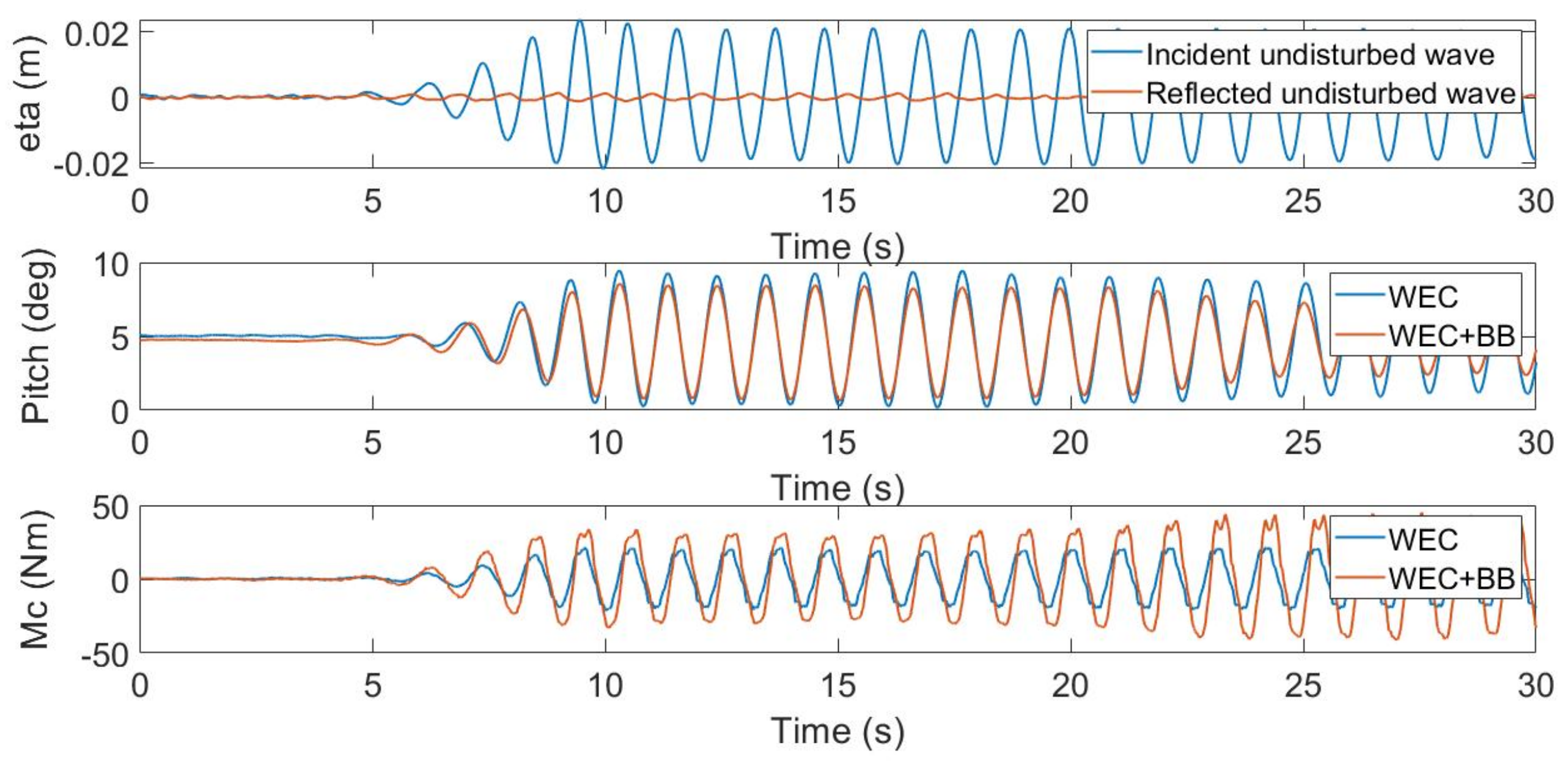
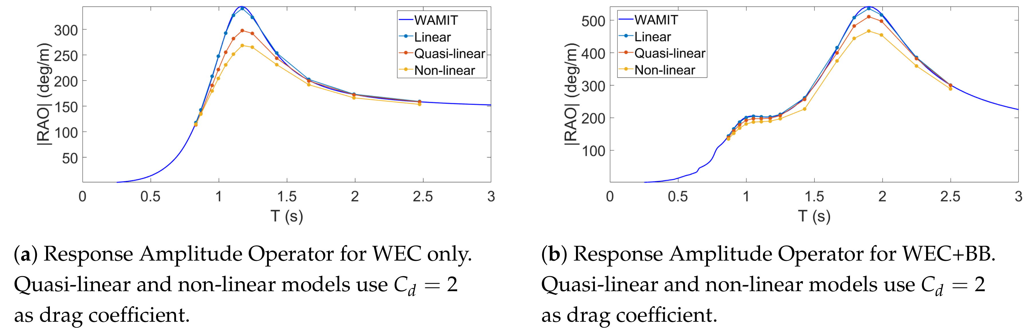
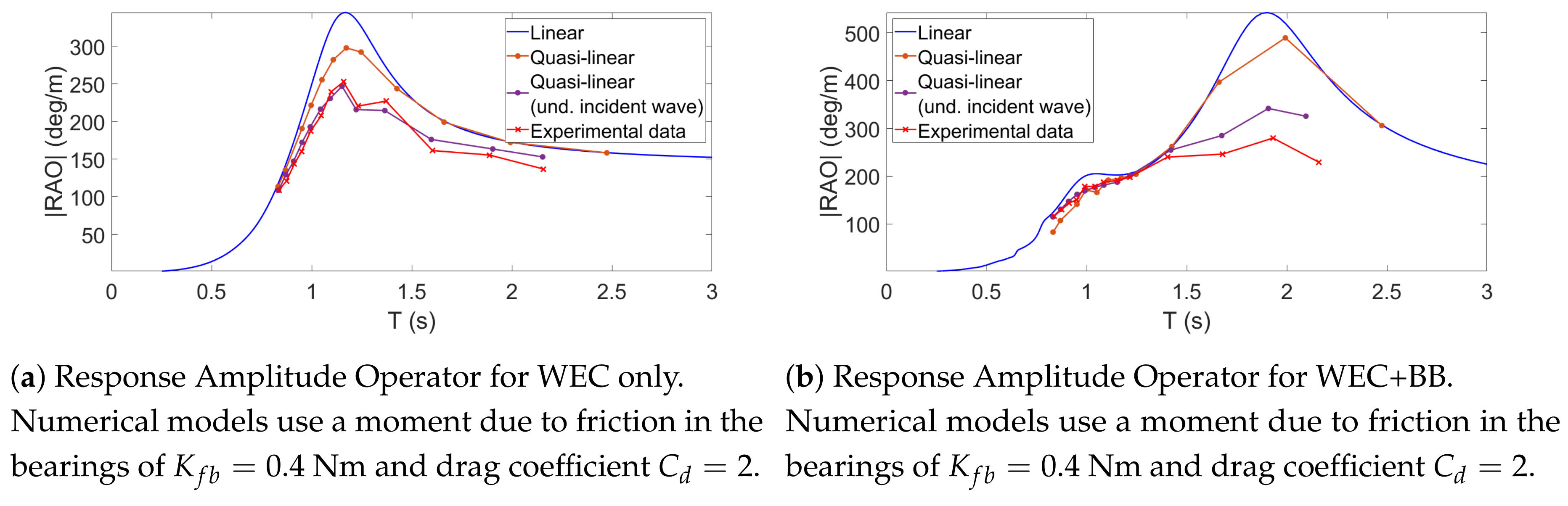
5.5. Free motion in Regular Waves

The linear model has shown a good match with wave excitation experiments. During free motion tests, wave excitation was not measured. But in this section the different numerical formulations are compared.

The quasi-linear model showed that formulating moments with a linear approach translates into an overestimation in motion. Even though this error appears to be large in the frequency domain as shown in Figure 13, time domain comparison with experimental data shows an acceptable agreement in motion amplitudes although a small phase shift occurs (Figure 22). However, for the setup of WEC with bottom box, for the second natural frequency of the WEC calculated by linear theory (2 s), the error in time domain is more noticeable (20%), as illustrated in Figure 23. This percentages differ from those mentioned before because when using experimental data, for the long periods, the data used does not correspond to steady state and that is a source of error to add to all the errors due to the simplifications that the linear numerical considers.

Data 4 extra experiments of free motion in regular waves with the wave conditions defined in

Table 3. Regular waves used for free motion in regular waves experiments in order to analyse the influence of increasing wave amplitude.

Wave condition	R09	R17	R18	R19	R20
$\mathbf{T}$ (s)	1.00	0.95	0.98	0.99	0.98
$\mathbf{H}$ (m)	0.042	0.020	0.059	0.076	0.092

is available for validation. Results from the quasi-linear model are compared to the measured motion in Figure 24. Two different values of the quadratic drag coefficient are used in these simulations. The effect of the quadratic drag coefficient in time domain is less noticeable than in the frequency domain (Figure 14b). Unfortunately, data from fixed-WEC experiments is not available, so a comparison of the excitation moments cannot be done.

To summarize the results of free motion in regular waves for both wave basin setups, (with and without bottom box), the response amplitude operators corresponding to each regular wave tested are included in Figure 25. The values of the amplitude of the RAO are calculated using the data within time interval where the reflection is considered negligible. Examples of these time windows are shown in Figure 22 and Figure 23. The peaks and the troughs of the wave amplitude and the WEC motion in this interval are used to calculate the ratio between the mean values of the pitch motion and wave amplitude (|RAO|).

As seen in Figure 25, the quasi-linear model gives different results depending on the input wave. When using the undisturbed incident wave from the experiments, the RAO amplitudes decrease significantly for long waves in comparison to linear theory, specially for the case of WEC with bottom box. This is because the data used to calculate the RAO is reduced to a time window where the wave is not fully developed and behaving in a non-linear manner, thus results are less reliable than those that come from fully developed waves that behave in a more linear way. However, considering the actual experimental wave makes the numerically calculated response to be more similar to the experimental one, although still for long waves the difference between experimental and calculated RAO amplitude is 40% for the longest period and 22% for the second longest period for the simulated wave conditions.

6. Discussion

The numerical model solves the dynamic equation of motion of a pitching WEC, with and without a bottom-fixed second body. Linear, quasi-linear and non-linear formulations of hydrodynamic forces and motions were compared against each other and against experimental data when possible. Experimental data is key to deciding which numerical model is more suitable for the case study regarding both efficiency and accuracy. Due to the nature of laboratory experiments, there are some uncertainties that make the exact determination of inputs to the numerical model difficult. The input that affects the numerical model the most is water depth, since a 1 mm change in water depth alters the angle of inclination of the WEC by $\pm 0.15$ degrees. This small change in angle affects the hydrostatics of the system, as well as the hydrodynamics.

Hydrostatic stiffness was compared to results from slow-motion tests, added mass and radiation damping to decay tests and wave excitation moments to fixed-WEC tests. In all these cases, results from linear formulations, with the inclusion of an approximated formulation of quadratic drag for decay tests, showed good agreement with measured moments despite the atypical body geometry. For linear regular waves, the maximum difference in motion relative to the incoming wave between the quasi-linear model and the non-linear was less than 12%. However, the quasi-linear model, for which the computational effort is similar to the linear model, was 20 times faster than the non-linear one. The quasi-linear model provides a close match to experimental data for the pitch motion of the WEC, provided the WEC is alone in the wave basin. However, when the fixed substructure is in place, the model overestimates the body motion for the longest waves tested (maximum 40%).

The experimental data used for comparison is less reliable for the case of long waves due to reflection effects. Other codes like WEC-Sim, based on the same formulations as the models presented in this paper, have been validated and calibrated [14,16,33] using wave basin experiments as well. However, the published results do not include an experimental validation as complete as that presented in this paper, which makes it difficult to use WEC-Sim for code to code comparison.

Although some reasons for the over-prediction of motion in long waves could be unreliable data, viscosity or friction, it could also be due to resonance effects of the water trapped between the two bodies. This resonance might magnify the forces acting on the bodies and, in this case, it would be needed to include extra damping due to viscous effects to absorb this resonant energy. To improve the agreement between potential theory and experimental data, some methods like the addition of flexible lids on the free surface inside the gaps have been studied in [34]. The value of the damping parameter that define these lids should be provided by experimental data. In addition, these flexible lids may affect the excitation, added mass and radiation damping coefficients computed by the software WAMIT, so excitation and radiation experiments are also required to confirm these values. Gap resonances have been investigated in other studies, mainly for cases of side-by-side vessels, highlighting the dominating linear behaviour of the system for the scaled geometries tested, and establishing a method to scale linear viscous damping for different gap widths [35]. These approaches should be further studied.

The experimental data used in this paper is of extraordinary high quality; even so, some more experiments could aid a deeper understanding of the behaviour of the device and validation and/or calibration of the model. Some suggested tests are radiation tests, decay tests with different starting positions, or free motion in regular waves with increasing steepness values for different wave periods. Measurements of the water surface elevation in the gaps and over the bottom plate are also crucial to determining resonances caused by the interaction between bodies.

7. Conclusions

Experimental data is crucial for validation of numerical models. This paper presents the method used to validate a model of the dynamic equation of motion of a pitching body based on the validation of the individual moments using experimental tests. Buoyancy and gravity moments were validated with slow-motion tests, showing a good match. Decay tests were used to validate radiation moment at the natural frequency of the body and to quantify the friction in the bearings. Excitation moments were validated using tests where the WEC was fixed, which allows for validation of these moments at static position. The input wave to the numerical model strongly influences the model outputs. It is therefore important to take care choosing the input wave and the time interval of experimental data to compare against in order to validate the model. The experiments were planned with the main purpose of numerical model validation, resulting in a high-quality dataset. However, testing in a wave basin has some limitations and the most significant one in this case was that long waves are difficult to test in this facility. Waves reflected at the beach reach the device before the waves are fully developed, so the system does not reach a steady state. During the time that it takes for the waves to be fully developed, the data corresponding to long waves is more difficult to interpret and use for validation. Unfortunately, it is in this range of frequencies where interesting dynamic interactions occur between the pitching body and the fixed surrounding substructure.

Linear, quasi-linear and non-linear models were considered in this paper. The non-linear model includes gravitational, buoyancy, Froude-Krylov, scattered and quadratic drag moments calculated for the instantaneous body position. The wave kinematics were extended above the still water line in the calculation of buoyancy and Froude-Krylov moments. The formulation of the scattered moment was approximated by the steady state moment for the instantaneous angle. The quasi-linear version calculates moments in a linear manner except quadratic drag loading. The maximum difference (less than 12%) between the RAO (Response Amplitude Operator) of the non-linear model and the quasi-linear model is at the resonant frequency when simulating theoretical regular waves. The non-linear model presented requires the fluid velocity profile to be known across the body surface at each time step. Since the experimental waves are not sinusoidal this calculation is time consuming. Only the linear and quasi-linear models were therefore used for data comparison. Despite the non-conventional geometry of Floating Power Plant’s WEC, comparison to measured data shows that its behaviour is unexpectedly linear. Linear theory captures the trends of the WEC’s motion with frequency but not amplitude.

The quasi-linear numerical model (linear model with an approximated quadratic drag) is recommended as a good balance of accuracy and efficiency for the wave conditions tested. The quasi-linear model overestimates the motion of the pitching WEC when there is a surrounding fixed substructure and long waves are simulated (40% for the longest way tested and 22% for the second longest one). Yet, the quasi-linear model provides a good match with experimental data in all other cases. As has been explained before, the long waves provide a very short time window of quality data, so these results may not be totally reliable for validation. The author expects this overestimation to be slightly reduced (up to 12%) if the non-linear model is used, yet the computationally effort would be 20 times larger. It is indicative that the quasi-linear model is working, but simulations and comparison with experimental data for larger wave amplitudes have to be done in further studies to prove it. Potential phenomena causing the mismatch between numerical and experimental data could be the dynamically varying gap between the two bodies, which could imply the need to include a dynamic formulation of scattered forces, resonance effects of the water surface between the two bodies and/or uncertainty on physical parameters such as bearing friction. More research is required to identify the causes of the multi-body interaction effects for long waves.

References

1. Weber, J. WEC technology readiness and performance matrix—Finding the best research technology development trajectory. In Proceedings of the 4th International Conference on Ocean Energy, Dublin, Ireland, 17–19 October 2012. [Google Scholar]
2. Falnes, J. Principles for Capture of Energy from Ocean Waves. Phase Control and Optimum Oscillation; Department of Physics, NTNU, N-7034: Trondheim, Norway, 1997. [Google Scholar]
3. Salter, S.H. Wave power. Nature 1974, 249, 720–724. [Google Scholar] [CrossRef]
4. Pecher, A.F.S.; Kofoed, J.P. (Eds.) Handbook of Ocean Wave Energy; (Ocean Engineering and Oceanography series, Vol. 7); Springer: Cham, Switzerland, 2017; 287p. [Google Scholar]
5. Floating Power Plant. Available online: http://floatingpowerplant.com/ (accessed on 10 January 2019).
6. Bellew, S.; Yde, A.; Verelst, D.R. Application of the aero-hydro-elastic model hawc2-wamit, to offshore data from floating power plants hybrid wind and wave energy test platform p37. In Proceedings of the 5th International Conference on Ocean Energy (ICOE), Halifax, NS, Canada, 4–6 November 2014. [Google Scholar]
7. Yde, A.; Larsen, J.; Hansen, A.M.; Fernandez, M.; Bellew, S. Comparison of simulations and offshore measurement data of a combined floating wind and wave energy demonstration platform. J. Ocean. Wind. Energy 2015, 2, 129–137. [Google Scholar] [CrossRef]
8. OES Task 10: Wave Energy Converters Modelling Verification and Validation. Available online: https://bit.ly/2zv0ebb (accessed on 10 January 2019).
9. Wendt, F.F.; Yu, Y.H.; Nielsen, K.; Ruehl, K.; Bunnik, T.; Touzon, I.; Nam, B.W.; Kim, J.S.; Janson, C.E.; Jakobsen, K.R.; et al. International Energy Agency Ocean Energy Systems Task 10 Wave Energy Converter Modeling Verification and Validation. In Proceedings of the 12th European Wave and Tidal Energy Conference (EWTEC), Cork, Ireland, 27 August–1st September 2017. [Google Scholar]
10. Folley, M. Numerical Modelling of Wave Energy Converters: State-of-the Art Techniques for Single WEC and Converter Arrays; Elsevier: Amsterdam, The Netherlands, 2016; ISBN 978-0-12-803210-7. [Google Scholar]
11. Babarit, A.; Mouslim, H.; Clément, A.; Laporte Weywada, P. On the Numerical Modelling of the Non Linear Behaviour of a Wave Energy Converter. In Proceedings of the ASME 2009 28th International Conference on Ocean, Offshore and Arctic Engineering, Honolulu, HI, USA, 31 May–5 June 2009. [Google Scholar] [CrossRef]
12. Wolgamot, H.A.; Fitzgerald, C.J. Nonlinear hydrodynamic and real fluid effects on wave energy converters. Proc. Inst. Mech. Eng. Part J. Power Energy 2015, 229, 772–794. [Google Scholar] [CrossRef]
13. Giorgi, G. Nonlinear Hydrodynamic Modelling of Wave Energy Converters under Controlled Conditions. Ph.D. Thesis, National University of Ireland Maynooth, Maynooth, Ireland, 2018. [Google Scholar]
14. Ruehl, K.; Michelen, C.; Yu, Y.-H.; Lawson, M. Update on WEC-Sim Validation Testing and Code Development. In Proceedings of the 4th Marine Energy Technology Symposium, METS 2016, Washington, DC, USA, 25–27 April 2016. [Google Scholar]
15. Combourieu, A.; Lawson, M.; Babarit, A.; Ruehl, K.; Roy, A.; Costello, R.; Laporte Weywada, P.; Bailey, H. WEC 3: Wave Energy Converter Code Comparison Project Preprint. In Proceedings of the 11th European Wave and Tidal Energy Conference, Nantes, France, 6–11 September 2015. [Google Scholar]
16. Ruehl, K.; Michelen, C.; Bosma, B.; Yu, Y.-H. WEC-Sim Phase 1 Validation Testing—Numerical Modeling of Experiments. In Proceedings of the 35th International Conference on Ocean, Offshore and Arctic Engineering, OMAE 2016, Busan, Korea, 19–24 June 2016. [Google Scholar]
17. WAMIT Software Information. Available online: https://www.wamit.com/ (accessed on 10 January 2019).
18. Triangle Area. Available online: http://mathworld.wolfram.com/TriangleArea.html (accessed on 3 December 2018).
19. Angle between Vectors Given Cross and Dot Product. Available online: https://math.stackexchange.com/questions/2041099/angle-between-vectors-given-cross-and-dot-product (accessed on 3 December 2018).
20. Goldstein, H.; Poole, C.P.; Safko, J.L. Classical Mechanics, 3rd ed.; Addison Wesley: Reading, MA, USA, 2002; ISBN 978-0-201-65702-9. [Google Scholar]
21. Heras, P.; Thomas, S.; Kramer, M.M. Validation of Hydrodynamic Numerical Model of a Pitching Wave Energy Converter. In Proceedings of the 12th European Wave and Tidal Energy Conference (EWTEC), Cork, Ireland, 27 August–1st September 2017. [Google Scholar]
22. De Backer, G. Hydrodynamic Design Optimization of Wave Energy Converters Consisting of Heaving Point Absorbers. Ph.D. Thesis, Ghent University, Ghent, Belgium, 2009. [Google Scholar]
23. Datta, R.; Guedes Soares, C.; Rodrigues, J.M. A time domain panel method for the prediction of nonlinear hydrodynamic forces. In Proceedings of the 11th International Conference on Hydrodynamics—ICHD, Singapore, 19–24 October 2014; pp. 1–8. [Google Scholar] [CrossRef]
24. Giorgi, G.; Ringwood, J. Computationally efficient nonlinear Froude–Krylov force calculations for heaving axisymmetric wave energy point absorbers. J. Ocean Eng. Mar. Energy 2016, 3, 21–33. [Google Scholar] [CrossRef]
25. Retes, M.P.; Mérigaud, A.; Gilloteaux, J.C.; Ringwood, J. Nonlinear Froude-Krylov force modelling for two heaving wave energy point absorbers. In Proceedings of the 11th European Wave and Tidal Energy Conference (EWTEC), Nantes, France, 6–11 September 2015. [Google Scholar]
26. Falnes, J. Ocean Waves and Oscillating Systems: Linear Interactions Including Wave-Energy Extraction; Cambridge University Press: Cambridge, UK, 2002. [Google Scholar]
27. Housseine, C.; Monroy, C.; de Hauteclocque, G. Stochastic Linearization of the Morison Equation Applied to an Offshore Wind Turbine. In Proceedings of the International Conference on Offshore Mechanics and Arctic Engineering, St. John’s, NL, Canada, 31 May–5 June 2015; Volume 9. [Google Scholar] [CrossRef]
28. Frigaard, P.; Andersen, T.L. Analysis of Waves: Technical Documentation for WaveLab 3. Aalborg; DCE Lecture notes, No. 33; Department of Civil Engineering, Aalborg University: Aalborg, Denmark, 2014. [Google Scholar]
29. Kramer, M. WEC experiments and the equations of motion. Presented at the 2017 Maynooth Wave Energy Workshop, Maynooth, Ireland, 20 January 2017. [Google Scholar]
30. Le Mehaute, B. An introduction to Hydrodynamics and Water Waves; Springer Science & Business Media: New York, NY, USA, 1976. [Google Scholar]
31. López, M.D.P.H.; Thomas, S.; Kramer, M.M. Validation of a Quasi-Linear Numerical Model of a Pitching Wave Energy Converter in Close Proximity to a Fixed Structure. In Proceedings of the ASME 2017 36th International Conference on Ocean, Offshore and Artic Engineering: OMAE2017: Volume 10: Ocean Renewable Energy. Vol. 10 American Society of Mechanical Engineers, Trondheim, Norway, 25–30 June 2017; p. V010T09A020. [Google Scholar] [CrossRef]
32. Hoerner, S.F. Fluid-Dynamic Drag; Hoerner Fluid Dynamics: Bricktown, NJ, USA, 1965. [Google Scholar]
33. Lawson, M.; Yu, Y.H.; Nelessen, A.; Ruehl, K.; Michelen, C. Implementing nonlinear buoyancy and excitation fordes in the WEC-Sim wave energy converter modelling tool (Preprint). Presented at the 33rd International Conference on Ocean Offshore and Artic Engineering, San Francisco, CA, USA, 8–13 June 2014. [Google Scholar]
34. Newman, J.N. Wave effects on multiple bodies. In Hydrodynamics in Ship and Ocean Engineering; Kashiwagi, M., Ed.; RIAM, Kyushu University: Fukuoka, Japan, 2001; pp. 3–26. [Google Scholar]
35. Zhao, W.; Taylor, P.H.; Wolgamot, H.A.; Taylor, R.E. Linear viscous damping in random wave excited gap resonance at laboratory scale—NewWave analysis and reciprocity. J. Fluids Struct. 2018, 80, 59–76. [Google Scholar] [CrossRef]
Figure 1. Left: Floating Power Plant (FPP) conceptual design, which consists of a wind turbine, 4 wave energy converters (WECs) (in red), a semisubmersible platform (in yellow) and a mooring system. Right: Model scaled single, pitching WEC (in red), with a fixed substructure representative of the semisubmersible (“bottom box”, in yellow). The rotation shaft is always above the still water line.
Jmse 07 00218 g001
Figure 2. Left: Body coordinate system ( x , y , z ) and global coordinate system ( x , y , z ) of the pitching WEC. Wave propagation is in the x direction. Right: Top view of panel centroids of (half) WEC and selected slice.
Jmse 07 00218 g002
Figure 3. Hydrodynamic quantities evaluated presented in frequency domain using WAMIT for pitch (5th degree of freedom): A m , added mass; B, radiation damping; F F K , Froude-Krylov force modulus; F S C , scattered force modulus; F E X C , excitation force modulus; and R A O , the response amplitude operator. T, is the wave period. Blue lines are data for WEC only, and red lines are data for WEC with bottom box.
Jmse 07 00218 g003
Figure 4. Geometry used to calculate the approximate quadratic drag forces.
Jmse 07 00218 g004
Figure 5. Left: Bird’s eye view of position of bottom box in wave basin set up for heading waves (measurements in mm). Right: Photo of the setup in the basin with the beach in the background.
Jmse 07 00218 g005
Figure 6. Plan view of the position of the 16 wave gauges in the basin. Measurements are in mm and referred to the centre of the front of the bottom box.
Jmse 07 00218 g006
Figure 7. Left: Photo showing the WEC in the wave basin (“WEC only” setup). Right: Photo of the setup that consists of WEC and fixed substructure (“WEC+BB” setup). The location of the WEC is the same in both setups.
Jmse 07 00218 g007
Figure 8. Example of data for decay tests for the case of WEC only, (a) shows the repeatability of the experiment, and (b) shows the difference between target and measured control moment due to friction.
Jmse 07 00218 g008
Figure 9. Numerical results of setup of WEC only from linear theory, non-linear model with instantaneous body position, and non-linear model with instantaneous body position with Wheeler stretching. (a) Regular wave with target wave height used in experiments (R02). (b) Regular wave with a larger wave height (same wave period as R02) that would allow the WEC to rotate within the recommended motion interval of the WEC.
Jmse 07 00218 g009
Figure 10. Zoomed normalized results from Figure 9a,b. The first figure shows the wave amplitudes normalized by the wave amplitude of the smaller wave ( a w 1 ), whereas the excitation moments, M e x c are normalized by the corresponding wave amplitudes that originated them.
Jmse 07 00218 g010
Figure 11. Left: Identification of wave theory according to the validity of several theories for periodic water waves, boundaries defined as in [30]. Right: wave steepness values corresponding to the regular wave tested. H 0 stands for wave height; d for water depth; g is gravity acceleration; T p is wave period; and λ is wave length.
Jmse 07 00218 g011
Figure 12. Wave basin experiments for a regular wave of period T = 1 s and height H 0 = 0.04 m (R09). e t a is wave elevation calculated from undisturbed waves experiments; P i t c h , the angle measured from free motion experiments, where the rest position was at 5 degrees approx.; and M c is the control moment measured during wave excitation experiments.
Jmse 07 00218 g012
Figure 13. Comparison of the calculated the response amplitude operators (RAOs) for the WEC setup (a) and WEC+BB setup (b) for varying wave period (T) using different numerical models. The solid blue line (“WAMIT”) and the dotted blue line (“Linear”) are the RAOs calculated with potential theory. “Quasi-linear” refers to the model where all forces are linear except a simplified quadratic drag moment and “Non-linear" to the model where all forces are non-linear except radiation damping moment”.
Jmse 07 00218 g013
Figure 14. Comparison between exact and approximated formulation of quadratic drag forces in time domain (a) and representation of the effect of the quadratic drag coefficient in the pitch motion in frequency domain calculated from time domain simulations (b).
Jmse 07 00218 g014
Figure 15. Example of measured data for the same target regular wave simulated during three different experiments (undisturbed waves, fixed WEC and fixed WEC (with bottom box)) and corresponding calculated incident wave for two of these experiments. (a) Water surface elevation measured during undisturbed wave experiments and fixed-WEC experiments for the wave condition R06. (b) Calculated incident wave for undisturbed waves and fixed-WEC experiments using WaveLab for the wave condition R06.
Jmse 07 00218 g015
Figure 16. Hydrostatic moment calculated using a linear approach (Equation (11)) and a nonlinear approach (Equations (12) to (15)).
Jmse 07 00218 g016
Figure 17. Data and results from hydrostatic tests. (a) Measured motion of the WEC (Pitch) and hydrostatic moment (Mhyst) from the slow-motion tests. (b) Calculated hydrostatic moment using non-linear and linear formulation compared to measured values. The different plots correspond to different intervals of angular position.
Jmse 07 00218 g017
Figure 18. Experimental (“Exp”) and simulated (“Sim”) decay tests comparison at two different starting positions (“Up” and “Down”). The quasi-linear numerical model computes moments linearly except from an approximated quadratic drag moment. The model inputs a drag coefficient C d = 2 and a constant moment due to friction in the bearings calculated with K f b = 0.4 Nm. (a) Experimental and numerical results of decay tests for the case of WEC only. (b) Experimental and numerical results of decay tests for the case of WEC with bottom box.
Jmse 07 00218 g018
Figure 19. Importance of experimental inputs in decay test simulations. Results from quasi-linear numerical model, which computes moments linearly except from an approximated quadratic drag moment ( C d = 2 ). (a) Influence of the moment due to friction in the bearings, M f b , on the calculated WEC motion during a decay test for the setup of only WEC. (b) Influence of 1 mm difference in water depth, d, on the calculated absorber position during a decay test for the setup of only WEC.
Jmse 07 00218 g019
Figure 20. Wave excitation measured during fixed-WEC experiments under regular waves conditions. (a) Wave excitation measured during fixed-WEC experiments under regular waves for the setup of WEC Only. (b) Wave excitation measured during fixed-WEC experiments under regular waves for the setup of WEC with bottom box.
Jmse 07 00218 g020
Figure 21. Example of comparison between test results and numerical estimates of excitation moment in pitch using WAMIT. (a) Results for Setup WEC Only. (b) Results for Setup WEC+BB.
Jmse 07 00218 g021
Figure 22. Comparison of time domain results to experimental data of the free motion of the WEC for a wave period equal to the calculated resonant period of the WEC using linear theory ( T = 1.2 s). Results for WEC only (a) and WEC with bottom (b) box are included.
Jmse 07 00218 g022
Figure 23. Comparison of time domain results to experimental data of the free motion of the WEC for a wave period equal to the calculated resonant period of the WEC when there is the bottom box using linear theory ( T = 2 s). Results for WEC only (a) and WEC with bottom (b) box are included.
Jmse 07 00218 g023
Figure 24. Wave elevation ( e t a ) and free motion ( D i s p l . ) of WEC+BB for different wave amplitudes. “Experimental” data is compared to results from the quasi-linear model with C d = 2 and C d = 3 , both with K f b = 0.4 Nm.
Jmse 07 00218 g024
Figure 25. Response Amplitude Operators (RAO) for the WEC setup (a) and WEC+BB setup (b) for varying wave period (T). The solid blue line (“Linear”) is RAO calculated with potential theory using WAMIT and the red-cross line includes experimental results for regular waves (“Experimental data”). “Quasi-linear” refers to the model where all forces are linear except a simplified quadratic drag moment. The rust-coloured dotted line includes linear regular waves whereas the purple-dotted line implements the measured wave profile from undisturbed wave experiments (“und. incident wave”).
Jmse 07 00218 g025