Hydrodynamic Performance of Rectangular Heaving Buoys for an Integrated Floating Breakwater

Abstract

Recently, the integrated development of wave energy converters and breakwaters has become popular, moving from traditional passive wave absorption to active energy capture. In this study, rectangular heaving buoys are considered as floating breakwater modules to absorb wave energy. A numerical wave tank is established based on Reynolds Averaged Navier-Stokes equation and User-Define-Function in ANSYS-Fluent commercial software. The numerical results show that incident wave conditions and submerged depth have significant effects on the heaving performance and wave energy absorption of a rectangular buoy. Flow structures around the buoy are shown to exhibit flow separations and vortex shedding, which can provide more information on buoy optimization. Power take-off (PTO) reaction forces are assumed to be a linear function of the translation velocities of the buoy. Numerical results demonstrate that a suitable PTO module can improve the wave power absorption by up to 34.2% for certain buoy and wave conditions, which is valuable for further investigations.

1. Introduction

Wave energy is widespread and easily transformed and extracted. It has become one of the most promising renewable energy resources to be used as an urgently needed alternative to fossil fuels. A heaving buoy is a type of oscillating system that is classified as a third generation wave energy converter (WEC) [1]. It directly interacts with incident waves and converts the energy into hydraulic pressure power or shaft torque.

With the advantages of higher energy conversion efficiency and adaptability under a range of different conditions, the point absorber WEC has become a topic of great interest regarding the practical application of wave energy. Many heaving buoy point absorber WECs have been tested in sea trials, which have demonstrated the feasibility and reliability of heaving WECs [2,3,4,5]. Furthermore, buoy arrays are also available for wave farm development, which can be integrated with floating breakwaters. A multi-functional heaving-buoy breakwater can both protect the harbor basin and actively absorb wave energy. Integrated development of heaving-buoy WECs with floating breakwaters has become a particular area of research recently [6].

The hydrodynamic characteristics of heaving buoys are one of the most important factors in the preliminary stage of design. Minimizing flow separation and vortex shedding can reduce energy loss and improve wave energy extraction capability. In addition, hydrodynamic experiments can provide reliable data and valuable information for the designer. A buoy with heaving and pitching motion was tested and the dynamic properties were used for numerical model validation [7,8]. Experimental measurements of the interactions of a taut moored floating body were conducted under extreme wave conditions, with the aim of representing the wave energy converter in survivability mode [9].

Falnes analyzed the heaving motion of WECs using potential flow theory with boundary element methods [10]. Heikkinen considered the effects of phase shift, cylinder radius, wave height, and period on the efficiency of a submerged pitch-type cylinder wave energy converter [11]. Several studies gave further insight into the influences of damping or PTO components on the hydrodynamic characteristics of point absorber wave energy converters, and proposed several effective control strategies [12,13,14,15,16,17]. Evans et al. and Davis et al. considered the limits of theory assumptions; for example, assuming the flow to be linear and irrotational and neglecting viscosity effects might be a reason for considerable discrepancies with a practical system [18,19].

With the rapid development of the computer and computational fluid dynamics (CFD) techniques, to date, several software applications have been developed based on linear wave theory and radiation or diffraction models, such as ANSYS-Aqwa [20], WAMIT [21], and Hydrostar [22]. However, computational fluid dynamic (CFD) methods based on the Navier-Stokes (NS) equation model were found to be a promising approach for non-linear hydrodynamic characteristics between waves and floating bodies, viscous flow separations, and even possible wave overtopping and breaking [23]. The NS equation model often recruits the moving boundaries between solids and fluids and deforming meshes. It should be mentioned that the CFD techniques are growing popular as research tools for maritime structures, and a good deal of literature exists with respect to wave energy converters. Some studies on the fluid structure interaction of the point-absorber WECs were performed using coupled codes based on the NS equations [24,25,26]. Vicinanza et al. and Buccino et al. have made an interesting comparison between the CFD and laboratory experiments. [27,28]

Recently, the integration of heaving-buoy WECs and floating breakwaters has become a topic of great research interest (Figure 1). Analytical studies on the hydrodynamic performance of the integrated WEC-breakwater were conducted and it was found that the peak efficiency can be achieved at 80% with a proper power take-off (PTO) [29,30]. Numerical and experimental studies expanded the parametric ranges of the buoys with different shapes [31,32,33]. It has also been pointed out that the rectangular box shape has a better energy converting capability combined with the necessary function to protect the harbor basin.

This study focuses on the wave energy converting performance of a heaving-buoy integrated floating breakwater. The cross-sectional shape of the buoy is rectangular, and the buoy is restricted by the supporting pile to only heave in one degree of freedom (DOF). Consequently, the problem can be simplified as a two-dimensional (2D) scenario for hydrodynamic analysis. A numerical wave tank (NWT) based on the Reynolds-Averaged Navier-Stokes (RNAS) equations was established for study of hydrodynamic characteristics of the 2D rectangular-type buoy. The numerical simulations were all conducted in the coupled CFD software ANSYS-Fluent. The capability of the NWT to predict the transient interaction between the floating buoy and incident waves was validated by the experimental data, which are given for the free oscillation of a circular cylinder in still water and the heaving motions of gyro-like buoys driven by waves. The effects of incident wave conditions, submerged depths, and PTO damping coefficients on the heaving behavior and energy conversion capability of the buoy were analyzed numerically. Flow fields and some parameters are presented for hydrodynamic performance study and optimization suggestions.

The rest of the paper is organized as follows. The numerical model is described in Section 2. In Section 3, the comparisons between the numerical results and analytical solution and experimental data are carried out. Next, the verification of the floating device models are given in detail. Section 4 contains the results and discussion. Finally, the conclusions of this study are summarized in Section 5.

2. Numerical Model Set-Up

2.1. Basic Governing Equations

The fluid is assumed to be impressible. The continuity equation is employed with the reynolds averaged navier-stokes (RANS) equations as follows [34]:

$$\frac{\partial u_i}{\partial x_i}=0$$

(1)

$$\frac{\partial u_i}{\partial t}+u_j\frac{\partial u_i}{\partial x_j}=-\frac{\partial p}{\partial x_i}+\frac{\partial }{\partial x_j}\left[\left(\nu +{\nu }_T\right)\left(\frac{\partial u_i}{\partial x_j}+\frac{\partial u_j}{\partial x_i}\right)\right]+\frac{\partial }{\partial x_j}\left(-\overline{u_i^{\prime }{u}_j^{\prime }}\right)$$

(2)

where u_i is the velocity component averaged over time t, p is the fluid pressure, and ρ is the fluid density; ν is the kinetic viscosity. The additional terms represent the effects of turbulence. The term $-\overline{u_i^{\prime }{u}_j^{\prime }}$ is defined as the Reynolds stresses; ν_T is the eddy viscosity, and can be defined as ν_T = C_μk²/ε, k is the turbulence kinetic energy, and its rate of dissipation is ε. C_μ is a constant and is defined as 0.0845.

The RNG k-ε model is used to close Equation (2), which was derived using a statistical technique called renormalization group theory [34]. It is similar in the form to the standard k-ε model, but more accurate and reliable for a wider class of flows. The two equation RNG turbulent model for k and ε can be written as [35]:

$$\frac{\partial k}{\partial t}+u_j\frac{\partial k}{\partial x_j}=\frac{\partial }{\partial x_j}\left(\frac{{\nu }_T}{{\sigma }_T}\frac{\partial k}{\partial x_j}\right)+G_k-\epsilon$$

(3)

$$\frac{\partial \epsilon }{\partial t}+u_j\frac{\partial \epsilon }{\partial x_j}=\frac{\partial }{\partial x_j}\left(\frac{{\nu }_T}{{\sigma }_{\epsilon }}\frac{\partial \epsilon }{\partial x_j}\right)+G_{\epsilon 1}\frac{\epsilon }{k}{G}_k-G_{\epsilon 2}\frac{{\epsilon }^2}{k}$$

(4)

where G_k represents the generation of turbulence kinetic energy due to the mean velocity gradients, calculated as G_k = 2ν_TD_ijD_ij, and D_ij = (∂u_i/∂x_i + ∂u_j/∂x_i)/2. C_ε1 and C_ε2 equal 1.42 and 1.68, respectively.

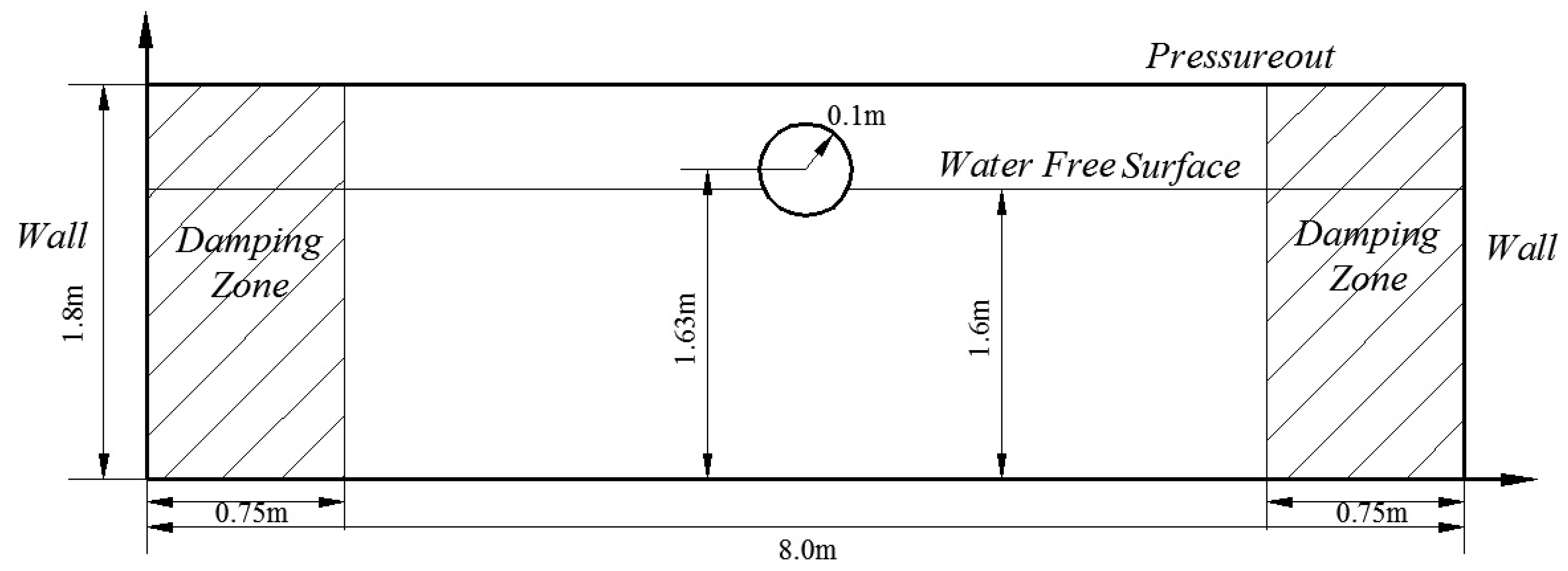
2.2. Numerical Wave Tank

The NWT is 200 m long and 14 m high, and the relative position of the free surface in the numerical domain is 10 m. The schematic of the 2D numerical wave tank is displayed in Figure 2. The sides and bottom of the NWT are defined as the no-slip wall boundary. The pressure-outlet condition is considered to be the top boundary adjacent to the air phase. The grid size Δx is maintained at about 2% of the incident wave length. Furthermore, the grid size Δy around the free surface is refined to be less than 5% but greater than 2% of the incident wave length. The time-step is set as 0.005 s, to guarantee accuracy. A hybrid mesh is created with unstructured mesh near the area of the floating motion, and structured mesh in the other regions. The mesh structures of the NWT are displayed in Figure 2.

The wave-making method applied in this paper is the wave generation source method proposed by Larsen et al. in 1983 [36]. The main idea in this approach is to separate the generation of waves and the absorption of scattered waves, i.e., the incident waves are generated by the application of a distribution of pulsating sources inside the boundary and the scattered waves are absorbed on the boundaries connecting the computational domain to a larger body of water. The schematic of the 2D numerical wave tank is displayed in Figure 3. A finite volume source item set away from the end of the tank is used to generate the desired regular waves. Two damping zones are employed for absorbing waves at two ends of the tank. Accordingly, the continuity Equation (1) can be rewritten as:

$$\{\begin{array}{l}\frac{\partial u}{\partial x}+\frac{\partial v}{\partial y}=0\hspace{0.17em}\hspace{0.17em}\hspace{0.17em}\hspace{0.17em}\hspace{0.17em}\hspace{0.17em}\hspace{0.17em}\hspace{0.17em}\hspace{0.17em}\hspace{0.17em}\hspace{0.17em}\hspace{0.17em}\hspace{0.17em}\hspace{0.17em}\hspace{0.17em}\hspace{0.17em}\hspace{0.17em}\hspace{0.17em}\hspace{0.17em}\hspace{0.17em}\hspace{0.17em}\hspace{0.17em}x\ne x_s\hfill \\ \frac{\partial u}{\partial x}+\frac{\partial v}{\partial y}=q_s\left(y,t\right)\hspace{0.17em}\hspace{0.17em}\hspace{0.17em}\hspace{0.17em}\hspace{0.17em}\hspace{0.17em}\hspace{0.17em}\hspace{0.17em}\hspace{0.17em}\hspace{0.17em}\hspace{0.17em}\hspace{0.17em}\hspace{0.17em}x=x_s\hfill \end{array}$$

(5)

where u, v are the flow velocity components in the x and y direction, respectively.; q_s(y, t) is the wave making intensity, defined as q_s(y, t) = 2w(y, t)/dx, where dx is the cell width of the source volume location. The term w(y, t) is defined as [37]:

$$w(y,t)=\frac{4X_0\omega \sinh \left(k_{w}d\right)·\cosh \left(k_w\right(y+d\left)\right)}{\left(\sinh \right(2k_{w}d)+2k_{w}d)}\cos k_w{x}_s-\omega t$$

(6)

where X₀ is a self-defined constant related to the wave height H and generally needs to be calculated by trial; ω is the circular frequency. Here, k_w and d represent the wave number and water depth, respectively.

In addition, the momentum governing Equation (2), ignoring the Reynolds stress, can be rewritten as:

$$\frac{\partial u}{\partial t}+u\frac{\partial u}{\partial x}+v\frac{\partial u}{\partial y}=-\frac{1}{\rho }\frac{\partial p}{\partial x}+v\left[\frac{{\partial }^{2}u}{\partial x^2}+\frac{{\partial }^{2}u}{\partial y^2}\right]+\frac{1}{\rho }uq+\frac{1}{3}v\frac{\partial q}{\partial x}$$

(7)

$$\frac{\partial v}{\partial t}+u\frac{\partial v}{\partial x}+v\frac{\partial v}{\partial y}=-\frac{1}{\rho }\frac{\partial p}{\partial y}+v\left[\frac{{\partial }^{2}v}{\partial x^2}+\frac{{\partial }^{2}v}{\partial y^2}\right]+\frac{1}{\rho }vq+\frac{1}{3}v\frac{\partial q}{\partial y}-g$$

(8)

An additional source item is added to the momentum governing equations for absorbing an incident wave and guaranteeing no wave reflections. The momentum equations in the damping zones can be written as:

$$\frac{\partial u}{\partial t}+u\frac{\partial u}{\partial x}+v\frac{\partial u}{\partial y}=-\frac{1}{\rho }\frac{\partial p}{\partial x}+v\left[\frac{{\partial }^{2}u}{\partial x^2}+\frac{{\partial }^{2}u}{\partial y^2}\right]-b\left(x\right)\cdot u$$

(9)

$$\frac{\partial v}{\partial t}+u\frac{\partial v}{\partial x}+v\frac{\partial v}{\partial y}=-\frac{1}{\rho }\frac{\partial p}{\partial y}-g+v\left[\frac{{\partial }^{2}v}{\partial x^2}+\frac{{\partial }^{2}v}{\partial y^2}\right]-b\left(x\right)\cdot v$$

(10)

where b(x) is defined as the damping ratio function related to the position on the x-axis, which increases linearly from the end wall to the other boundary of the damping zone.

2.3. Heaving Motion of Buoy

The buoy movement has been constrained to one degree of freedom (DOF) heave motion in the y-direction. This means that the buoy only make the translation motion along the y axis, which is then governed by the resultant force in the y-direction from all static and dynamic components. The velocity at time t is calculated using an explicit Euler formula as:

$$v_t=v_{t-\Delta t}+\left(F_y/m\right)\cdot \Delta t$$

(11)

where F_y is the resultant force in the y-direction, m is the mass of the buoy, and Δt is the time step. The motion of the buoy is specified as a particular dynamic zone by using the translation velocities calculated at every time step. These velocities are used to update the node positions on the dynamic zone of the solid-body motion.

2.4. Numerical Solutions

The commercial CFD software ANSYS-Fluent 12.0 is used to solve all the above equations numerically. The pressure-implicit with splitting of operators (PISO)–non-iterative time-advancement (NITA) scheme is employed for pressure-velocity coupling in the transit calculations, which can balance the computational accuracy and time cost. Neighbor and skewness corrections are also carried out to improve the calculation efficiency. For spatial discretization, PRESTO! and second order upwind schemes are selected for pressure and momentum items. Furthermore, a first-order implicit scheme is used for temporal discretization.

The air and water in the present NWT are both assumed to be immiscible. The volume of fluid (VOF) model then can be used for free water surface tracking through calculation of the volume fraction of each of the fluids throughout the whole domain. The geometric reconstruction scheme is used to reconstruct the interface between fluids using a piecewise-linear approach. The volume fraction spatial discretization employs a first-order upwind implicit scheme.

The dynamic mesh model is used for rigid body motion of the 2D buoys. Smoothing and remeshing methods are applied in the mesh reconstruction. Non-slip wall conditions are applied to the buoy surface, as with the side and bottom walls of the NWT. A pressure outlet boundary condition is enforced on the top of the tank. The wave generation and absorption are realized through the user defined function (UDF) “DEFINE_SOURCE,” and the buoy motion is controlled by “DEFINE_CG_MOTION” in Fluent.

3. Numerical Model Validation

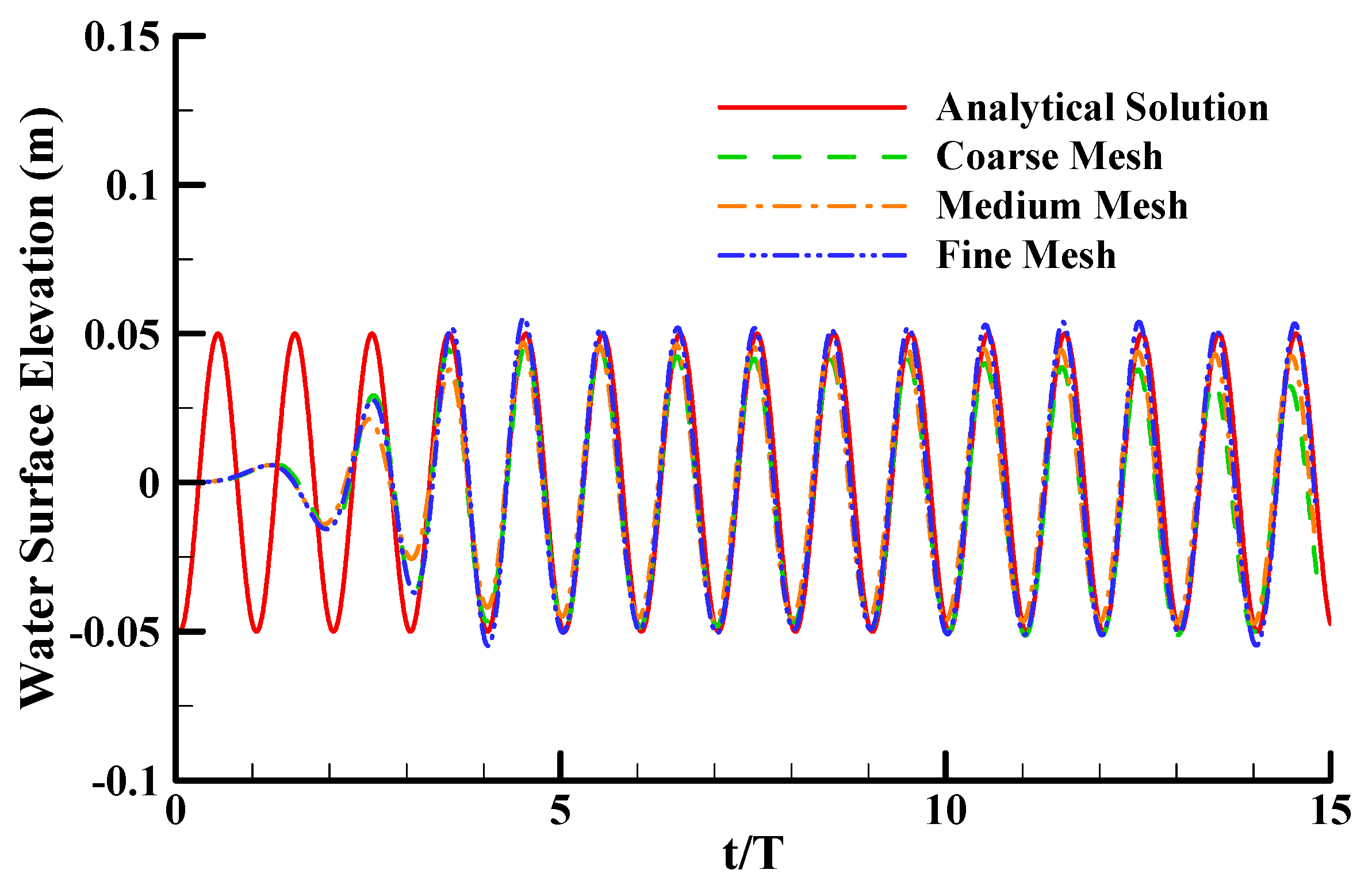
3.1. Regular Wave Generation and Absorbing

As regular waves are utilized in all the case studies of the present paper, they are validated first. Figure 4 illustrates a progressive wave train from left to right. The desired wave height is 0.1 m. The “0” point on the x-axis represents the position two wave-lengths away from the generation source. Here, y/H represents the ratio of water surface elevation to incident wave height. It can be observed that the shape is maintained well during wave propagation. The wave height reduces slightly as the wave moves away from the generation source because of viscous damping effects in the RANS model. This indicates that some redundant values should be considered at the generation source position to guarantee the desired wave height is achieved at the testing position.

For the grid independence study, three grid sizes are tested for comparison: a coarse mesh (10,817 cells), a medium mesh (35,550 cells), and a fine mesh (144,750 cells) As the number of meshes increases, the quality of the mesh also increases significantly with a more appropriate aspect ratio and skew ratio. The calculations were carried out via PC with i7-3770@3.4 GHz CPU and 16 GB RAM.

Grid independence and the effects of the damping zone on wave absorption are illustrated in Figure 5. The figure shows the water surface elevation at a fixed coordinate point three wave-lengths away from the wave generation source. The damping zone is half a wave length away from the fixed recording point. As seen in Figure 5, even after 15 evolutions the wave elevation is still stable and no evident reflection effects are observed. The cross-correlation coefficients of the three grid types are 0.914, 0.884, and 0.618, respectively. The normalized mean square errors (NMSE) are 0.00005, 0.00006, and 0.00017, respectively. This demonstrates that the damping zone shows a good incident wave absorbing capability and can be used for further problem analysis. Under the same redundant value at the wave generating source, medium and coarse meshes both show significant wave height reduction. On the other hand, the numerical results for fine mesh agree well with the analytical solutions.

Mesh numbers and corresponding computing times are shown in

Table 1. Mesh number and corresponding computing time costs.

Mesh Resolution	Coarse Mesh	Medium Mesh	Fine Mesh
Number of Grids	10,817	35,550	144,750
Computation Time	110 min	120 min	580 min

. Although the number of the medium mesh is over three times greater than that of the coarse mesh, its computing time is only 9% higher. Furthermore, the fine mesh, with over 13 times the number of the coarse mesh, takes more than 5 times as much computing time. Taking all the comparisons into account, the medium mesh can effectively predict the performance with an acceptable accuracy and time cost. Hence, the numerical model established in the present work can be considered sufficiently reliable for the following study.

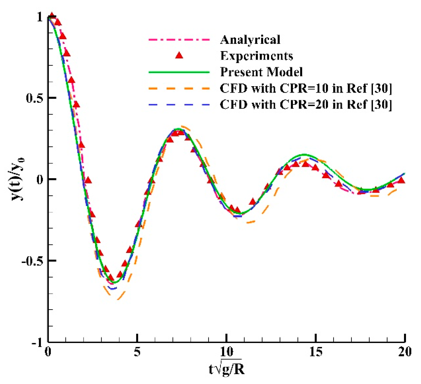
3.2. Free Decay of a Heaving Circular Cylinder

To validate the capability of the present numerical model for the heaving motion of floaters, the free decay problem of a heaving circular cylinder is calculated and compared with the analytical, experimental, and other numerical results. The 2D computation domain of this case is shown in Figure 6. A solid circular cylinder is floating in the still water tank. The radius of the cylinder is 0.1 m and the water depth is 1.6 m (d/R = 16). The length of the still water tank is 8.0 m and the left-side wall is 4.0 m away from the center of the cylinder. The center of gravity of the cylinder is set to be 0.03 m higher than the free water surface level. Two damping zone are considered at two sides to avoid any free surface wave reflection. As the calculation is initialized, the cylinder begins to oscillate in a heaving motion until the cylinder and the water return to their equilibrium state at rest [38].

The numerical heaving motion of the cylinder center versus the dimensionless time $t\sqrt{g/R}$ is compared with other results in Figure 7. All five curves show a similar trend to a harmonic heave oscillation with damping amplitude. CPR represents the number of cells per cylinder radius [38]. The present numerical results show better performance in fitting the experimental curve than the CFD results with CPR = 10 in the reference. Except for the slight overestimation of the third oscillation peak at CPR = 15, the numerical prediction in this paper agrees well with the analytical and experimental data, similar to the CFD model with CPR = 20. The comparison has validated the model capability to predict the transient passive heave motion of the floating body around the free water surface.

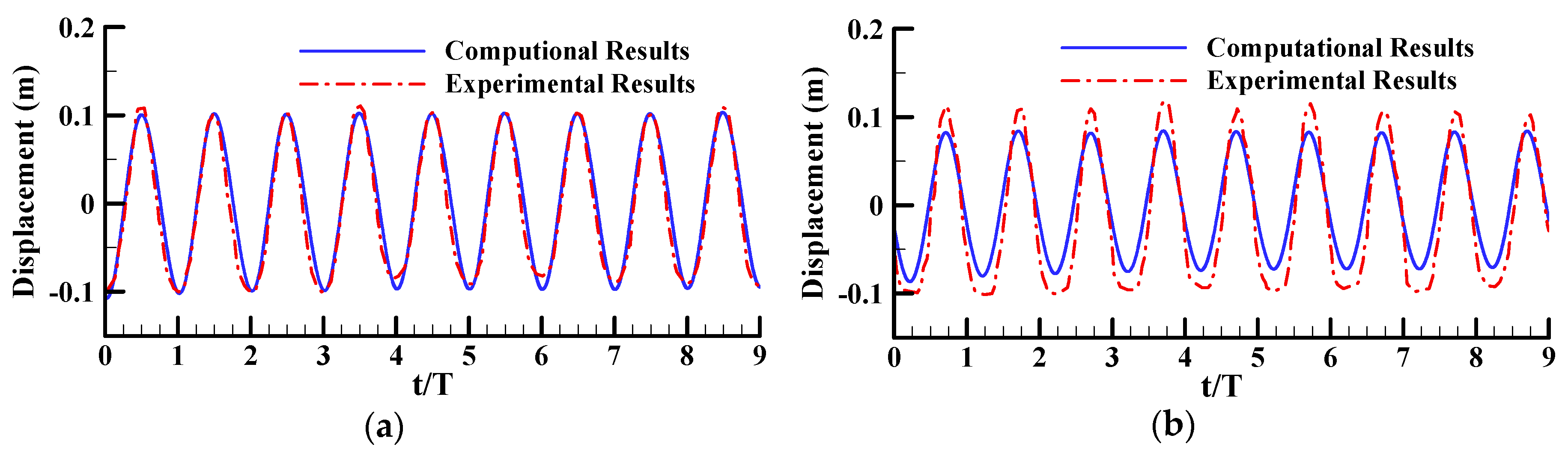
3.3. Heave Oscillation of Floating Buoy Under Wave Excitation

An experimental test of the heave oscillation of a floating buoy under wave excitation is used here to validate the RANS model further. Snapshots of the experiment are shown in Figure 8. Meeting the gravity similarity criterion, the model test length scale is selected as λ_l = 4. Four buoys are installed on the supporting frame in the array, and can only move in translation in one DOF along the guide rod. The buoy shape can be divided into two parts: the upper circular cylinder, and lower cone. The bottom radius is 0.8 m and the total height of the buoy is 0.33 m. The weight of the buoy is 35 kg. The water depth is 1.0 m. Other experiment details can be referred to in previous work [39]. The deployment of the buoy array is simplified in the 2D numerical model and only two buoys are employed in NWT.

A typical wave condition was applied for model validation: wave height H = 0.2 m and wave period T = 2.0 s. The buoys heave freely under the incident wave excitation without any damping or PTO effects. The time histories of translational motions of the buoys’ center in the y-direction are compared between the experimental and numerical results, as shown in Figure 9. The cross-correlation coefficients between the numerical values and the experimental results is greater than 0.939. Although the numerical model is two dimensional, the computational results of heaving motions of the front buoy agree perfectly with the experimental data. For the rear buoy in Figure 9b, the mean peak-to-valley amplitude value of the numerical predictions is about 19% smaller than that of the experimental results. This underestimation may come from the partial lack of wave diffraction and refraction in the 2D model. There is not as much wave energy passing the front buoy to drive the rear one in the numerical model. The validation results indicate that the present model is capable of investigating the hydrodynamic performance of a single buoy. On the other hand, the 3D model is recommended to be considered for the floating buoy array study instead of a 2D model.

4. Results and Discussion

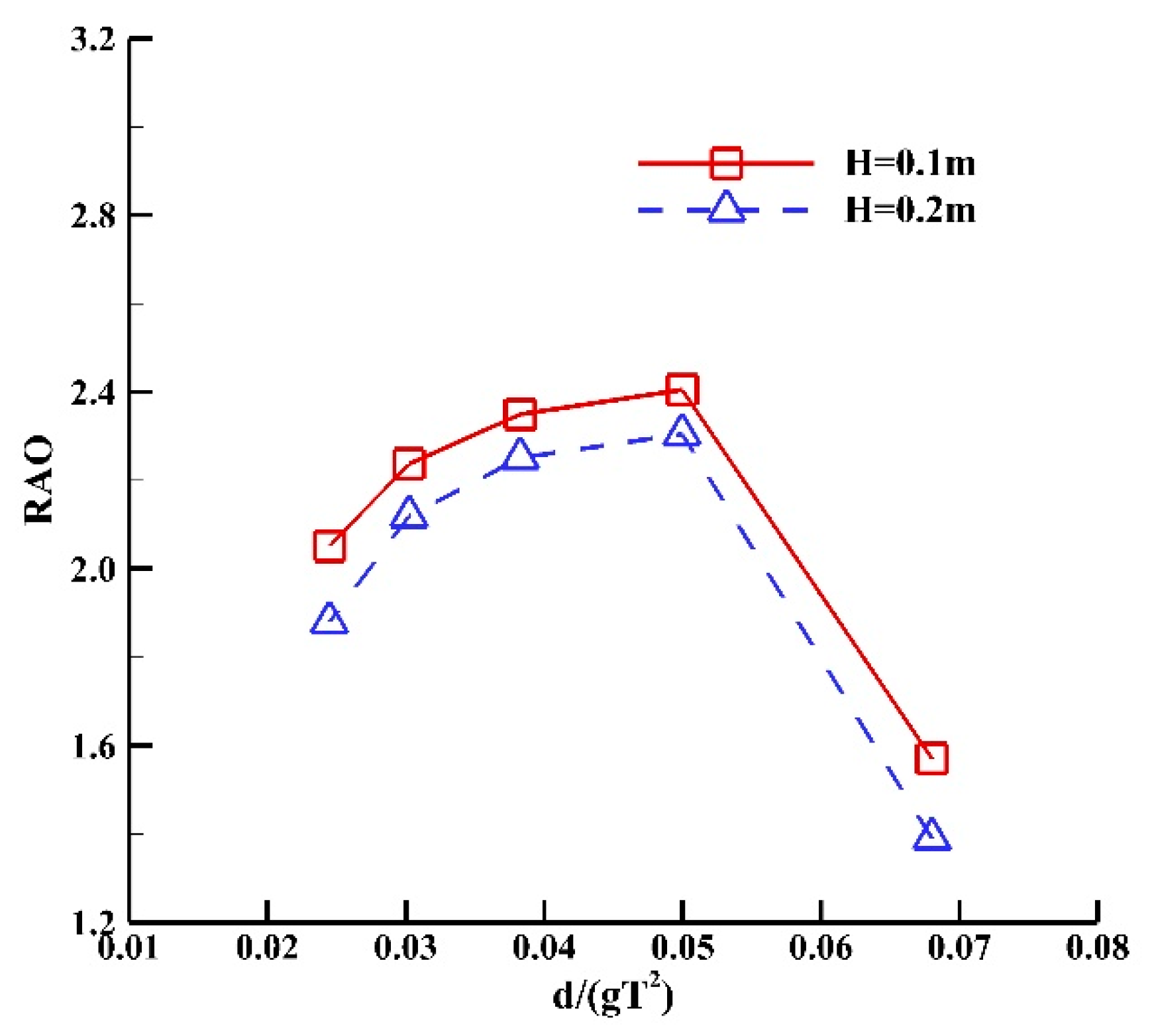
4.1. Effects of Incident Wave Conditions

A 2D square floating body is employed as the typical buoy first. The side length l is 50 cm and the weight of the buoy is 125 kg. Exactly half of the buoy is submerged in the static water. The incident wave conditions include the wave height H = 0.1 m and T = 1.75 s. The water depth is 1.5 m and incident waves come from the left side of the buoy. The buoy motion is restricted to the vertical direction and one DOF. The heave of the buoy and its surrounding flow field characteristics in a wave cycle are illustrated in Figure 10.

In the first half-cycle, the ascending buoy is pushed by the totally upward motion of the water body. A small vortex can be observed at the front edge of the buoy and a relatively low-velocity area is located around the back of the buoy in Figure 10a. As the buoy reaches the peak point in Figure 10b, high-velocity water moves downward from the front submerged corner. By contrast, the high-speed water flows upward past the back corner. As the buoy descends, the overall direction of water flow is from left to right. Because of the shedding effects of the buoy, an obvious separation and vortex, especially at the back corner, can be found in Figure 10c,d.

In the second half-cycle, except for the backward vortex, the water body begins to move downward as the buoy descends, shown in Figure 10e. At the valley point, two vortexes can be found at two underwater corners. During the ascending process, the backward vortex moves to the bottom of the buoy because of the change in direction of water flow. More vortexes can be observed around the buoy when the water flow moves upward. The vortexes are generated around the buoy because of flow separations caused by the sharp corners. These vortexes also cause energy loss during the wave and buoy interactions, and subsequently reduce the energy capture of the floating buoy. A streamlined design of the buoy bottom can significantly reduce the flow separations and improve energy conversion.

Furthermore, the phase relationship between the velocity, displacement of the buoy, and resultant force on the buoy automatically recorded in the numerical model is shown in Figure 11. All testing conditions are the same as in Figure 10. The upward direction is defined as positive along the vertical axis. All three time history curves show sinusoidal shapes under regular wave excitation. The velocity curve has a T/4 phase lag compared to the resultant force on the buoy. A T/4 phase difference can also be observed between the velocity and vertical displacement. These phase differences fit the ideal relationship between forces, velocities, and displacements of a rigid body with one-DOF translation.

The effects of wave conditions on hydrodynamic performance of the buoy are shown in Figure 12. Two wave heights (H = 0.1 m and 0.2 m) and five periods (T = 1.5 s, 1.75 s, 2.0 s, 2.25 s, and 2.5 s, and the corresponding dimensionless frequency d/gT² = 0.073, 0.053, 0.041, 0.032, and 0.026) are selected as the typical wave conditions. A response amplitude operator (RAO) is used to represent the hydrodynamic performance of the buoy. The curves for the two wave heights show the same variation trend and the RAO peaks at around T = 1.75 s. The values of this ratio under H = 0.1 m are all over 2.4, which indicates that the buoy motion is greater than the extent of water surface elevation. Furthermore, the overall performance of H = 0.1 m is on average 7.3% higher than H = 0.2 m. The numerical results demonstrate that the buoy has a matched wave period and height. For the engineering design, it is strongly recommended to carry out this preliminary investigation to look for a suitable buoy size that can match the local wave conditions and amplify the resonant effects for a better hydrodynamic performance and wave energy conversion.

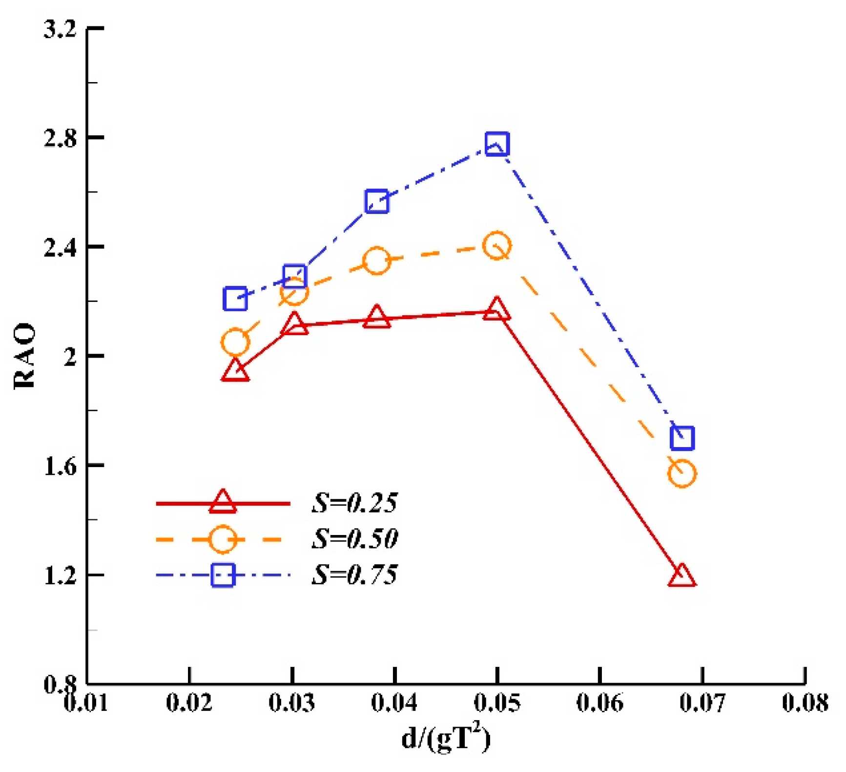
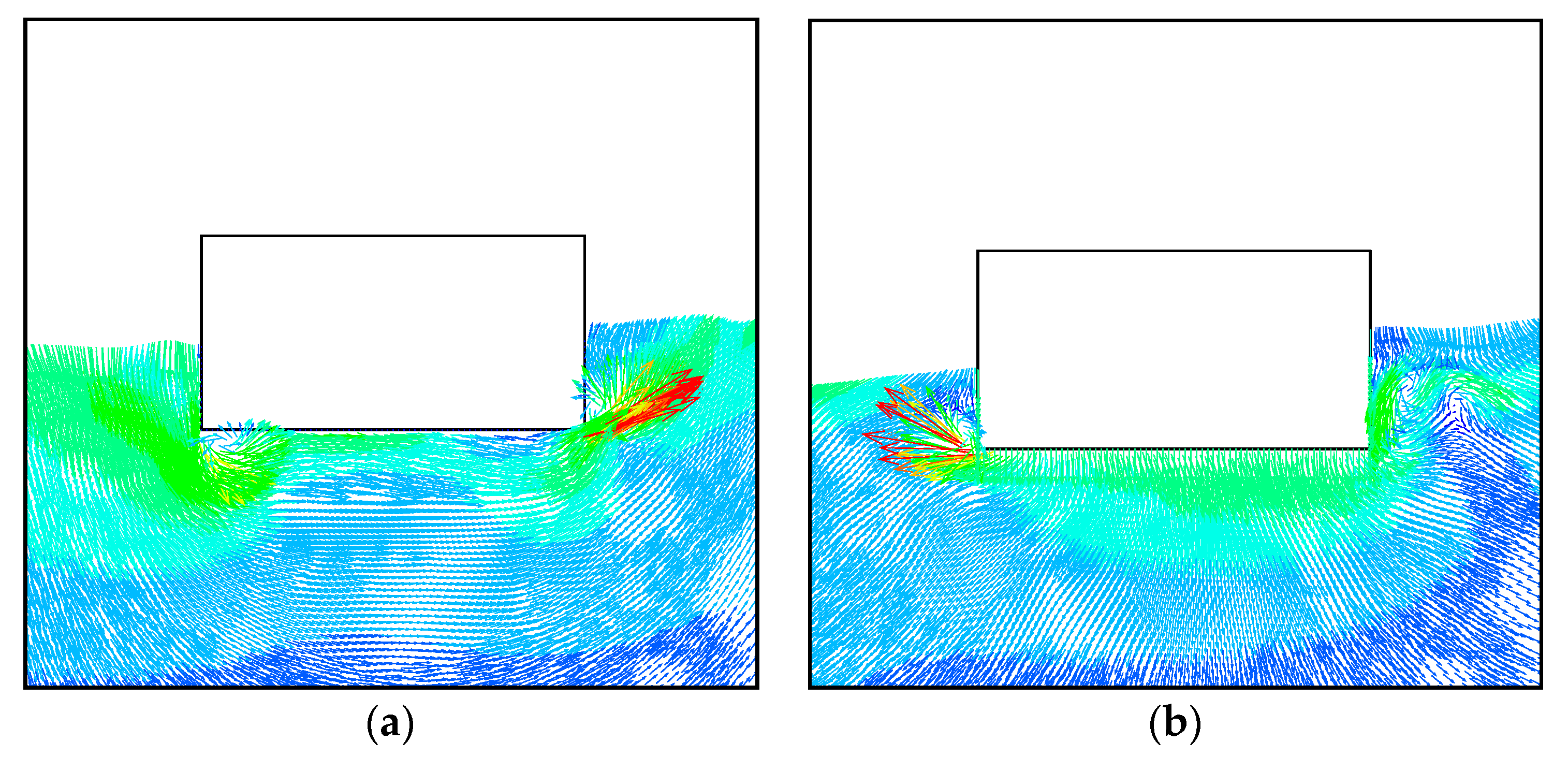
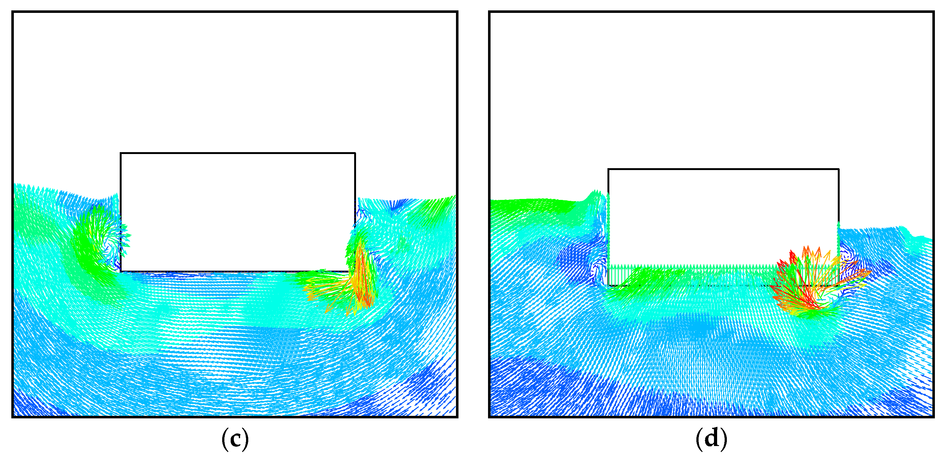
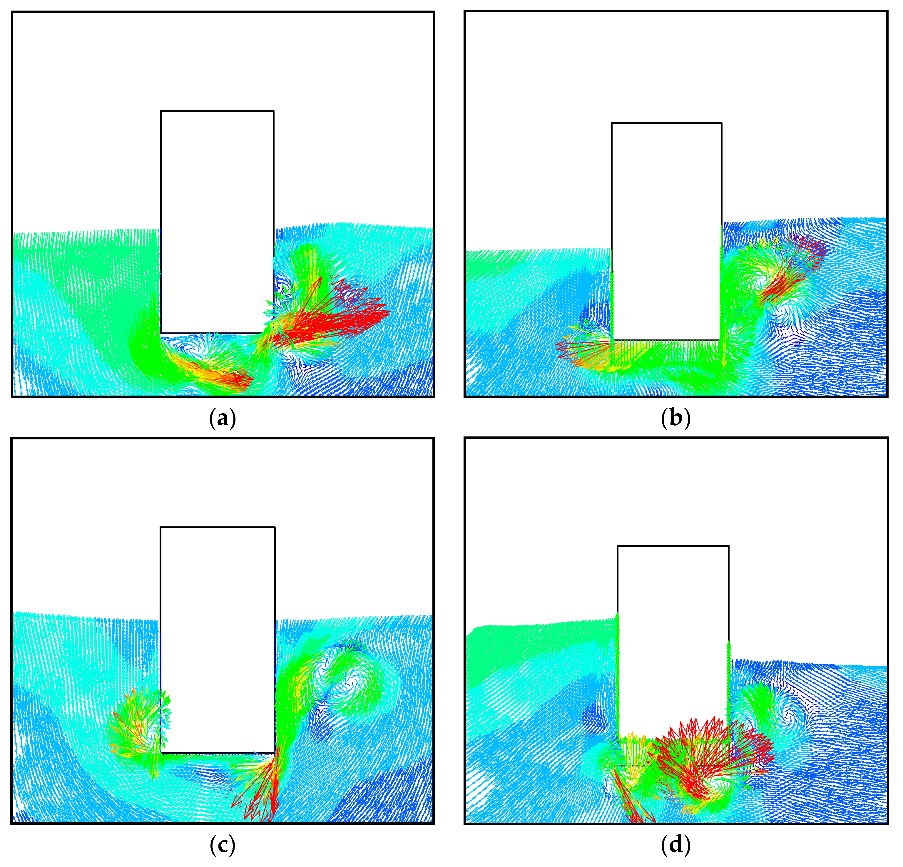
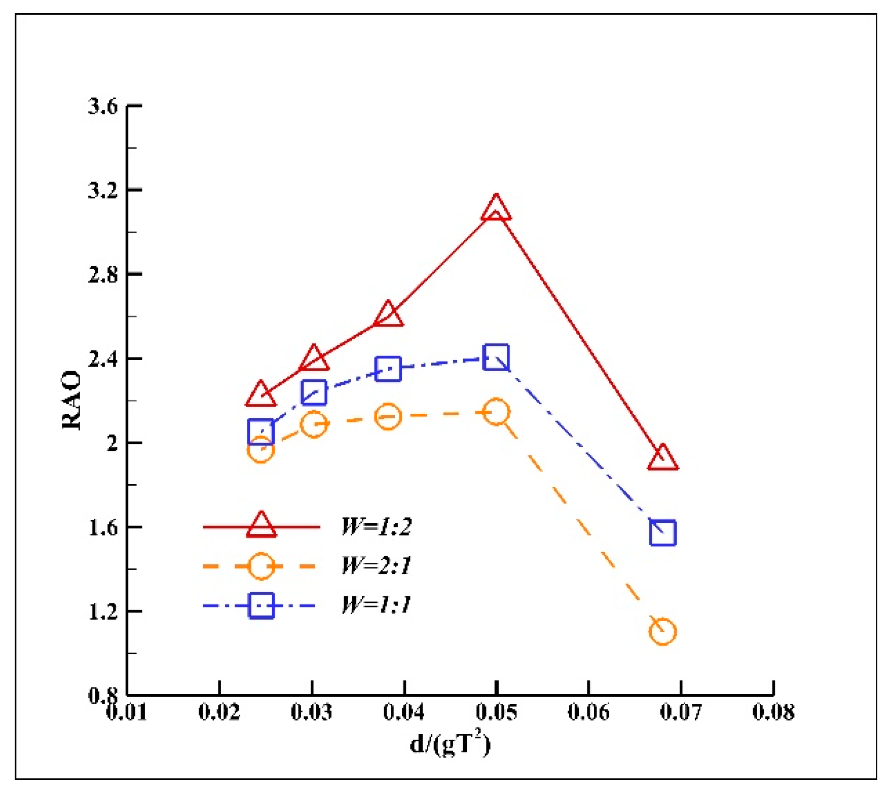
4.2. Effects of Buoy Submerged Depth

Submerged depth is an important factor, which is regarded to have a significant effect on the hydrodynamic performance of the buoy. A square buoy with 50 cm × 50 cm side length is also used here. Two more submerged depths, which could be caused by change in density, are employed. The variation is represented by the ratio S, defined as S = s/l, where s is the submerged depth of the buoy in still water, and this variable is closely related to the mass of the breakwater. When the float mass is 62.5 kg, 125 kg, or 187.5 kg, the corresponding S is 0.25, 0.50, or 0.75, respectively.

Figure 13 illustrates the flow fields around the heaving buoy in a wave cycle (four snapshots) under the wave condition (H = 0.1 m, T = 1.75 s). The submerged depth ratio is S = 0.25. It can be observed that the movement traces of water particles are similar to those in Figure 10 for S = 0.5. Fewer separations and smaller vortexes are found around the underwater corners of the buoy. A less submerged area of small S ratio causes less buoyancy and interaction with incident waves, which works against better hydrodynamic performance for more wave energy conversion.

Figure 14 illustrates the flow fields around the buoy for S = 0.75 in a wave cycle under the same wave conditions as Figure 13. Vectors of significant velocities can be seen in all four snapshots, especially at the two underwater corners. Subsequently, clear vortex flow structures can also be observed. The locations of vortexes depend on the heaving direction of the buoy. During the ascending process, the vortexes mostly locate under the bottom. Accordingly, the vortexes appear at two sides of the buoy during its descent. Wave run-up and overtopping on the tip of the buoy can also be found in Figure 14d. It is obvious that more violent wave-buoy interactions are introduced by the larger submerged depth.

The effects of submerged depth on hydrodynamic performance of the buoy are shown in Figure 15. Three submerged depth ratios are used for comparison. The incident wave height is fixed as 0.1 m. All the three curves have a peak value at the wave period T = 1.75 s, which indicates that submerged depth does not affect the peak period. The ratio S = 0.75 has greater RAO values all over the wave period domain. The peak RAO value for S = 0.75 is up to 2.8.

Furthermore, it is still not certain from the above cases whether it is submerged depth or area that enlarges the heaving ratio RAO. In order to identify which factor has the most significant effect on hydrodynamic performance of the buoy, two more buoys are introduced, which have the same area as the original buoy but different height-to-width ratios (simplified as width ratio W): 0.706 × 0.353 (W = 2:1) and 0.353 × 0.706 (W = 1:2). In addition, the three buoys have the same submerged area, which causes the submerged depths to be 0.353 m (W = 2:1), 0.25 m (W = 1:1) and 0.177 m (W = 1:2).

Figure 16 illustrates the flow fields around the buoy for W = 1:2 in a wave cycle under the wave condition (H = 0.1 m, T = 1.75 s). The movement trend of water particles and location and timing of vortex appearance in this case are similar to those illustrated in Figure 13. Larger flow vectors can also be found at different underwater corners. The flow structure characteristics for W = 2:1 in Figure 17 are also similar to the buoy with greater submerged depth in Figure 14. No wave run-up or overtopping were observed because of the larger height of this slim buoy. At the peak and valley points, it can also be seen that the vortexes are shed further away from the buoy.

The effects of the width ratio on the heaving motion of the buoy are shown in Figure 18. Generally, the slim buoy (W = 2:1) shows better performance than the square buoy across the wave period domain. By contrast, the flat buoy (W = 1:2) has less heaving motion compared to the square buoy. At T = 1.5 s, all three buoys have their smallest value of RAO, all of which are less than 2.0. Similar to other cases, the peak values of RAO for all three buoys are located at T = 1.75 s. The largest peak value of RAO is up to 3.1. The ratios all decrease as the wave period increases. From the above investigations, it can be concluded that the submerged depth is a key factor in the heaving motion of the buoy. More intense fluid structure interactions can be found for a slimmer buoy or larger submerged depth. Greater RAO indicates that a deeply submerged slim buoy has better hydrodynamic performance, and so this is recommended to be utilized for wave energy capture.

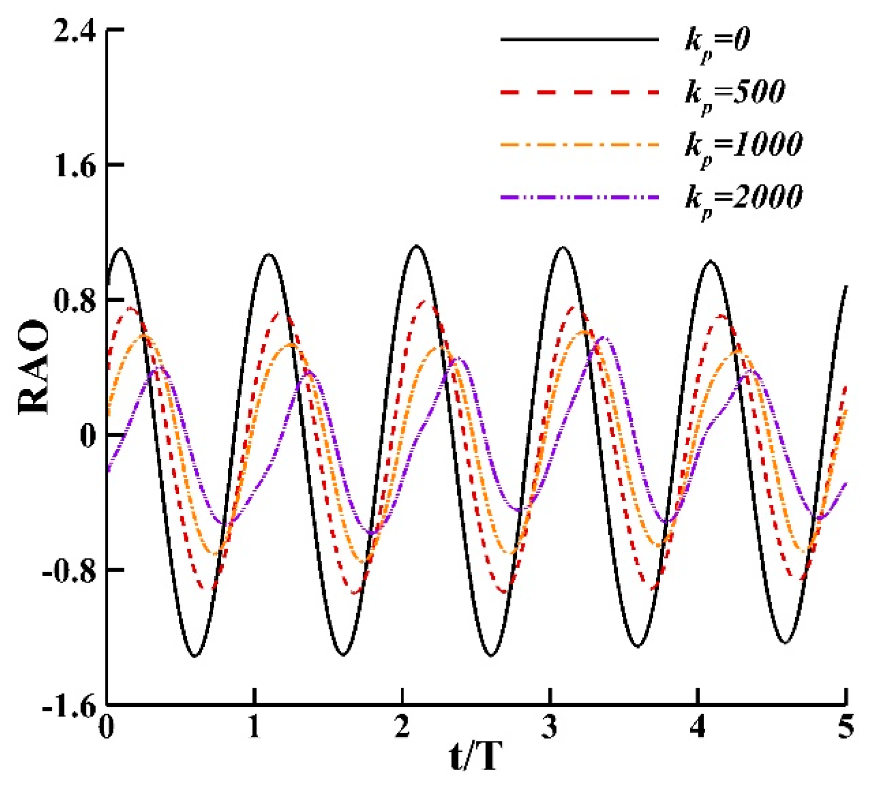
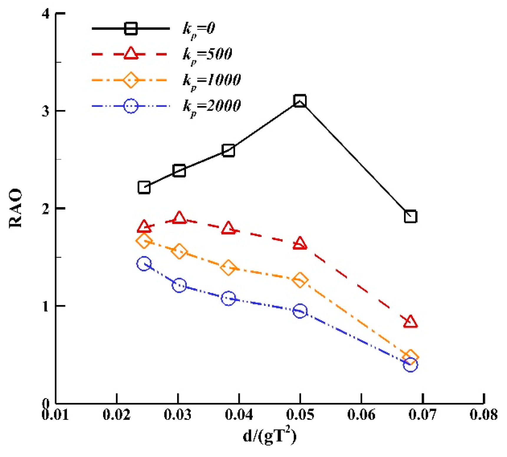
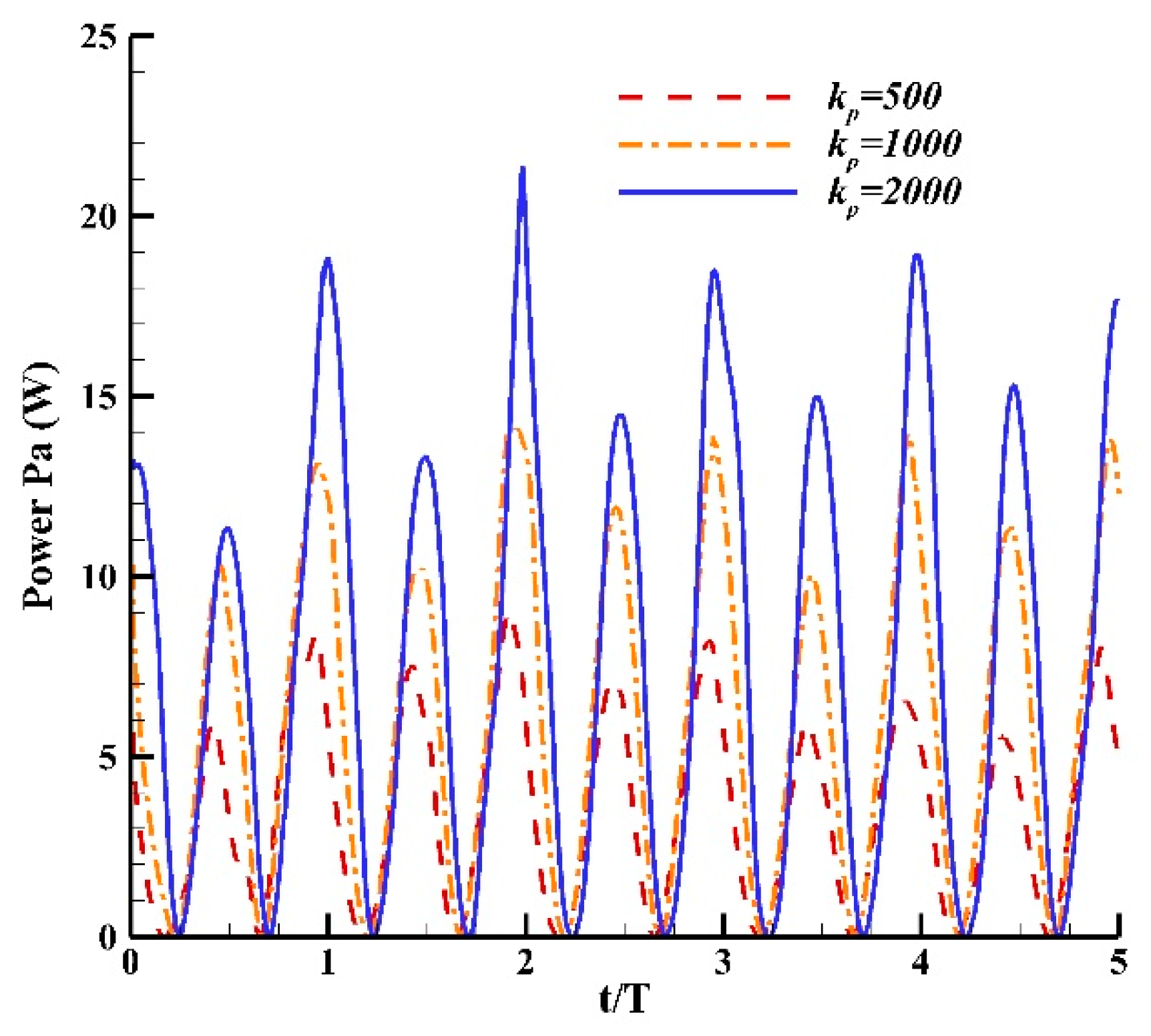
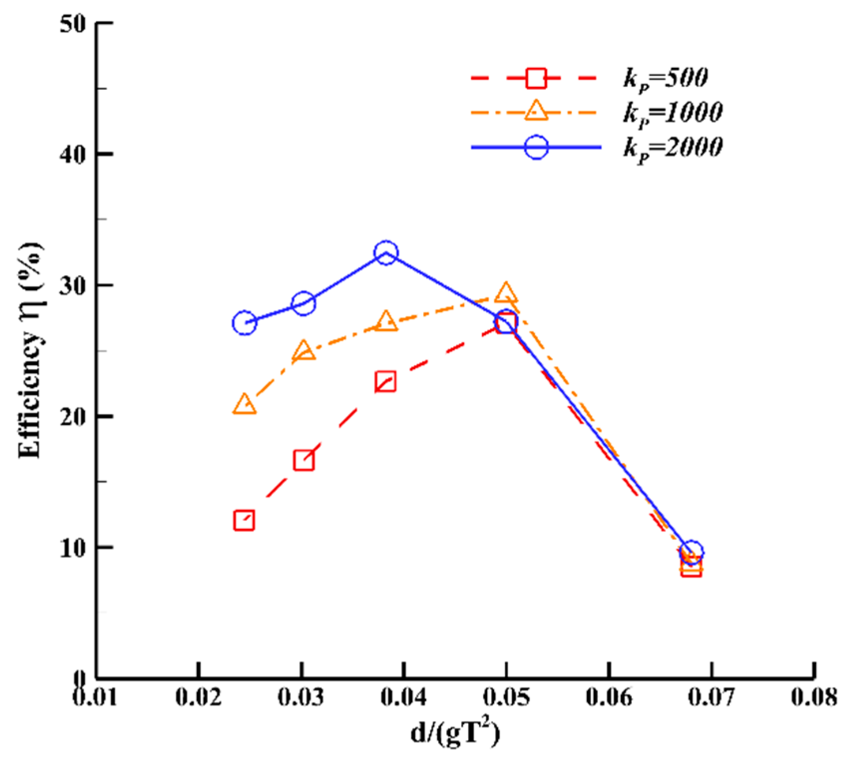
4.3. Effects of PTO Mechanism

A heaving buoy is always connected to hydraulic pressure modules or a rack-and-pinion system to convert mechanical energy into electrical energy. The reaction forces from the above PTO systems are applied on the buoy as external damping forces. Considering the complexity of this force, which is introduced by many nonlinear factors, it is common to model the PTO force as a simple function of the translation velocity of the buoy [14,38,40]. In this study, the PTO damping force is defined as:

$${\overrightarrow{F}}_{PTO}\left(t\right)=-k_p{\overrightarrow{v}}_t\left(t\right)$$

(12)

where k_p is the PTO coefficient, specified as a constant. For dimensional homogeneity, the unit of k_p is N·s/m. In the numerical simulation, the translation velocity of the buoy can be obtained automatically in Fluent. The PTO damping force is then calculated at every time step and imposed on the rigid body of the buoy to derive the new translation acceleration under the resultant force. The velocity is updated to a new value at the next time step to complete a computational cycle.

The time histories of buoy heaving under various PTO damping effects are shown in Figure 19. The heaving amplitude of the buoy becomes smaller as the PTO coefficient k_p increases. The results indicate a decrease in heave motion and an increase in wave energy extraction of the PTO module. Phase shifts and crest-to-trough asymmetry can be observed among the time history curves. The phase lag and asymmetry becomes more apparent as the PTO coefficient k_p increases. In addition, the time history curve with k_p = 2000 shows a quasi-sinusoidal shape, which indicates that more intense PTO effects will cause more instabilities in the device motion pattern.

The effects of the PTO damping coefficient on the hydrodynamic performance of the buoy are shown in Figure 20. Compared to the buoy without PTO effects, the heaving amplitudes of the buoy under three PTO coefficients significantly decrease. In addition, RAO becomes greater as the PTO coefficient decreases over the wave period domain in the numerical simulation. No distinct peaks appear on the heaving amplitude curves of the buoy under PTO effects, which are different from the curve without PTO effects. Except for some individual points, the heaving amplitudes under each PTO coefficient increase gradually as nondimensional frequency decreases.

As PTO effects have been introduced in this study, it is not sufficient to simply use RAO to evaluate the performance of the buoy. The absorbed power and corresponding absorption efficiency will be employed here. The mean absorbed power in a wave cycle can be defined as [37]:

$${\overline{P}}_a=\frac{1}{T}{\displaystyle {\int }_t^{t+T}{P}_a\left(t\right)}dt=\frac{1}{T}{\displaystyle {\int }_t^{t+T}{\overrightarrow{F}}_w\left(t\right)}\cdot {\overrightarrow{v}}_t\left(t\right)dt$$

(13)

where P_a and ${\overline{P}}_a$ are the instantaneous and mean absorbed power, respectively. ${\overrightarrow{F}}_w\left(t\right)$ is the excitation wave force imposed on the buoy, which can be derived from the above equation:

$${\overrightarrow{F}}_a\left(t\right)={\overrightarrow{F}}_w\left(t\right)+{\overrightarrow{F}}_b\left(t\right)+{\overrightarrow{F}}_{PTO}\left(t\right)$$

(14)

where ${\overrightarrow{F}}_b\left(t\right)$ is the buoyancy force, ${\overrightarrow{F}}_a\left(t\right)$ can be calculated as:

$${\overrightarrow{F}}_a\left(t\right)=m\cdot \frac{d{\overline{v}}_t\left(t\right)}{dt}$$

(15)

Hence the wave excitation force imposed on the buoy can be written as:

$${\overrightarrow{F}}_w\left(t\right)=m\cdot \frac{d{\overline{v}}_t\left(t\right)}{dt}-{\overrightarrow{F}}_b\left(t\right)-{\overrightarrow{F}}_{PTO}\left(t\right)$$

(16)

Furthermore, because of the conservative characteristics of buoyancy and inertia forces in the periodic motion of the buoy, Equation (13) can be written as:

$${\overline{P}}_a=\frac{1}{T}{\displaystyle {\int }_t^{t+T}-{\overrightarrow{F}}_{PTO}\left(t\right)}\cdot {\overrightarrow{v}}_t\left(t\right)dt=\frac{1}{T}{\displaystyle {\int }_t^{t+T}k}{\overrightarrow{v}}_t\left(t\right)\cdot {\overrightarrow{v}}_t\left(t\right)dt$$

(17)

The absorption efficiency can be defined as the ratio of the mean absorbed wave power to the incident mean wave power, which is written as [35]:

$$\eta =\frac{{\overline{P}}_a}{{\overline{P}}_w\cdot w}=\frac{\frac{1}{T}{\displaystyle {\int }_t^{t+T}k}{\overrightarrow{v}}_t\left(t\right)\cdot {\overrightarrow{v}}_t\left(t\right)dt}{\frac{1}{8}\rho g{H}^2{c}_g}$$

(18)

where η is the absorption efficiency, the width w is 1 m in the two-dimensional problem, and ρ and g represent the water density and the acceleration due to gravity, respectively; c_g is the wave group velocity.

Figure 21 illustrates the time histories of instantaneous absorbed power of the buoy with three PTO coefficients. The wave conditions are H = 0.1 m and T = 2.5 s. Two zero points can be found in a wave cycle, corresponding to the zero values of translation velocity in one period. High peaks and low peaks occur in a staggered pattern along the x-axis for all three PTO coefficients, depending on whether the buoy moves upward or downward, similar to the phenomena reported in previous work [40]. The corresponding peak values increase with PTO coefficient. The maximum value of the instantaneous absorbed power is found to be 21.4 W for k_p = 2000.

The effects of PTO coefficients on wave power absorption efficiency are shown in Figure 22. The three PTO coefficients show similar effects on absorption efficiency in the small wave period domain (T = 1.5 s and 1.75 s). Absorption efficiency does not change substantially with change in k_p. The absorption efficiencies are around 10% at T = 1.5 s and increase to around 29% at T = 1.75 s, which are also the peaks for k_p = 500 and 1000. As the wave period keeps growing, the efficiencies for k_p = 500 and 1000 begin to decrease. The values for k_p = 500 decrease more rapidly than those for k_p = 1000. On the other hand, the efficiency for k_p = 2000 achieves peak value (34.2%) at T = 2.0 s and then decreases gradually as the wave period increases.

5. Conclusions and Future Works

A 2D numerical wave tank was established based on the RANS equations. All the numerical simulations were conducted using the CFD software ANSYS-Fluent 12.0. The capability of regular wave generation and absorption of the NWT has been validated by the analytical solutions. Two experimental cases of the free decay of a circular cylinder and the heaving motion of a buoy in one DOF were utilized for the numerical simulation using the model in the present paper. Good agreements demonstrate that the numerical model can be employed for heaving buoy analysis.

A 2D rectangular floating body was applied as the typical buoy for wave energy conversion. The numerical results show that the buoy has a peak value of heaving performance at a particular wave condition, including the period and height. It is also suggested that the streamlined underwater shape of the buoy will reduce flow separations, vortex shedding, and energy loss. Submerged depth is a key factor in the heaving performance of the buoy. PTO effects are modeled as a function of the buoy’s translation velocity. Phase shift can be observed when PTO effects are introduced and the RAO decreases as the PTO coefficient increases. High and low peaks occur in a staggered pattern for the instantaneous wave power absorption. For the three PTO coefficients in this paper, a similar effect is shown on the power absorption efficiency in the small wave period domain. A large coefficient (k_p = 2000) can help the buoy to absorb more wave energy. The peak value of the absorption efficiency reaches 34.2%.

These studies prove that the present numerical model can be utilized to provide insight into the hydrodynamics and energy absorption of heaving buoys. Going forward, more investigations will be conducted including a shape parameter study and performance prediction with irregular waves. The 2D numerical wave tank will be extended to a 3D version for more detailed hydrodynamic analysis. Some experiments should be carried out for wave buoy PTO interaction studies and validations. Controlling strategies will be introduced into the numerical model for optimal wave energy absorption and conversion.

References

1. Antonio, F.D.O. Wave energy utilization: A review of the technologies. Renew. Sustain. Energy Rev. 2010, 14, 899–918. [Google Scholar]
2. Hirohisa, T. Sea trial of a heaving buoy wave power absorber. In Proceedings of the 2nd International Symposium on Wave Energy Utilization, Trondheim, Norway, 22–24 June 1982; pp. 403–417. [Google Scholar]
3. Budal, K.; Falnes, J.; Iversen, L.C.; Lillebekken, P.M.; Oltedal, G.; Hals, T.; Hoy, A.S. The Norwegian wave-power buoy project. In Proceedings of the 2nd International Symposium on Wave Energy Utilization, Trondheim, Norway, 22–24 June 1982; pp. 323–344. [Google Scholar]
4. Cleason, L.; Forsberg, J.; Rylander, A.; Sjöström, B.O. Contribution to the theory and experience of energy production and transmission from the buoy-concept. In Proceedings of the 2nd International Symposium on Wave Energy Utilization, Trondheim, Norway, 22–24 June 1982; pp. 345–370. [Google Scholar]
5. Weber, J.; Mouwen, F.; Parish, A.; Robertson, D. WaveBob—Research & development network and tools in the context of systems engineering. In Proceedings of the 8th European Wave Tidal Energy Conference, Uppsala, Sweden, 7–10 September 2009; pp. 416–420. [Google Scholar]
6. Mustapa, M.A.; Yaakob, O.B.; Ahmed, Y.M.; Rheem, C.K.; Koh, K.K.; Adnan, F.A. Wave energy device and breakwater integration: A review. Renew. Sustain. Energy Rev. 2017, 77, 43–58. [Google Scholar] [CrossRef]
7. Garcia-Rosa, P.B.; Cunha, J.P.V.S.; Lizarralde, F.; Estefen, S.F.; Machado, I.R.; Watanabe, E.H. Wave-to-wire model and energy storage analysis of an ocean wave energy hydperbaric converter. IEEE J. Ocean. Eng. 2013, 39, 386–397. [Google Scholar] [CrossRef]
8. Zurkinden, A.S.; Ferri, F.; Beatty, S.; Kofoed, J.P.; Kramer, M.M. Non-linear numerical modelling and experimental testing of a point absorber wave energy converter. Ocean. Eng. 2014, 78, 11–21. [Google Scholar] [CrossRef]
9. Hann, M.; Greaves, D.; Raby, A. Snatch loading of a single taut moored floating wave energy converter due to focussed wave groups. Ocean. Eng. 2015, 96, 258–271. [Google Scholar] [CrossRef] [Green Version]
10. Falnes, J. Ocean Waves and Oscillating Systems: Linear Interactions Including Wave-Energy Extraction; Cambridge University Press: Cambridge, UK, 2002. [Google Scholar]
11. Heikkinen, H.; Lampinen, M.J.; Böling, J. Analytical study of the interaction between waves and cylindrical wave energy converters oscillating in two models. Renew. Energy 2013, 50, 150–160. [Google Scholar] [CrossRef]
12. António, F.D.O. Modelling and control of oscillating-body wave energy converters with hydraulic power take-off and gas accumulator. Ocean. Eng. 2007, 34, 2021–2032. [Google Scholar]
13. António, F.D.O. Phase control through load control of oscillating-body wave energy converters with hydraulic PTO system. Ocean. Eng. 2008, 35, 358–366. [Google Scholar]
14. Ricci, P.; Lopez, J.; Santos, M.; Ruiz-Minguela, P.; Villate, J.L.; Salcedo, F.; Falcão, A.D. Control strategies for a wave energy converter connected to a hydraulic power take-off. IET Renew. Power Gener. 2011, 5, 234–244. [Google Scholar] [CrossRef]
15. Korde, U.A. On a near-optimal control approach for a wave energy converter in irregular waves. Appl. Ocean. Res. 2014, 46, 79–93. [Google Scholar] [CrossRef]
16. Sheng, W.; Alcorn, R.; Lewis, A. On improving wave energy conversion, part I: Optimal and control technologies. Renew. Energy 2015, 75, 922–934. [Google Scholar] [CrossRef]
17. Sheng, W.; Alcorn, R.; Lewis, A. On improving wave energy conversion, part II: Development of latching control technologies. Renew. Energy 2015, 75, 935–944. [Google Scholar] [CrossRef]
18. Evans, D.V.; Jeffrey, D.C.; Salter, S.H.; Taylor, J.R.M. Submerged cylinder wave energy device: theory and experiment. Appl. Ocean. Res. 1979, 1, 3–12. [Google Scholar] [CrossRef]
19. Davis, J.P. Wave energy absorption by the Bristol cylinder-linear and non-linear effects. Inst. Civ. Eng. Proc. 1990, 89, 317–340. [Google Scholar] [CrossRef]
20. Liu, Z.; Cui, Y.; Zhao, H.; Shi, H.; Hyun, B.S. Effects of damping plate and taut-line system on mooring stability of small wave energy convertor. Math. Probl. Eng. 2015, 1–10. [Google Scholar] [CrossRef]
21. Oskamp, J.A.; Özkan-Haller, H.T. Power calculations for a passively tuned point absorber wave energy converter on the Oregon coast. Renew. Energy 2012, 45, 72–77. [Google Scholar] [CrossRef] [Green Version]
22. Harnois, V.; Weller, S.; Johanning, L.; Thies, P.R.; Le Boulluec, M.; Le Roux, D.; Soulé, V.; Ohana, J. Numerical model validation for mooring systems: Method and application for wave energy converters. Renew. Energy 2015, 75, 869–887. [Google Scholar] [CrossRef] [Green Version]
23. Li, Y.; Yu, Y.H. A synthesis of numerical methods for modelling wave energy converter-point absorbers. Renew. Sustain. Energy Rev. 2012, 16, 4352–4364. [Google Scholar] [CrossRef]
24. Agamloh, E.B.; Wallace, A.K.; Von Jouanne, A. Application of fluid–structure interaction simulation of an ocean wave energy extraction device. Renew. Energy 2008, 33, 748–757. [Google Scholar] [CrossRef]
25. Bhinder, M.; Mingham, C.; Causon, D.; Rahmati, M.; Aggidis, G.; Chaplin, R. Numerical and experimental study of a surging point absorber wave energy converter. In Proceedings of the 8th European Wave and Tidal Energy Conference, Uppsala, Sweden, 7–10 September 2009. [Google Scholar]
26. Yu, Y.; Li, Y. A RANS simulation for the heave response of a two-body floating point wave absorber. In Proceedings of the 21st international Offshore (Ocean) and Polar Engineering Conference, Trondheim, Norway, 22–24 June 2011. [Google Scholar]
27. Vicinanza, D.; Dentale, F.; Salerno, D.; Buccino, M. Structural response of Seawave Slot-Cone Generator (SSG) from Random Wave CFD simulations. In Proceedings of the International Offshore and Polar Engineering Conference (ISOPE 2015), Kona, HI, USA, 21–26 June 2015; pp. 985–991. [Google Scholar]
28. Buccino, M.; Dentale, F.; Salerno, D.; Contestabile, P.; Calabrese, M. The Use of CFD in the Analysis of Wave Loadings Acting on Seawave Slot-Cone Generators. Sustainability 2016, 8, 1255. [Google Scholar] [CrossRef]
29. Zhao, X.; Ning, D.; Zhang, C.; Liu, Y.; Kang, H. Analytical study on an oscillating buoy wave energy converter integrated into a fixed box-type breakwater. Math. Probl. Eng. 2017, 2017, 3960401. [Google Scholar] [CrossRef]
30. Zhao, X.; Ning, D.; Zhang, C.; Kang, H. Hydrodynamic investigation of an oscillating buoy wave energy converter integrated into a pile-restrained floating breakwater. Energies 2017, 10, 712. [Google Scholar] [CrossRef]
31. Ning, D.; Zhao, X.; Göteman, M.; Kang, H. Hydrodynamic performance of a pile-restrained WEC-type floating breakwater: An experimental study. Renew. Energy 2016, 95, 531–541. [Google Scholar] [CrossRef]
32. Zhao, X.L.; Ning, D.Z.; Liang, D.F. Experimental investigation on hydrodynamic performance of a breakwater-integrated WEC system. Ocean. Eng. 2019, 171, 25–32. [Google Scholar] [CrossRef]
33. Zhang, H.C.; Xu, D.L.; Liu, C.R.; Wu, Y.S. Wave energy absorption of a wave farm with an array of buoys and flexible runway. Energy 2016, 109, 211–223. [Google Scholar] [CrossRef]
34. Ansys Inc. ANSYS Fluent 12.0 Theory Guide; Ansys Inc.: Canonsburg, PA, USA, 2009. [Google Scholar]
35. Yakhot, V.; Orszag, S.A. Renormalization Group Analysis of Turbulence: I. Basic Theory. J. Sci. Comput. 1986, 1, 1–51. [Google Scholar] [CrossRef]
36. Larsen, J.; Dancy, H. Open boundaries in short wave simulations—A new approach. Coast. Eng. 1983, 7, 285–297. [Google Scholar] [CrossRef]
37. Li, S.Z. Study on 2D Numerical Wave Tank Based on Fluent. Master’s Thesis, Harbin Institute of Technology, Harbin, China, 2006. [Google Scholar]
38. Anbarsooz, M.; Passandideh-Fard, M.; Moghiman, M. Numerical simulation of a submerged cylinder wave energy converter. Renew. Energy 2014, 64, 132–143. [Google Scholar] [CrossRef]
39. Qu, N. Study on Hydrodynamic Performance of Oscillating Buoy WEC Considering Power Take-Off System. Master’s Thesis, Ocean University of China, Qingdao, China, 2014. [Google Scholar]
40. Yu, Y.H.; Li, Y. Reynolds-averaged Navier-Stokes simulation of the heave performance of a two-body floating-point absorber wave energy system. Comput. Fluids 2014, 73, 104–114. [Google Scholar] [CrossRef]
Figure 1. Schematic of heaving-buoy integrated floating breakwater.
Jmse 07 00239 g001
Figure 2. Mesh structures of numerical wave tank (NWT).
Jmse 07 00239 g002
Figure 3. Schematic of Numerical Wave Tank.
Jmse 07 00239 g003
Figure 4. Illustration of a regular progressive wave train.
Jmse 07 00239 g004
Figure 5. Time histories of water surface elevation at a fixed point with different mesh numbers.
Jmse 07 00239 g005
Figure 6. Computational domain of the free decay problem of a circular cylinder.
Jmse 07 00239 g006
Figure 7. Comparison of various results for free decay amplitude variation of a circular cylinder in still water.
Jmse 07 00239 g007
Figure 8. Snapshots of heaving buoys under wave excitation.
Jmse 07 00239 g008
Figure 9. Comparison of time histories of buoy heaving motions: Experimental and numerical results. (a) Front Buoy; (b) Rear Buoy.
Jmse 07 00239 g009
Figure 10. Flow fields around the buoy in a wave cycle (H = 0.1 m, T = 1.75 s). (a) t = T/8; (b) t = 2T/8; (c) t = 3T/8; (d) t = 4T/8; (e) t = 5T/8; (f) t = 6T/8; (g) t = 7T/8; (h) t = 8T/8.
Jmse 07 00239 g010aJmse 07 00239 g010b
Figure 11. Phase relationship among resultant force, velocity, and displacement of the buoy.
Jmse 07 00239 g011
Figure 12. Effects of wave conditions on hydrodynamic performance of the buoy.
Jmse 07 00239 g012
Figure 13. Flow fields around the buoy in a wave cycle (S = 0.25, H = 0.1 m, T = 1.75 s): (a) t = T/4; (b) t = 2T/4; (c) t = 3T/4; (d) t = 4T/4.
Jmse 07 00239 g013aJmse 07 00239 g013b
Figure 14. Flow fields around the buoy in a wave cycle (S = 0.75, H = 0.1 m, T = 1.75 s): (a) t = T/4; (b) t = 2T/4; (c) t = 3T/4; (d) t = 4T/4.
Jmse 07 00239 g014
Figure 15. Effects of submerged depth on hydrodynamic performance of the buoy (H = 0.1 m).
Jmse 07 00239 g015
Figure 16. Flow fields around the buoy in a wave cycle (W = 1:2, H = 0.1 m, T = 1.75 s): (a) t = T/4; (b) t = 2T/4; (c) t = 3T/4; (d) t = 4T/4.
Jmse 07 00239 g016aJmse 07 00239 g016b
Figure 17. Flow fields around the buoy in a wave cycle (W = 2:1, H = 0.1 m, T = 1.75 s): (a) t = T/4; (b) t = 2T/4; (c) t = 3T/4; (d) t = 4T/4.
Jmse 07 00239 g017
Figure 18. Effects of width ratio on hydrodynamic performance of the buoy (H = 0.1 m).
Jmse 07 00239 g018
Figure 19. Time histories of buoy heaving under various PTO damping effects (H = 0.1 m, T = 1.75 s).
Jmse 07 00239 g019
Figure 20. Effects of PTO coefficient on hydrodynamic performance of the buoy (H = 0.1 m).
Jmse 07 00239 g020
Figure 21. Time histories of instantaneous absorbed power of the buoy (H = 0.1 m, T = 2.50 s).
Jmse 07 00239 g021
Figure 22. Effects of PTO coefficient on wave power absorption efficiency (H = 0.1 m).
Jmse 07 00239 g022