Mechanics and Historical Evolution of Sea Level Blowouts in New York Harbor

Abstract

Wind-induced sea level blowouts, measured as negative storm surge or extreme low water (ELW), produce public safety hazards and impose economic costs (e.g., to shipping). In this paper, we use a regional hydrodynamic numerical model to test the effect of historical environmental change and the time scale, direction, and magnitude of wind forcing on negative and positive surge events in the New York Harbor (NYH). Environmental sensitivity experiments show that dredging of shipping channels is an important factor affecting blowouts while changing ice cover and removal of other roughness elements are unimportant in NYH. Continuously measured water level records since 1860 show a trend towards smaller negative surge magnitudes (measured minus predicted water level) but do not show a significant change to ELW magnitudes after removing the sea-level trend. Model results suggest that the smaller negative surges occur in the deeper, dredged modern system due to a reduced tide-surge interaction, primarily through a reduced phase shift in the predicted tide. The sensitivity of surge to wind direction changes spatially with remote wind effects dominating local wind effects near NYH. Convergent coastlines that amplify positive surges also amplify negative surges, a process we term inverse coastal funneling.

1. Introduction

A negative surge, which occurs when the difference between observed water level and predicted astronomical tide is negative, is produced when winds “blow out” the water from a harbor or estuary (hence the name “sea level blowout”). Sea level blowouts have long been tabulated by government agencies (e.g., [1]), and continue to be reported (e.g., by the National Oceanographic and Atmospheric Administration—NOAA), due to the risk of grounding posed to ships. The strong currents associated with negative surge cause erosion and pose a recreational hazard, similar to the much more-often studied positive surge events (which carry the additional hazard of flooding). For example, the drying-out of Tampa Bay during Hurricane Irma caused a safety concern for uninformed people [2]. Significant economic losses are caused by shipping delays [3], and accurate forecasting of blowouts can be important to nuclear power plants, for cooling water intake [4].

The main factors affecting both positive and negative surge are wind, bathymetry, tide, currents and waves (e.g., [5,6]). As with a positive surge, a negative surge is impacted both by “local” wind stress within the harbor and by wind set-down caused by the fetch, wind velocity, duration, and size of the event. Given differences with negative and positive surge events in the temporal evolution of wind stress direction, wave heights, and mean depth, one might posit that the local and coastal response of a system will inherently produce different magnitude extremes. Indeed, assessments of residual water levels after taking out the predicted tide often show a marked asymmetry between positive and negative deviations (e.g., the Newlyn gauge in England; see p. 165 in [5]). Over time, changes to atmospheric forcing or coastal geometry can shift this balance; for example, Raicich [7] studied the trends in positive and negative surges in the Adriatic Sea and showed that the frequency of strong surges decreased over the period of study (1939–2001), while weak and moderate surges did not exhibit any clear trend. This trend was attributed to a weakening of atmospheric forcing over the period. For stations around the United Kingdom where tide surge interaction was insignificant, Pugh and Vassie [8] showed that, using the independent probability distributions for surge and tide, the probability of occurrence of sea level extremes was comparable to those obtained by the traditional method of fitting probability distributions to annual maximum and minimum sea levels.

In the New York-New Jersey Harbor (NYH), positive storm surge and storm tide (surge plus astronomical tide) magnitudes have significantly outpaced sea-level level rise since the mid-19th century [9], and channel deepening has reduced tidal current amplitudes, altered exchange flows, and increased tide magnitudes (e.g., [10,11]). Recent studies by Orton et al. [12] and Familikhalili and Talke [13] showed that positive surge magnitudes can be extremely sensitive to depth changes, to an extent related to percent depth change but also to the magnitude of tide change. Since tidal amplitude changes within NYH are slight (~5%), it remains unclear to what extent a doubling of channel depths in the harbor has influenced surge magnitudes in New York City. Other changes in environmental factors, such as changing ice-cover [14], altered connectivity between sub-embayments, or altered storm tracks (for example caused by NAO; see e.g., [15]) have occurred, and may be important. A novel approach to study long-term changes and local versus far field effects may be to study whether negative surges have changed over time, since the relative change in water depth during a negative surge is larger than for positive surge.

In this paper, the main goals are (1) to explore the evolution of blowouts (both negative surges and extreme low water (ELW) events) in NYH and the Hudson estuary from 1860 to the present, (2) gain an improved understanding of the fundamental mechanics of blowouts in NYH, and (3) evaluate possible reasons for historical changes to blowouts. In Section 2, we begin with a background overview of the region’s geography, as well as several factors like dredging of shipping channels, the ice formation and presence of reefs in the Hudson and the East River, that may have influenced the historical evolution of blowouts. In Section 3, we present the modeling techniques, experimentation approaches and data analysis methods used to understand the mechanics and evolution of blowouts. The results are shown and discussed in Section 4. The paper closes in Section 5 with a summary and conclusions.

2. Background

New York-New Jersey Harbor (NYH) lies at the confluence of the Hudson River Estuary, the East River and New York Bight. NYH includes the Port of New York and New Jersey, Port Newark and comprises multiple sub-embayments including Newark Bay, Raritan Bay and Upper New York Bay (Figure 1). The Harbor opens into the Atlantic Ocean (through the apex of New York Bight) to the southeast and the Long Island Sound to the northeast. The Journal of Commerce recorded cargo valued more than $200 billion entering NYH [16,17]. In this section, we describe the many historical changes to the harbor as a context for understanding observed historical changes in blowouts.

2.1. Shipping Channel Bathymetry

Ambrose Channel is the entrance channel to lower NYH and is located between Sandy Hook, New Jersey (NJ), and the Rockaway peninsula, New York (shown in Figure 1b as a deep channel). It stretches from the apex of the New York Bight to the Verrazano Bridge. This channel is routinely dredged to the depth required by the incoming vessels. The depth and width of the channel has evolved with the growth of ship sizes since the dredging began in the late 1800s [11]. Channels with controlling depths (minima) of 6 to 7.6 m existed in the 1800s [18,19], and by 1914, the Ambrose channel was created at a depth of 12.2 m [20,21]; however, this depth and width were further modified several times through the 20th century. Most recently, in the past decade, the channel was deepened further to 15.8 m [22]. Because deepening a shipping channel can significantly change the physical processes [10], we will examine the sensitivity of surges to deepening of the Ambrose channel.

2.2. Reefs

During the 1800s, the harbor contained many “reefs”, or rock formations, which produced an impediment to flow and shipping. The presence of reefs could have altered the quantity of tidal transport through the relatively narrow East River and affect the mechanics of blowouts in NYH. Major impediments for tidal flow were large reefs at Hell Gate, located at the junction of the Harlem River and the East River tidal straits (labeled as “East River wall” in Figure 1a). In the late 1800s, the reefs were dynamited by various agencies including United States Army Corps of Engineers (USACE). In this paper, we simulate pre-removal conditions to emulate an extreme scenario of reefs (by a wall), to test if the removal of this impediment will affect surge magnitudes in NYH.

2.3. Ice Formation on the Hudson

Historical data show that more than 90% of the blowout events occurred during the cool season from December to March when extratropical cyclones (e.g., nor’easters) occur and there are no tropical cyclones. This time period also often correlates with reduced river flow, due to the formation of ice on the Hudson. While river flow typically has a negligible effect on NYH water levels [23], the formation of ice produces measurable effects on tides [14] and alters the surface boundary condition, and therefore, may affect the local component of negative surge. In particular, measurements suggest that ice formation and duration was much longer in the 19th century, leading to large freshets during spring thaw [1,11]; by contrast, winter flows are measurably larger today [11]. The formation of ice takes many forms such as brash ice, drift ice, fast ice, floe formations, or ice jams to name a few. Of these formations, shore-fast ice and ice jams are typically observed in the Hudson River north of Piermont, with drift ice being observed in southern areas of the Hudson River near Manhattan [24]. By “shore-fast” ice, we are referring to ice that is horizontally but not vertically stationary, as the tide moves the ice and it is not actually attached to the shoreline. Ice reports from the United States Coast Guard (USCG) suggest that ice jams historically occurred in the Hudson River near West Point and Albany. The effect of ice friction on tidal ranges has been studied by Georgas [14] who showed that the friction from shore-fast ice can affect the tidal ranges and currents. Ice formation in an extreme case such as ice jams can block the flow of the river to the south, causing flooding upstream, and lowering the water levels downstream of the ice jam. Due to their potentially large influence on water levels in the Hudson River, we also evaluate their possible role in negative surges in NYH.

3. Methodology

Our analysis of sea level blowouts consists of four parts, with methods summarized below—(1) historical tide gauge data analysis and extreme value analysis, (2) historical meteorological data analysis, (3) modeling of recent blowout events to evaluate modeling accuracy, and (4) model-based environmental sensitivity experiments to study the mechanics and sensitivities of blowouts in the NYH region.

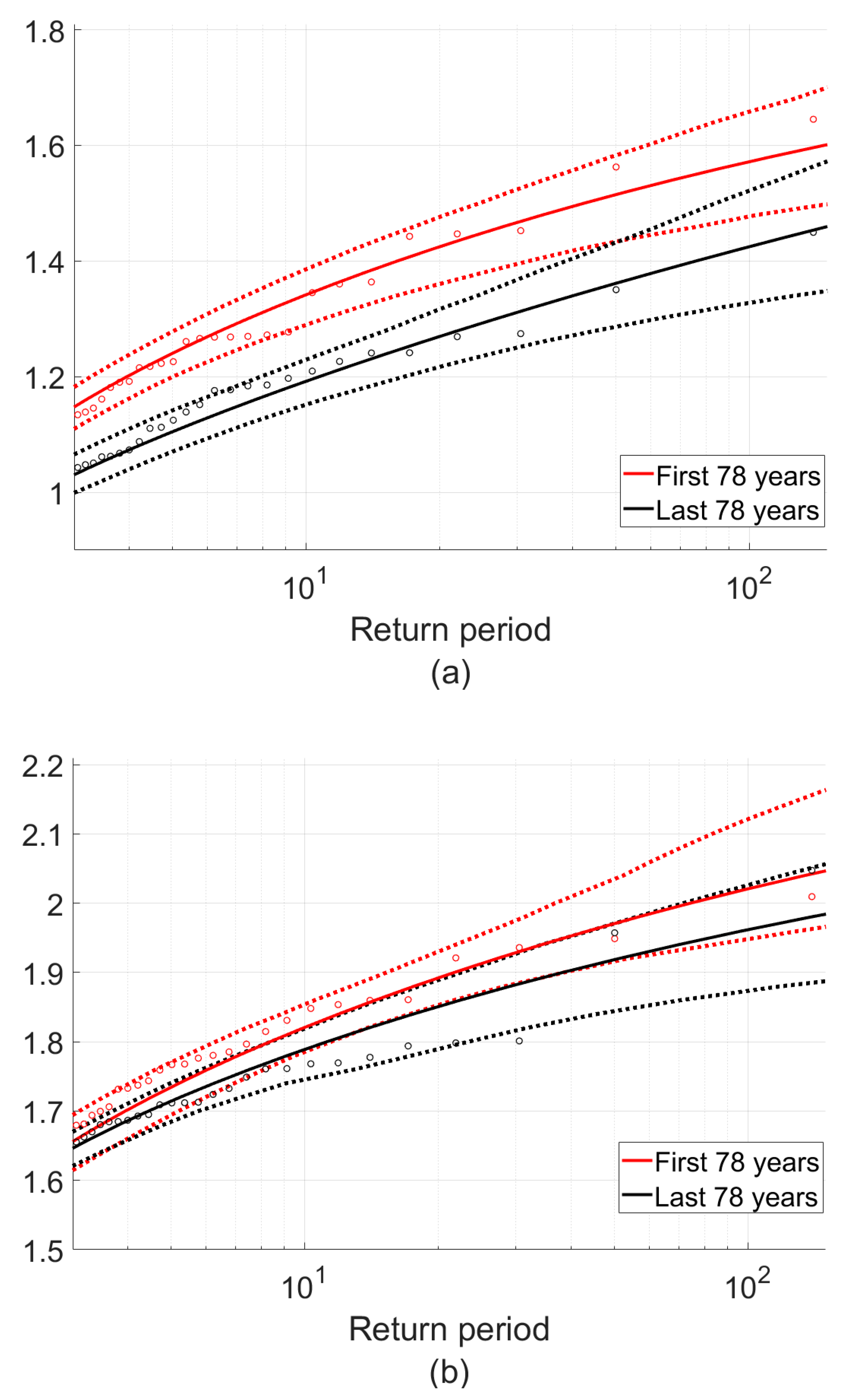
3.1. Historical Data Compilation and Extreme Value Analysis

In this study, we assemble and evaluate historical time series of annual minimum storm surge (negative surges) and annual minimum storm tide (total water levels, with annual sea-level removed), with latter representing ELWs. Tide gauge records from 1860 to 2015 are assembled from four stations in NYH—The Battery, Governors Island, Sandy Hook and Fort Hamilton, following the archival research and methods described in Talke et al. [9]. The compiled raw data is a collection of hourly water level data from the mentioned tide gauges for different periods, depending on availability of the data. For each year and station, we: (1) perform standard least squares harmonic analysis [25,26] using the available hourly water level data, (2) predict a tide time series and subtract it from the total water level time series to obtain storm surge data, (3) compute and subtract the annual mean sea level from the total water level and surge time series, and (4) compute the annual minima of storm surge (AMnSS) and storm tide (AMnST). This procedure was performed to all the years with at least 95% of the data in the winter months (Nov-Mar). The values from the Sandy Hook gauge were corrected for the distance from The Battery by applying a bias correction of −0.023 m for AMnST and 0.027 m for AMnSS, obtained from the median difference in AMST or AMnSS values between Sandy Hook and The Battery from 1911 to 2013 (91% coincident values, σ = 0.11 m for AMnST and AMnSS).

Two extreme examples of NYH blowout events are shown in Figure 2. Figure 2a shows the water level in NYH in a 1978 blowout event that has the most negative water level in the compiled data set. The water level plunges to a low of −2.05 m with a negative surge of −1.22 m (relative to mean sea level). Figure 2b shows a minimum water level of −1.74 m in NYH in an 1862 blowout event that had strongest measured negative surge of −1.64 m (since 1860).

Statistical extreme value analysis is performed on the historical data to evaluate the long-term change, with the 154 years of data divided into two periods to qualitatively represent ‘past’ and ‘present’ versions of the harbor. The corresponding data of annual water level (AMnST) and surge (AMnSS) minima are then fit with generalized extreme value (GEV) distributions, with 95% bootstrapped confidence intervals and the water levels and corresponding return periods are compared for the two periods (Section 4.1).

3.2. Meteorological Conditions during Past Blowouts

We investigate the meteorological conditions leading to blowouts by looking at the top 25 negative surge events from 1979–2014 in two ways by—(1) creating regional composite (average across events) 10 m wind velocity and sea level pressure data using meteorological reanalysis data [27] and (2) analyzing hourly wind observations at Newark Airport for the same set of events. The composite analysis of blowout events uses “ECMWF ERA-Interim 15” reanalysis data available back to 1979 from the NOAA Center for Operational Oceanographic Products and Services [28]. The 25 most negative surge events between 1979 and 2014 are identified in the hourly surge data, ensuring event independence by requiring that none of the 25 events occur on consecutive days. After identifying the time of the event, the hour of the event is rounded to the nearest 6-h interval (i.e., 00Z, 06Z, 12Z or 18Z) to enable matching of the surge event to the 6-h meteorological data.

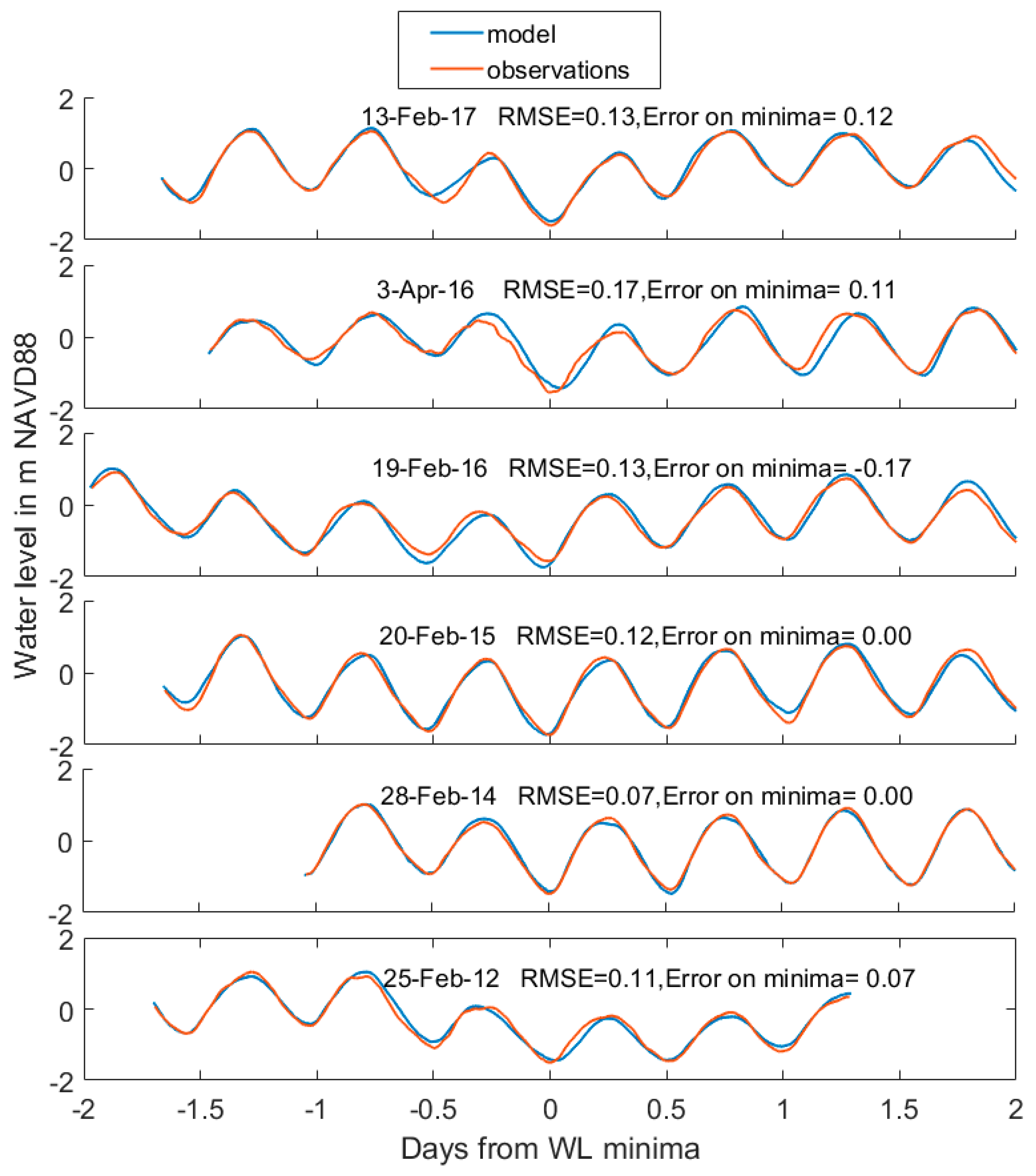
3.3. Hydrodynamic Modeling Methods and Water Level Validation

In this study, we use Stevens Estuarine and Coastal Ocean Model (SECOM), a three-dimensional (3D) hydrodynamic model based on the Princeton Ocean Model [29], subsequently ECOM [30]. SECOM is coupled with a surface wave model [23,31] and wind stress is computed using a wave-slope dependent sea surface drag coefficient [23,32], as done in recent studies, [33,34]. This is a curvilinear grid from Maryland to Cape Cod, encompassing the New York-New Jersey Harbor at its highest resolution of 25–100 m. The vertical resolution is 10 sigma layers. SECOM is also run with the New York Harbor Observing and Prediction System (NYHOPS) grid to operationally forecast and distribute warnings for floods and blowouts for the ensemble (probabilistic) Stevens Flood Advisory System (SFAS; [35]). The model application on this domain has been extensively validated for water level, current velocity, water temperature, and salinity [36,37,38,39].

To specifically evaluate the model’s capability to forecast and capture the mechanics of a blowout, the model is validated for six blowout events that occurred between 2012 and 2017 (Figure 3). The meteorological forcing for these simulations is obtained from forecasts created by NOAA from the Weather Research and Forecasting (WRF) model’s North American Mesoscale (NAM) domain application [40]. Streamflows, initial conditions, ocean boundary conditions, and model settings are all taken directly from operational NYHOPS forecast simulations [31,36,39]. This includes a high level of detail, with forecast data for 93 tributaries (National Weather Service Northeast River Forecast Center) and 426 other estimated freshwater and heat inputs within the domain. The model simulations compute the water levels beginning 24 hours before the peak of each blowout event. Raw model results are evaluated with a mean bias correction (the mean amplitude across events was 5 cm), which helps capture unresolved low-frequency sea level variations (e.g., seasonal variations [33]). This has little effect on our evaluation of the model’s capacity to capture the mechanics of negative surge.

The model validation for recent blowout events (Figure 3) shows very good accuracy, suggesting the model captures the primary physics of blowout events. The mean RMS error is 0.12 m across all six events, relative to mean water level minima of −1.56 m (NAVD88) at The Battery while the National Weather Service (NWS) defines an event as a blowout at The Battery if the water level is lower than −1.39 m. The average error on the minimum of the time series (at peak blowout) is 0.02 m. Occasionally there are tidal cycles with a phase difference between the observations and model output leading to higher errors (e.g., 3 April 2016; Figure 3). A possible cause of this minor and episodic mismatch is inaccuracies in the meteorological forcing (e.g., [23]).

3.4. Quantifying Blowout Sensitivities

The sensitivity of the water level to environmental factors is analyzed by experimenting with various meteorological and environmental conditions, including shore-fast surface ice on the Hudson, an ice jam in the north Hudson, and a wall in the East River. These environmental sensitivity model experiments are run with simplified scenarios and forcing. The model is run with typical moderate streamflows (for example—400 m³/s into the Hudson River at Troy, New York), though river streamflows have a relatively minor influence on sea level extrema at NYH [23]; moreover, any difference between the modeled and measured elevation caused by river flow is captured with the ~0.05 m bias correction described earlier (Section 3.3). Wind forcing for all sensitivity experiments is spatially uniform and imposed over the New York Bight, the continental shelf and all estuaries in the NYHOPS domain. Experiments using constant winds blowing over a larger area (a Northwest Atlantic domain developed by Orton et al. [33]) resulted in identical conclusions. Additional details of these experiments are described below.

3.4.1. Wind Stress-Tests

The objective of this experiment is to understand the sensitivity of surges to wind direction. 16 independent “wind stress-tests” are performed, each with wind blowing in a direction ranging from 0 to 337.5° in intervals of 22.5°. A wind direction is defined by the direction (or the angle from true north in degrees clockwise) from which the wind originates. Model simulations begin with 2 days of no wind; then, wind is ramped-up linearly to a peak magnitude of 18 m/s over a 12-h period, allowed to blow at that magnitude for 24 h, ramped-down to 0 m/s over 12 h, then left at 0 m/s for 24 h. The magnitude represents the largest observed at Newark Airport during a blowout during the past 60 years. The historical observed events are more variable, with elevated wind speeds for durations ranging from 12 to 30 h. Since the only variable forcing in this experiment is wind forcing (no tidal forcing), the water level reflects surge only. The results are discussed in Section 4.3.

3.4.2. Sensitivity to Altered Geometry and Environmental Factors (Emulating the Historical Changes)

After the wind direction stress-tests, the next set of experiments examines the sensitivity of the water levels in NYH to the evolving environment that was described in Section 2. We emulate four scenarios: An ice jam in the Hudson, reefs in the East River, altered surface friction due to shore-fast ice in the Hudson River north of New York City, and shallowing of the Ambrose shipping channel. These scenarios are run for five days in two sets of experiments—one with just west-northwest wind forcing as mentioned in 3.4.1 and another with the same wind forcing and a random tidal forcing (which was a snip of a real tidal time-series from the past). These experiments are called Surge and Tide experiments respectively.

(a)

An extreme case scenario of the reefs in the East River is emulated by building a wall near Hell Gate (shown as East River wall in Figure 1a). This is done by changing the depth to a negative value to extend out of the free-surface of the river. Hence, this wall stops the flow of water in and out of Hell Gate.

(b)

To emulate a choke point constraining the flow of water in the Hudson, an extreme case scenario is modeled in which an ice jam in the river would completely stop the flow of water to the south. The depth is changed to a negative value to replicate a dam in the grid cells across the river near West Point (shown in Figure 1a). West Point is chosen because it has been identified historically as a ‘choke point’ due to its tendency to form shore-fast ice cover which restricts ship traffic.

(c)

To mimic the impact of more commonly observed shore-fast ice cover, the surface ice friction is emulated by imposing a nominal horizontal drag coefficient at the free-surface, which is triple the bottom friction drag coefficient, to the grid cells in the Hudson to the north of 41.1° N, where shore-fast ice is commonly observed in wintertime. These surface drag coefficients were used by Georgas [14] to explain the tidal modulations due to ice cover in the Hudson River. Additionally, an extreme case scenario with a surface drag coefficient six times the bottom friction coefficient (twice the nominal value) is also tested.

(d)

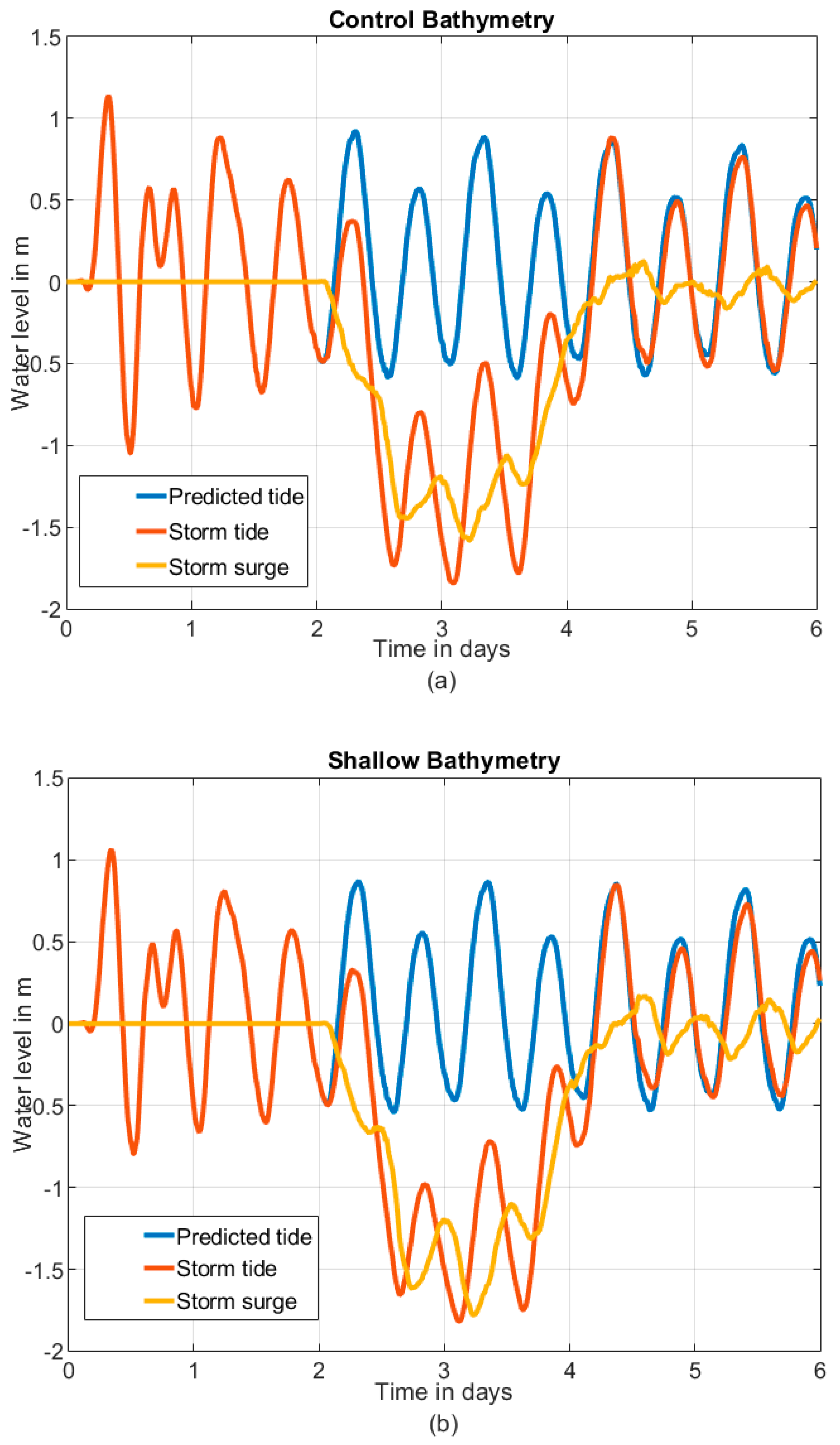
The historically-dredged shipping channels at the harbor entrance areas of Raritan Bay and Lower New York Bay south of latitude 40.56° N (Figure 1b) are shallowed in the model by setting the depth of the grid cells in the sections of the shipping channels deeper than six meters equal to six meters. This value is the approximate pre-dredging average bathymetric depth across the Ambrose Channel area, estimated from the Hassler Chart of NYH [18].

4. Results and Discussion

4.1. Historical Evolution of Blowouts

The annual minimum storm tides between 1860 and the present range from −2.05 m to −1.24 m (relative to local mean sea level) with a standard deviation of 0.15 m, whereas annual minimum storm surges range from −1.64 m to −0.68 m with a standard deviation of 0.18 m. By comparison, the measured range for positive storm tides and positive surges is 1.15 m to 3.38 m (standard deviation of 0.25 m), and 0.58 m to 2.67 m (standard deviation of 0.30 m), respectively (compare to [9,41]), where the large difference is caused by tropical cyclones. If only the non-hurricane season is considered (December through May), the Extra Tropical Cyclone (ETC) range for positive storm tide events is +1.19 m to +2.17 m (standard deviation of 0.19 m); hence, empirical data suggest a slight tendency for positive extratropical surges and storm tides to be larger than magnitude of negative surge and storm tides. The historical time series of annual minimum negative surge (Figure 4a) shows that extreme negative surges are weakening or are becoming ‘less frequent’ over the century. However, the historical time series of annual minimum storm tide (Figure 4b) does not show any apparent trend.

This historical change is quantitatively assessed in the extreme value analysis shown in Figure 5 which shows return period curves with 95% confidence intervals for negative surges (Figure 5a) and ELWs (Figure 5b). The magnitude of negative surges for most return periods (up to 50 years) are significantly larger in the first half of the dataset compared to the second half. For example, a negative surge of 1.35 m has a return period of 15 years in the first half (between 1860 and 1936) but has a return period of around 85 years in the second half (between 1937 and 2015). The magnitude of negative surge with return period of 10 years is around 13% higher in the first half (Figure 5a). However, we do not observe a significant difference in the blow-out storm tides (tide + surge) in the older half compared to the more-recent half of the data (Figure 5b). In Section 4.3, we present an idealized modeling approach and discuss the environmental factors in Section 4.4 that could have played a role in these historical trends.

4.2. Observed Meteorological Conditions for Blowout Events

The meteorological composite (Figure 6a) shows the sea level pressure and wind speed at 10 m, averaged over the top-25 negative surge events which are all cool-season extratropical cyclones. The meteorological composite shows that negative surge preferentially occurs when a low-pressure, extra-tropical cyclone occurs in northeastern Canada (Figure 6). Under these conditions, the isobars are oriented approximately from NW to SE in NYH, and a 10-m wind speed of about 14 m/s is observed over the mid-Atlantic Bight (Figure 6a). During these conditions, the composite average wind-direction at 10 m is 315° (Northwest) with an average wind speed around 12 m/s at the center of the nearest atmospheric reanalysis grid cell to NYH (the magenta asterisk in Figure 6a).

Station observations at Newark Airport show a similar, but slightly rotated, wind direction for the same blowout events. A radial histogram of the wind directions observed at Newark for all 25 events (Figure 6b) shows wind directions ranging from 240° to 330° with a modal direction around 290° over land (West-Northwest). This difference between isobar orientation in the composite and the modal direction in the histogram of observed wind directions could be explained by two factors, the winds in the composite being spatially averaged over a 0.7-degree resolution model grid cell (including both ocean and land areas) and the station-observed winds being rotated counter-clockwise by land-cover friction [42]. Results of the hydrodynamic modeling are used in the next section to comprehensively understand the sensitivity of surges to all the wind directions.

4.3. Model-Based Blowout and Storm Surge Sensitivity to Wind Direction

The wind stress-testing results show that west-northwest winds produce the most negative water levels in NYH (The Battery and Port Newark). Figure 7 shows two examples of the water level time series at all the locations for west-northwest wind (292.5° clockwise from north) and northwest wind (315°), which created the most negative water levels at NYH and in the Hudson River, respectively. From the water level time series at each location, the temporal minima (only the magnitude) and the maxima for all the wind directions are plotted in a polar diagram for the five locations (Figure 8).

The wind directions for blowout events from composite meteorological reanalysis and Newark Airport (Figure 6) suggest that Northwest or West-Northwest winds are optimal for negative surge at NYH, and similarly the optimal direction obtained by wind stress-testing with a constant wind forcing is West-Northwest. Any small rotational difference may be due to the historical wind data analyses being averaged at the apex of New York Bight with a variable wind forcing, whereas in the stress-test, the constant wind forcing acts over a larger scale. As isobars curve further out to sea (Figure 6a), winds correspondingly rotate counter-clockwise.

The polar diagrams (Figure 8) from the stress-test capture the directional sensitivity of positive and negative surges and show results that gradually rotate clockwise with distance up the Hudson River. Specifically, surge at the harbor entrance (Ambrose channel) is most sensitive to East/West directed winds, whereas up-river locations (e.g., West Point) are most sensitive to Northwesterly/Southeasterly winds. To examine how local harbor/estuary wind forcing relates to surge response, we define “fetch direction” as the direction of maximum fetch at a particular location in the harbor; at The Battery and Port Newark, fetch is aligned along a (22.5°; 202.5°) axis, at Haverstraw Bay and West Point, it is along (135°; 315°) and at Ambrose channel along (112.5°, 292.5°). Similarly, the wind directions causing strongest surges (positive and negative) are referred to as the “optimal wind directions”; at The Battery and Port Newark, the optimal wind directions are 112.5° and 292.5° for positive and negative surge, respectively. This is a rotation of 90° counter clockwise from the fetch direction. A similar counterclockwise rotation of 22.5° is observed at the Ambrose channel which is downstream of The Battery in Figure 8. However, at upstream locations like West Point and Haverstraw Bay, the optimal directions are parallel to the fetch directions. This rotation of optimal wind direction from the fetch direction is consistent with Coriolis force playing an important role remotely from the NY Bight, which was also shown in prior studies [23,43]. Moreover, this analysis also implies that the local wind setup and set-down are not major contributors to surge at these locations

We note that our result is affected by the time scale of our wind forcing. Ekman setup arising from the Coriolis force has a time scale of an inertial period of 18.4 h at this latitude (inertial period is approximated as 2 π/f where f is the Coriolis factor). The simulations studied here have a wind event time scale of 24 h (and an additional 12 h for wind spin-up and 12 h for spin-down), which is greater than this inertial period, and hence, the Coriolis force plays an important role. Additionally, we performed a preliminary sensitivity test to wind forcing time scale (12 h, 24 h, and 36 h, all with 12 h spin-up/down) which did not show any significant difference (results not shown). Lin et al. [43] showed that for NYC, a southeast wind (from 135°) is optimal for storm surge due to the geometry of New York Bight. We find a similar result for NYC (at The Battery) for the negative surge, but note that the optimal wind direction for both the positive and negative surge is spatially variable. Therefore, NYH blowouts for very short-duration wind events such as hurricanes would likely to be extreme for a northwest wind direction (315°), a slight rotation from our results (292.5°). This slight rotation in the results can be explained by the timescale of typical hurricane force winds, which lasts only a few hours (less than the inertial period). Hence, a short time scale surge is relatively less influenced by the Earth’s rotation.

Local wind stress forcing, and estuarine geometry appear to play an important modifying role, further up the Hudson River estuary. At Haverstraw Bay and West Point, the fetch directions are approximately along a (135°; 315°) axis, which is consistent with the optimal wind directions for surge. The increasing influence of local wind stress with distance up the estuary can explain the optimal wind directions rotating clockwise from Ambrose channel to West Point. Here, the local wind stress plays a larger role in the surge sensitivity compared to locations in NYH where remote wind effects from NY Bight dominate.

The magnitude of the peak negative surge increases by 50% from Ambrose Channel (1.2 m) northward up the Hudson (1.8 m at West Point). The increasing magnitude of surges up the Hudson is associated with the optimal wind direction for surge being more aligned with the fetch direction. This could be due to the substantial fetch along the estuary for winds blowing from the north, giving the local wind a larger role in producing a negative surge. In contrast, at locations in NYH the optimal wind directions are not aligned with the wind fetch direction; hence, local winds do not appear to play a role for the maximum observed surges. A likely additional factor here is the controlling effect of the relatively large volume and surface area of the nearby open ocean on any wind setup or set-down driven by local winds on the small surface area of NYH.

Interestingly, the magnitudes and directional sensitivity of positive and negative surges are near-mirror images of each other, suggesting that the physical controls on each are similar. Hence, asymmetries in estuary depth and wetted area (due to hypsometry) appear to play little role in setting negative and positive storm tide magnitudes, within the channel locations shown in Figure 8. This likely results from the Hudson being a relatively channelized and deep estuary, with only a small percentage of shallow areas (i.e., mean depth below 4 m) or intertidal zones. A similar result was shown by Drews [44] for the Gulf of Aqaba in Red sea basin.

4.4. Blowout Sensitivity to Environmental Factors

In this section, we discuss the sensitivity of blowouts to ice formation in the Hudson River and the presence of reefs in the East River. Sensitivity to change in bathymetry due to dredging is discussed in the next section. As mentioned in Section 3.3, these simulations are the extreme case scenarios of the historical observations like an ice jam in the Hudson and a wall in the East River and the water levels show some sensitivity to the changes made in the model grid. The surges for each of the scenario are compared with the control grid surges (

Table 1. Summary of the environmental sensitivity experiments with results for The Battery.

Experiment	Environmental Change	Anomaly of the Minima in Time Series (cm)
Surge experiments (Wind Only forcing)	Wall in the East River	+2.6
	Ice jam at West Point	+0.3
	Shallowing shipping channels	−7.3
Tide experiments (Wind + Tide forcing)	Ice jam at West Point	+1.1
	Shallowing shipping channels	+5.4
	Surface ice friction with twice nominal drag	+1.1

) and the following inferences are made.

(a)

East River wall: in the simulation with a west-northwest (WNW) wind, a wall in the East River increases the minimum water level in The Battery by a small amount (2.6 cm). This could be due to the wind stress driving the water in NYH from the west to east and up the East River. A presence of a wall could lead to accumulation of water in the East River and to a lesser extent near The Battery, hence increasing the water level locally.

(b)

Ice jam: in the case of an ice jam at West Point in the Hudson River, the wind driven water level minimum at The Battery also did not change substantially (Table 1). This could be due to the long distance from West Point to The Battery, which could spread out or attenuate any sea surface slope produced by the ice jam.

(c)

Ice friction sensitivity: the simulated ice-friction in the Hudson River produced a relatively insignificant effect (1 cm) on the water levels at The Battery (Table 1) even though the surface ice frictional coefficient was twice the normal value. Hence, we conclude that ice-friction did not play a major role in evolution of negative surges over the years in NYH. These results were qualitatively comparable to the findings of Georgas [14].

Due to the small changes found here, in these extreme scenarios which are greatly exaggerating the actual historical environment, we will not investigate these scenarios further.

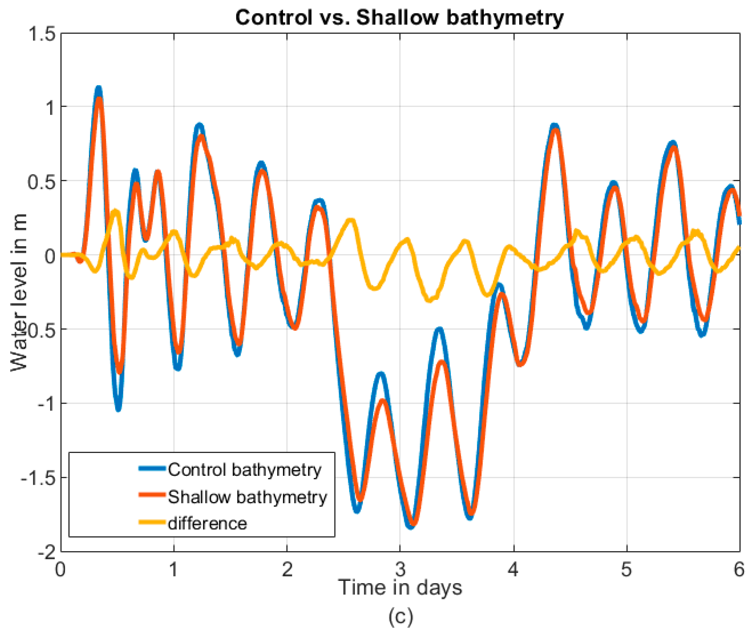
4.5. Bathymetric Sensitivity

Negative surges are more sensitive to changes in bathymetry compared to the total water levels. Figure 9 shows water levels and the surges during a blowout event. The most prominent change with the shallowed bathymetry before dredging (Figure 9b) compared to present bathymetry (Figure 9a) is that the minimum of the negative surge decreases by 20 cm (yellow lines). The weaker negative surge with present bathymetry (control) is consistent with the historical trend showing negative surges becoming less extreme over time (Figure 4 and Figure 5). By contrast, the minimum of the total water level is relatively unaffected by the shallowing of bathymetry (difference of 2 cm in the minimum as seen in Figure 9c). This occurs because the larger negative surges of the shallower historic bathymetry occur on a later (and thus, higher) phase of the predicted tide. This is also consistent with the historical records for annual minimum storm tide which did not show a significant change (Section 4.1).

Depth is a prime factor that influences propagation of tide and surge in shallow water, as well as their interaction [45,46]. The phase speed of an incoming long wave is dependent on depth in two ways—(1) directly from its shallow water wave properties which relate speed to the square root of depth times gravitational acceleration (${\mathit{c}}_{\mathit{o}}~\sqrt{\mathit{g}\mathit{h}}$), and (2) indirectly from bottom frictional effects [47], which modify wave speed [48,49]. As the depth of the water column is modified by dredging, it affects the speed of the incoming tide. This change in the speed of the tide wave induces a phase difference between the predicted tide and the actual tide, and that anomaly is perceived as an additional component of the “surge” (as it is typically defined; see [33]). This tide-surge interaction causes a tendency for large positive surges to occur on rising tides [33], as observed around the United Kingdom [45,50].

The same mechanistic argument can be used to explain how negative surge estimates are modulated with tide phase during a blowout. During a blow-out, winds drive the water level below the mean sea-level, which reduces the observed tidal phase speed below predicted values. During the falling tide, observed tide water levels are higher (fall later) than predicted, and low tide arrives late. Similarly, the subsequent rising tide is shifted later relative to predictions, such that a tide prediction over-estimates the actual tide water level. The residual difference between actual and predicted tide is positive during falling tide, and negative during rising tide:

$$\mathrm{Residual}=\mathrm{Actual}\mathrm{tide}-\mathrm{Predicted}\mathrm{tide}$$

Storm surge is calculated by:

$$\mathrm{Storm}\mathrm{surge}=\mathrm{Storm}\mathrm{tide}-\mathrm{Predicted}\mathrm{tide}$$

Combining the two equations demonstrates how this tide residual contributes to the estimate of the negative storm surge (as described in [46] for positive surge):

$$\mathrm{Storm}\mathrm{surge}=\mathrm{Storm}\mathrm{tide}-\mathrm{Actual}\mathrm{tide}+\mathrm{Residual}$$

From these considerations, we see that the largest apparent negative storm surge occurs when the residual is most negative, i.e., during a rising tide. This can be seen in historical time series data (e.g., Figure 2) where the surge minima often occur on a rising tide. The same is also observed in the model results for the bathymetric sensitivity analysis in Figure 9a,b).

Shallower bathymetry leads to a stronger tide-surge interaction response, for a given blowout event. The shallower the water, the greater the change in phase speed that is caused by the same change in depth. In turn, this produces a larger- phase difference between predicted and actual tide, residual between actual and predicted tides, and a larger apparent surge. For example, using the simple wave speed formula (${\mathit{c}}_{\mathit{o}}~\sqrt{\mathit{g}\mathit{h}}$) in water depth of 6 m, for a blowout decreasing 1 m of water level, the reduction in speed would be 8.7%, whereas for a depth of 15 m, the reduction in speed would be 3.4%. Hence, we can expect that the shallower bathymetry in the 1800s could give rise to more extreme negative surges than the present day (dredged) bathymetry, primarily due to this enhanced tide-surge interaction.

However, the idealized explanations discussed above do not consider tidal range variations and frictional tide-surge and tide-tide interactions. In realistic scenarios and the numerical model used here, the change in negative surge is due to a combination of tide phase shift and tidal range attenuation caused by tide-surge frictional interaction (compare blue lines in Figure 9a,b). However, for NYH, this attenuation has a relatively small effect on the resulting surge compared to the tide’s phase lag. For example, one consequence of depth changes is a shift in the relative phase (2Φ_M2–Φ_M4) between semidiurnal (M2) and quarter-diurnal (M4) constituents (e.g., [51,52]), or, more generally, the relative phase of all astronomical constituents and their non-linear overtides. Over time, the tide in NYH has become more symmetrical, and the average relative phase at The Battery changed from ~128° to ~137° between M2 and M4 between the 1860–1878 and 1998–2016 periods. When this change in relative phase and the slight decrease in M4 is considered, the downward shift in M4 curve is 2 mm (at high water, a symmetric increase of 2 mm occurs). Finally, when the M2 + M4 sum is considered, we find that total downward shift in predicted low water due to M2/M4 interaction is ~0.01 m (this occurs because M2 is slightly larger today). These slight changes are unlikely to greatly impact the magnitude of negative storm tide, nor alter the calculated surge.

Other factors, such as changing atmospheric parameters like wind speed, and atmospheric pressure, could also contribute to the evolution of negative surges, but we do not explore them in this paper. We also note that changes to damping within an estuary (caused by depth changes) often produce a large shift in tides and storm tide magnitudes (e.g., [13]). In NYH however, tides are not significantly damped, and changing bathymetry has only slightly altered the tidal range as can be seen in Figure 9c (also in [11]).

4.6. Amplification of Negative Surge Due to the Inverse Coastal Funneling Effect

A strong east-west gradient in the water levels can be seen in the negative surge map at Raritan Bay (Figure 10), and here we name this effect for blowouts as the Inverse Coastal Funneling Effect. The locations inside the bay have lower water levels than outside the bay, as shown in the map of the minimum negative surge for a west-northwest wind event. This is similar but in reverse to the funneling effect that has been observed for surges in bays or harbors with convergent coastline geometries, with amplification of the magnitude of surges [53]. It can be an important factor for funnel-shaped coastal areas where some ports and marinas are located at the apex of a bay, such as the New York Bight and the Raritan Bay area. An important consequence of this inverse funneling effect for NYH blowouts is that the surge minima at Port Newark are lower by 15 cm, relative to The Battery, which impacts the Port Newark. This is caused by the extremely low water levels at the apex of Raritan Bay causing a barotropic pressure gradient to drain the water from Newark Bay through Arthur Kill to the western end of Raritan Bay.

One simple reason why funnel shaped bays such as the Raritan Bay amplify positive or negative storm surges at their apex is suggested by mass balance requirements. In an idealized scenario with a spatially constant wind stress, wind stress affects a broader cross-section at the entrance to the bay, and a narrower cross-section near the apex. For a blowout, the resulting wind-driven mass transport integrated across the wider cross-section is larger than near the apex, causing a divergence and a sharp drop in water level at the apex. In Raritan Bay, we computed the sea level slope based on water depth, bed stress and wind stress alone (from a steady-state vertically-integrated momentum budget; see p. 156 in [5]), and we found that the modeled result was nearly twice this value, consistent with there being an amplification effect.

Oftentimes, negative and positive surges come in close proximity, caused by a single hurricane or extratropical cyclone [54]. Due to the amplification of both positive and negative surges, this could produce particularly rapid swings in sea level, strong water velocities, and hazardous conditions for ships that are sheltering from the storm in an embayment.

5. Summary and Conclusions

In this paper, an important but rarely explored aspect of coastal sea level extremes called blowouts was analyzed. An improved understanding and modeling of blowouts is useful to improve our predictive capacity for both positive and negative sea level extremes, improving coastal safety. Moreover, ELW events can carry high costs for the maritime industry with unforeseen delays or dangerous groundings, if not accurately predicted. They can also be a concern for the safety of uninformed boaters, recreational fishermen, and nuclear power plants and other facilities that require water for cooling systems. Experiments and historical data were utilized to explore the mechanics of negative surges and ELWs in NYH, and their evolution over the century.

We analyzed the water level records from 1860 to 2015 to study trends in the negative surges and ELWs during blowout events in NYH. The water level records show that negative surges have been less extreme in recent decades, yet ELWs have shown no apparent long-term change. We quantified the historical change in blowout extremes using statistical extreme value analysis. The extreme value analysis showed that the negative surges were higher in magnitude in the past compared to the present.

We assessed the sensitivity of blowouts to (a) wind direction, (b) ice formation in the Hudson River, (c) reefs in the East River, and (d) deepening of bathymetry in the shipping channels due to dredging using experiments with the hydrodynamic model. The most important factor was the change in bathymetry due to dredging which changes the negative surges in NYH while the other factors tested play an insignificant role. This is due to the difference between the predicted and the observed tide caused by the reduction of the phase speed of the observed tide because of decrease in the depth. While not taking all the meteorological variables exhaustively into account, we partially attributed the historical trends in negative surges to the changing depth in NYH.

We performed a set of experiments for sensitivity analysis of the surges to wind direction. This was then compared with the meteorological data from observed blowout events. The wind sensitivity experiments showed that a west-northwest wind is most efficient in producing the lowest water levels in a blowout event in NYH. These experiments showed a spatial variability in sensitivity of surges to wind direction. They also suggested a dominance of remote (offshore) wind effects through Coriolis force in influencing the water levels in NYH, but the dominance decreases upstream in the Hudson where the local wind stress dominates the water levels.

Positive and negative surges have very similar mechanics in NYH, but in reverse direction, as reflected in the near-symmetry of their wind sensitivities. The asymmetries due to local wind effects arising from geometry and depth are concealed by the much stronger influence of large scale forcing. This observation can also be seen in the phenomena of tide-surge interaction and the funneling effect where surge is accentuated at the apex of a funnel-shaped bay. Hence, it is the large-scale forcing that is important in this system; any asymmetry between positive and negative surge is being caused by weather patterns, rather than local geometric effects.

References

1. Schureman, P. Tides and Currents in Hudson River; Citeseer: Washington, DC, USA, 1934. [Google Scholar]
2. Pittman, C. Why Irma drained the water from Tampa Bay. Available online: http://www.tampabay.com/opinion/columns/pittman-why-irma-drained-the-water-from-tampa-bay/2338244 (accessed on 13 May 2019).
3. McWhirter, C.; Campo-Flores, A. U.S. Ports See Costly Delays as Cargo Ships, Volumes Grow. Available online: https://www.wsj.com/articles/u-s-ports-see-costly-delays-as-cargo-ships-volumes-grow-1430340113 (accessed on 13 May 2019).
4. Sobey, R.J. Extreme low and high water levels. Coast. Eng. 2005, 52, 63–77. [Google Scholar] [CrossRef]
5. Pugh, D.; Woodworth, P. Sea-Level Science: Understanding Tides, Surges, Tsunamis and Mean Sea-Level Changes; Cambridge University Press: Cambridge, UK, 2014. [Google Scholar]
6. Resio, D.T.; Westerink, J.J. Modeling the physics of storm surges. Phys. Today 2008, 9, 33–38. [Google Scholar] [CrossRef]
7. Raicich, F. Recent evolution of sea-level extremes at Trieste (Northern Adriatic). Cont. Shelf Res. 2003, 23, 225–235. [Google Scholar] [CrossRef]
8. Pugh, D.T.; Vassie, J.M. Extreme Sea Levels from Tide and Surge Probability. In Coastal Engineering 1978; Institute of Ocwanographic Science: Merseyside, UK, 1978. [Google Scholar]
9. Talke, S.; Orton, P.; Jay, D. Increasing storm tides at New York City, 1844–2013. Geophys. Res. Lett. 2014, 41, 3149–3155. [Google Scholar] [CrossRef]
10. Chant, R.J.; Sommerfield, C.K.; Talke, S.A. Impact of Channel Deepening on Tidal and Gravitational Circulation in a Highly Engineered Estuarine Basin. Estuaries Coasts 2018, 41, 1587–1600. [Google Scholar] [CrossRef]
11. Ralston, D.K.; Talke, S.; Geyer, W.R.; Al-Zubaidi, H.A.; Sommerfield, C.K. Bigger tides, less flooding: Effects of dredging on barotropic dynamics in a highly modified estuary. J. Geophys. Res. Ocean. 2019, 124, 196–211. [Google Scholar] [CrossRef]
12. Orton, P.M.; Talke, S.A.; Jay, D.A.; Yin, L.; Blumberg, A.F.; Georgas, N.; Zhao, H.; Roberts, H.J.; MacManus, K. Channel Shallowing as Mitigation of Coastal Flooding. J. Mar. Sci. Eng. 2015, 3, 654–673. [Google Scholar] [CrossRef] [Green Version]
13. Familikhalili, R.; Talke, S.A. The effect of channel deepening on tides and storm surge: A case study of Wilmington, NC. Geophys. Res. Lett. 2016, 43, 9138–9147. [Google Scholar] [CrossRef] [Green Version]
14. Georgas, N. Large Seasonal Modulation of Tides due to Ice Cover Friction in a Midlatitude Estuary. J. Phys. Oceanogr. 2012, 42, 352–369. [Google Scholar] [CrossRef]
15. Marcos, M.; Woodworth, P.L. Spatiotemporal changes in extreme sea levels along the coasts of the North Atlantic and the Gulf of Mexico. J. Geophys. Res. Ocean. 2017, 122, 7031–7048. [Google Scholar] [CrossRef]
16. Field, A.M. Port Productivity: The Cooperation Revolution at the Port of New York and New Jersey. J. Commer. 2015. Available online: https://www.joc.com/sites/default/files/u59196/Whitepapers/NYNJ_PortProductivity/WP-NYNJ-v4-agbJAY.pdf (accessed on 23 March 2019).
17. Ascher, K. Going Up! A Bridge Makes Way for Bigger Ships. The New York Times, 2014. Available online: https://www.nytimes.com/2014/03/23/nyregion/going-up-a-bridge-makes-way-for-bigger-ships.html(accessed on 23 March 2019).
18. Hassler, F.R. Map of New-York Bay and Harbor and the Environs; United States Coast Survey: Washington, DC, USA, 1844. [Google Scholar]
19. Keegan, G.C. The Dredging Crisis In New York Harbor: Present and Future Problems, Present and Future Solutions. Fordham Environ. Law J. 1997, 8, 351–388. [Google Scholar]
20. United States Army Corps of Engineers. Report of the Chief of Engineers, U.S. Army; U.S. Government Printing Office: Washington, DC, USA, 1920.
21. American Society of Civil Engineers. Transactions of the American Society of Civil Engineers; American Society of Civil Engineers: Reston, VA, USA, 1921. [Google Scholar]
22. USACE Fact Sheet—New York and New Jersey Harbor Deepening. Available online: http://www.nan.usace.army.mil/Media/Fact-Sheets/Fact-Sheet-Article-View/Article/487407/fact-sheet-new-york-new-jersey-harbor-50-ft-deepening/ (accessed on 13 May 2019).
23. Orton, P.; Georgas, N.; Blumberg, A.; Pullen, J. Detailed modeling of recent severe storm tides in estuaries of the New York City region. J. Geophys. Res. 2012, 117, C09030. [Google Scholar] [CrossRef]
24. Georgas, N.; Miller, J.; Wang, Y.; Jian, Y.; D’Agostino, D. Tidal Hudson River Ice Cover Climatology; Hudson River Sustainable Shorelines Project: Staatsburg, NY, USA, 2015. [Google Scholar]
25. Pawlowicz, R.; Beardsley, B.; Lentz, S. Classical tidal harmonic analysis including error estimates in MATLAB using T_TIDE. Comput. Geosci. 2002, 28, 929–937. [Google Scholar] [CrossRef]
26. Leffler, K.E.; Jay, D.A. Enhancing tidal harmonic analysis: Robust (hybrid L1/L2) solutions. Cont. Shelf Res. 2009, 29, 78–88. [Google Scholar] [CrossRef]
27. Dee, D.P.; Uppala, S.M.; Simmons, A.; Berrisford, P.; Poli, P.; Kobayashi, S.; Andrae, U.; Balmaseda, M.; Balsamo, G.; Bauer, D.P. The ERA-Interim reanalysis: Configuration and performance of the data assimilation system. Q. J. R. Meteorol. Soc. 2011, 137, 553–597. [Google Scholar] [CrossRef]
28. NOAA Center for Operational Oceanographic Products and Services. Available online: https://tidesandcurrents.noaa.gov/ (accessed on 11 May 2019).
29. Blumberg, A.F.; Mellor, G.L. A description of a three-dimensional coastal ocean circulation model. In Three-Dimensional Coastal Ocean Models; Heaps, N.S., Ed.; American Geophysical Union: Washington, DC, USA, 1987; Volume 4, pp. 1–16. [Google Scholar]
30. Blumberg, A.F.; Khan, L.A.; St John, J. Three-dimensional hydrodynamic model of New York Harbor region. J. Hydraul. Eng. 1999, 125, 799–816. [Google Scholar] [CrossRef]
31. Georgas, N.; Blumberg, A.; Herrington, T. An operational coastal wave forecasting model for New Jersey and Long Island waters. Shore Beach 2007, 75, 30–35. [Google Scholar]
32. Taylor, P.K.; Yelland, M.J. The dependence of sea surface roughness on the height and steepness of the waves. J. Phys. Oceanogr. 2001, 31, 572–590. [Google Scholar] [CrossRef]
33. Orton, P.; Hall, T.M.; Talke, S.; Blumberg, A.F.; Georgas, N.; Vinogradov, S. A Validated Tropical-Extratropical Flood Hazard Assessment for New York Harbor. J. Geophys. Res. 2016, 121, 8904–8929. [Google Scholar] [CrossRef]
34. Georgas, N.; Yin, L.; Jiang, Y.; Wang, Y.; Howell, P.; Saba, V.; Schulte, J.; Orton, P.; Wen, B. An Open-Access, Multi-Decadal, Three-Dimensional, Hydrodynamic Hindcast Dataset for the Long Island Sound and New York/New Jersey Harbor Estuaries. J. Mar. Sci. Eng. 2016, 4, 48. [Google Scholar] [CrossRef]
35. Jordi, A.; Georgas, N.; Blumberg, A.; Yin, L.; Chen, Z.; Wang, Y.; Schulte, J.; Ramaswamy, V.; Runnels, D.; Saleh, F. A next-generation coastal ocean operational system: Probabilistic flood forecasting at street scale. Bull. Am. Meteorol. Soc. 2018. [Google Scholar] [CrossRef]
36. Georgas, N.; Blumberg, A.F. Establishing confidence in marine forecast systems: The design and skill assessment of the New York Harbor Observation and Prediction System, version 3 (NYHOPS v3). In Proceedings of the 11th International Conference on Estuarine and Coastal Modeling, Seattle, WA, USA, 4–6 November 2009; pp. 660–685. [Google Scholar]
37. Di Liberto, T.; Colle, B.A.; Georgas, N.; Blumberg, A.F.; Taylor, A.A. Verification of a multimodel storm surge ensemble around New York City and Long Island for the cool season. Weather Forecast. 2011, 26, 922–939. [Google Scholar] [CrossRef]
38. Kuang, L.; Blumberg, A.F.; Georgas, N. Assessing the fidelity of surface currents from a coastal ocean model and HF radar using drifting buoys in the Middle Atlantic Bight. Ocean Dyn. 2012, 62, 1229–1243. [Google Scholar] [CrossRef]
39. Georgas, N. Establishing Confidence in Marine Forecast Systems: The Design of a High Fidelity Marine Forecast Model for the NY/NJ Harbor Estuary and Its Adjoining Coastal Waters. Ph.D. Thesis, Department of Civil, Environmental and Ocean Engineering, Stevens Institute of Technology, Hoboken, NJ, USA, 2010. [Google Scholar]
40. NOAA National Centers for Environmental Information. Available online: https://www.ncdc.noaa.gov/data-access/model-data/model-datasets/north-american-mesoscale-forecast-system-nam (accessed on 11 May 2019).
41. Colle, B.A.; Rojowsky, K.; Buonaito, F. New York City Storm Surges: Climatology and an Analysis of the Wind and Cyclone Evolution. J. Appl. Meteorol. Climatol. 2010, 49, 85–100. [Google Scholar] [CrossRef]
42. Kusuda, M.; Alpert, P. Anti-Clockwise Rotation of the Wind Hodograph. Part I: Theoretical Study. J. Atmos. Sci. 1983, 40, 487–499. [Google Scholar] [CrossRef] [Green Version]
43. Lin, N.; Emanuel, K.; Smith, J.; Vanmarcke, E. Risk assessment of hurricane storm surge for New York City. J. Geophys. Res 2010, 115. [Google Scholar] [CrossRef]
44. Drews, C. Directional Storm Surge in Enclosed Seas: The Red Sea, the Adriatic, and Venice. J. Mar. Sci. Eng. 2015, 3, 356. [Google Scholar] [CrossRef]
45. Prandle, D.; Wolf, J. The interaction of surge and tide in the North Sea and River Thames. Geophys. J. Int. 1978, 55, 203–216. [Google Scholar] [CrossRef] [Green Version]
46. Horsburgh, K.; Wilson, C. Tide-surge interaction and its role in the distribution of surge residuals in the North Sea. J. Geophys. Res. Oceans 2007, 112, C8. [Google Scholar] [CrossRef]
47. Parker, B.B. Frictional Effects on the Tidal Dynamics of a Shallow Estuary. Ph.D. Thesis, Johns Hopkins University, Baltimore, MD, USA, 1984. [Google Scholar]
48. Wolf, J. Surge-tide interaction in the North Sea and River Thames. Floods Due High Wind. Tides 1981, 75–94. [Google Scholar]
49. Jay, D.A. Green’s law revisited: Tidal long-wave propagation in channels with strong topography. J. Geophys. Res. Ocean. 1991, 96, 20585–20598. [Google Scholar] [CrossRef]
50. Rossiter, J.R. Interaction between tide and surge in the Thames. Geophys. J. Int. 1961, 6, 29–53. [Google Scholar] [CrossRef]
51. Friedrichs, C.T.; Aubrey, D.G. Non-linear tidal distortion in shallow well-mixed estuaries: a synthesis. Estuar. Coast. Shelf Sci. 1988, 27, 521–545. [Google Scholar] [CrossRef]
52. Chernetsky, A.S.; Schuttelaars, H.M.; Talke, S.A. The effect of tidal asymmetry and temporal settling lag on sediment trapping in tidal estuaries. Ocean Dyn. 2010, 60, 1219–1241. [Google Scholar] [CrossRef] [Green Version]
53. As-Salek, J.A. Coastal trapping and funneling effects on storm surges in the Meghna estuary in relation to cyclones hitting Noakhali-Cox’s Bazar coast of Bangladesh. J. Phys. Oceanogr. 1998, 28, 227–249. [Google Scholar] [CrossRef]
54. Pousa, J.L.; D’Onofrio, E.E.; Fiore, M.M.E.; Kruse, E.E. Environmental impacts and simultaneity of positive and negative storm surges on the coast of the Province of Buenos Aires, Argentina. Environ. Earth Sci. 2013, 68, 2325–2335. [Google Scholar] [CrossRef]
Figure 1. (a) Locations and tide gauges referred to in this paper; (b) bathymetry of the central New York Harbor (NYH) region used in modeling (as gridded for the numerical model used in this paper).
Jmse 07 00160 g001
Figure 2. Time Series of water level in m (a) at The Battery for an Extra Tropical Cyclone (ETC) on 1/10/1978 with the historically largest extreme low water (ELW); and (b) at Governor’s Island for an ETC on 2/25/1862 with the historically largest negative surge. “Prediction” is the astronomical tide prediction.
Jmse 07 00160 g002
Figure 3. Hindcast simulations for six recent blowout events, showing water level at The Battery.
Jmse 07 00160 g003
Figure 4. (a) Time series of annual minimum negative surges; (b) annual minimum storm tide (relative to local mean sea level) from 1860–2015 compiled from various tide gauge stations in NYH. The annual mean sea level has been subtracted to remove the effects of sea level-rise.
Jmse 07 00160 g004
Figure 5. (a) Return period curve for exceedance of negative surges (absolute value), with data divided into older and more recent periods; (b) return period curve for exceedance of negative water level, similarly. All cases show 95% confidence intervals with dashed lines.
Jmse 07 00160 g005
Figure 6. (a) Meteorological composite of conditions for top 25 negative surge events (1979–2014), including wind speed shading in m/s (10 m elevation) and sea level pressure isobars (with 5 hPa intervals). (b) Radial histogram for the three-hour averaged observed wind directions for the same events from Newark Airport, the color shading shows the wind speed in m/s. Meteorological data from 6 h prior to minimum surge are used for both panels, which accounts for the typical lag seen in our modeling between regional winds and the resulting negative surge at The Battery.
Jmse 07 00160 g006
Figure 7. Modeled surge time series at several locations for (a) the 18 m/s west-northwest wind stress-test; and (b) for the 18 m/s northwest wind stress-test.
Jmse 07 00160 g007
Figure 8. Maximum surges (orange) and minimum negative surges (blue) from separate stress-test simulations with 16 directions of wind. Radial axes are water level in m. Temporal minima and maxima from datasets like those in Figure 7 are plotted for all 16 wind directions at the five locations.
Jmse 07 00160 g008
Figure 9. Time series of water level (storm tide) and surge during a blowout event using a random tide. Panels show: (a) simulation results for a tide/west wind simulation with control bathymetry; (b) results with shallow bathymetry; and (c) time series of total water levels for control bathymetry and shallow bathymetry, and the difference between the two.
Jmse 07 00160 g009aJmse 07 00160 g009b
Figure 10. Map showing color-shaded minimum storm surge (m) in time series for a west-northwest wind event, with no tidal forcing. Wind forcing is the same as that used for Figure 7.
Jmse 07 00160 g010