Mathematical Modeling Framework of Physical Effects Induced by Sediments Handling Operations in Marine and Coastal Areas

Abstract

In recent years increasing attention has been paid to environmental effects that may result from marine dredging and disposal operations. In general, the fine-grained fraction of handled sediments can be dispersed far from the intervention site as a turbidity plume, depending on the specific site and operational parameters. Starting from a literature review, this paper suggests standards for estimating and characterizing the sediment source term, for setting up far-field modeling studies and analyzing numerical results, with the aim of optimizing, also from an economic point of view, the different project, execution and monitoring phases. The paper proposes an integrated modeling approach for simulating sediment dispersion due to sediment handling operations in different marine-coastal areas (off-shore, near-shore and semi-enclosed basins). Attention is paid to the characterization of sediment source terms due to different operational phases (removal, transport and disposal). The paper also deals with the definition of accuracy level of modeling activities, with regard to the main physical processes characterizing the different marine–coastal areas and to the type of environmental critical issues near the intervention site (if any). The main relationships between modeling and monitoring are given for the different design and management phases to support the selection of appropriate technical alternatives and monitoring actions and to ensure the environmental compliance of the proposed interventions.

1. Introduction

Interventions in marine and coastal areas often involve sediment dredging and disposal operations. The volume of sediments handling can vary in relation to the operations purposes, e.g., to maintain or improve the navigation depth of ports and harbors (e.g., [1]), for creating or improving facilities (e.g., [2]), for beach nourishment (e.g., [3]) and open-water disposal (e.g., [4]), to carefully remove and relocate contaminated materials (e.g., [5]) or morphological reconstruction in transitional areas. Moreover, the operational techniques (e.g., type and capacity of dredges) are key aspects to be accounted for when dealing with the assessment of physical effects due to sediment handling works (e.g., [6,7]).

Pre-approval from controlling authorities is typically required to verify environmental and economic compatibility of equipment, work plans and operational criteria prior to the initiation of the activities. The approval requirements include the evaluation of short-term effects occurring during the project phases (often referred to as process effects) and long-term effects caused by the final project layout (often referred to as project effects, e.g., [8]).

For the European Union, detailed environmental impact assessment (Directive 2014/52/UE, [9]) are aimed at selecting technical alternatives and designing appropriate mitigation measures and monitoring actions for ensuring environmental compliance, especially when either large quantities or polluted sediments have to be handled. Far from the intervention areas the dispersal and settling of plumes of spilled sediment can induce a broad range of effects, i.e., light reduction and sedimentation at sensitive receptors, changes in abundance, diversity and biomass of seabed habitats and benthic communities, contaminants and nutrients release. An efficient management of sediment handling works requires knowledge both of the operational factors (i.e., extension of dredging/disposal areas, kinematic and geometric parameters of dredging/disposal techniques, duration and timing of operations) to assess the sediment release mechanisms, and of the site conditions (i.e., sediment type, water depth, currents and waves climates, thermohaline stratification, seasonal window) to assess the spatial dispersion and the settling time of the sediment plume during and after the end of operations.

In this framework, mathematical models are recognized as a valuable tool to forecast the plume dynamics and the areas interested by significant variations of suspended sediment concentration (SSC) and sediment deposition rates (DEP, e.g., [10,11,12]). Recent research (e.g., [13]) and international guidelines (e.g., [14]) often include the use of mathematical models to perform environmental studies needed to support decision makers (before, during and after execution) to optimize the interventions and monitoring actions with regard to environmental and project objectives [15], while maintaining desired production rates [16]. A major effort has been put to support contractors and controlling authorities to combine modeling and monitoring activities in a feedback framework [15,17,18]. This is aimed (i) at assessing and approving dredging equipment and work plans (prior to the operations start), and (ii) at introducing assessment procedures based on the application of environmental criteria, for ensuring that SSC remains below specified limits (during the operations) and for timely changing work plans and monitoring frequencies to prevent any potential short- and long-term environmental effects (during and after the operations).

Common modeling approaches involves hydrodynamic and transport models suitable to quantify and to compare the transport processes of the different spilled sediment, moving from the near- to the far-field (e.g., [11,12,19,20]). Nevertheless, technical and scientific literature highlights the lack of an organic and comprehensive methodology driving the selection of appropriate modeling tools and of accuracy levels needed for a reliable assessment of the induced physical effects in different environmental contexts and when environmental critical issues are involved (e.g., ecological sensitive receptor, water quality, sensitive habitat and species, fish farming facilities, regulatory constraints, etc.). In the context of national experiences, the Italian National Institute for Environmental Protection and Research (ISPRA) issued the Italian Guidelines dealing with the modeling approach that can be implemented in relation both to environmental and project objectives, promoting uniform procedures for different techniques, operational phases, and environmental contexts [15].

For ensuring the compliance with environmental requirements, the selection of a modeling approach must balance the accuracy of results related to strict environmental critical issues and operating criteria defined prior the initiations of the operations. Moreover, input data for the selected modeling scenarios should be appropriate for a reliable representation of the main physical processes variability driving the dynamic of the plume during the different operational phases, depending on the main characteristics of the selected techniques. It has to be stressed that past studies (e.g., [14,21,22]) found that results rarely focus on long-term effects of sediments dispersion, within either seasonal or annual time windows. Rather, they are focused on short-term scenarios usually related to either one or few tidal cycles or extreme events (e.g., [23,24,25]).

Increases of SSC and DEP away from the re-suspension source are mainly used to evaluate the extension of the area affected by plume dispersion, where the maximum SSC is usually expressed in relation to given thresholds. It has to be stressed that there is also a lack of tools that synthesize and make the modeling results useful for supporting decision system and environmental management [22] and to give operational and environmental indications to optimize all the planning and management phases of the sediment handling project.

GBRMPA [14] and Feola et al. [26] recommend that model results should be synthesized by means of maps showing statistical measures (i.e., maximum and mean) of the predicted SSC and DEP at different water depths, as well as by the synthetic parameters of the time series at different key sites, intended to be representative of the environmental context and of the duration of the project. It is suggested to analyze environmental effects in terms of the duration of the time windows during which given SSC thresholds are exceeded during the operations [16].

Starting from a literature review, this paper suggests standards for both setting up modeling and field studies and for analyzing and assessing modeling results with regards to: (i) areas of intervention (coastal areas, semi-enclosed basins and offshore areas), (ii) operational phases (excavation, loading/transport and disposal), (iii) operational techniques (hydraulic and mechanical dredges), and (iv) environmentally sensitive critical issues (if any). For sake of clarity, the key points of this paper are:

• an organic and comprehensive framework about the physical effects induced by sediments handling operations is proposed;
• a broad-spectrum modeling approach intended to support contractors and controlling authorities in planning and managing sediment handling operations is detailed;
• an integrated, flexible and replicable methodological approach for synthesizing numerical results is illustrated;
• the main features of the required modeling–monitoring feedback system are highlighted.

This paper is structured as follows. Section 2 aims at describing the proposed methodological approach. Section 3 and Section 4 detail the rationale for the selection of scenarios and the source term definition respectively. Section 5 and Section 6 illustrate the proposed integrated modeling approach for simulating sediment dispersion, intended as a general framework to assess the physical effects of sediments handling operation, thus by identifying areas interested by significant changes in terms of physical parameters (e.g., SSC and DEP) due to plume dynamics, and from which environmental risk can be derived. Also, the relationship between modeling and monitoring activities for proper implementation and verification both of modeling studies and of decision processes in different project phases are outlined (Section 8.1), and the importance of the management and sharing of monitoring data is highlighted (Section 8.2). Concluding remarks close the paper.

2. The Proposed Modeling Approach

This paper provides an organic and comprehensive framework about the physical effects induced by sediments handling operations and proposes a broad-spectrum modeling approach intended to support contractors and controlling authorities in planning and managing such a kind of interventions. Hereinafter, the plume dynamics are intended to be related either to removal or disposal induced re-suspension/release of the fine fraction of the handled sediments, as well as to advection, deposition and sometimes re-suspension from the bottom due to environmental forcing. The whole sediment handling work cycle is described by different operational phases: removal (or excavation), loading, transport and disposal of handled sediments. Moreover, different environmental contexts (coastal areas, semi-enclosed basins and offshore areas) are considered as intervention areas.

Even if the water depth, respectively in shallow or deep offshore areas, may induce operational differences in excavation and disposal, these distinctions are not addressed in this paper. Indeed, as also suggested by Marine Strategy Framework Directive 2008/56/EC [27], the area of interest should be defined taking into account the strict interaction between off-shore and near-shore hydrodynamics. Then, the area of interest could reach the national limits and beyond, of course with an appropriate and feasible spatial scale. Hence, all the main physical phenomena influencing the dynamics of the induced sediment plumes can be properly modeled.

Mathematical models, calibrated and validated through the use of literature and field data, are recognized as useful supporting tools to plan, design and manage sediment handling operations. In particular, they can support the comparative choice of the technical and operational alternatives based on the forecast of possible environmental issues. The reliable estimation of the physical processes characterizing the sediment plume dynamic during the whole handling cycle requires the selection of mathematical models able to reproduce the primary physical features of the intervention area, of the project goals, and of the environmental aspects. The proper model selection and implementation require the definition of the main hydrodynamic field and source term features driving the spatial and temporal variability of dispersal of the spilled sediment and contamination processes (if any). Similarly, the selected approach for the numerical solution of the governing equations for hydrodynamic and transport phenomena influences the burden in terms of resources, computational times and of required input data.

The proposed integrated modeling approach relies on standard numerical suites worldwide used to model the passive phase of plume dispersion, but the source term definition aimed at accounting for the near-field processes, at least from a macro-scale point of view. Three numerical modules, hereinafter referred to as the hydrodynamic module (H-M in Figure 1), source term module (ST-M in Figure 1) and transport module (T-M in Figure 1) are implemented in series. Basically, the transport module is used to estimate SSC and DEP resulting from dispersion of the sediment release (estimated by the source term module) due to the flow field variability (estimated by the hydrodynamic module). Then, an environmental assessment module (EA-M in Figure 1) provides standard methods and statistical parameters for the assessment of the physical environmental effects. A modeling–monitoring feedback system is then recommended and considered as an integral part of the proposed integrated modeling approach. With the aim to define a proper modeling setup, validation of modeling results and verifying when sediment spill exceeds specified limits. These limits, hereinafter referred to as reference levels, are intended to be defined with respect to the natural background conditions and to the environmental critical issues types (if any).

Lisi et al. [15] suggest that the modeling studies should be performed in different steps, with increasing level of detail, and they give practical indications to optimize the work plan, with regard to environmental and operational site-specific objectives. The accuracy of quantitative estimates depends on the used modeling approach (modeling tools and scenarios), and it is a function of the expected results. Indeed, depending on the project phase (i.e., prior, during or after), different detail levels can be required. Furthermore, this also makes the proposed methodology feasible from an economic point of view (Figure 2). It is argued that expert judgment should be the first effort performed. A preliminary information phase aims at selecting reference conditions to assess when modeling approaches are needed and to define their accuracy level with respect to environmental expected effects. Within this phase, based on operative and environmental data collection, scientists with different expertise should be engaged within the framework of a holistic approach. When the preliminary information phase highlights that significant environmental effects are likely to occur, the implementation of modeling studies is recommended for their estimation. In these cases, the next step is the implementation of a preliminary modeling phase, in which simplified models are used to describe the key features of the plume dynamic and allow a fast estimation of its expected maximum extension area. The reader is referred to Section 5 for details on preliminary information phase and preliminary modeling phase. A detailed modeling phase (see Section 6 for details) is then suggested when the preliminary modeling phase confirms that the dispersion of spilled sediment can impact on water quality and on the site-specific environmental targets. It is intended to allow accurate evaluations even for complex conditions.

The detailed modeling phase is always recommended when three-dimensional features (for source terms and/or hydrodynamic patterns) play a key role and when environmental critical issues are revealed and/or predicted by preliminary modeling phase. It has to be stressed that the preliminary modeling phase plays an important role even when detailed modeling is implemented, in order to evaluate the possible need and the nature of detailed analysis and to support the preliminary assessment of the worst-case scenarios (e.g., extreme events or mitigation failure). This is aimed at optimizing the work plan and the approval procedures, with regard to environmental and operational site-specific objectives. Figure 2 depicts the flow chart of the proposed general approach.

Some initial modeling assumptions (e.g., within the preliminary information phase and preliminary modeling phase) may vary during the project development (e.g., from the planning phase up to the execution). Indeed, it may be observed that key information could not well defined at the preliminary design phase of a sediment handling project, while it is (or should be at least) known at a later stage. According to the adaptive management approach [17], a stepwise procedure can address uncertainties as the project progresses, incorporating flexibility and robustness into project design, and using latest information to instruct decision-makers as the project develops.

3. Scenarios

The selection of the scenarios to be modeled plays a crucial role in the choice of the mathematical models and also on the reliability of the modeling results obtained for the relevant physical phenomena.

Herein, four different modeling scenarios are proposed and detailed for driving the proper implementation of the proposed integrated modeling approach (

Table 1. Main features of the modeling scenarios proposed within the different accuracy levels of the proposed integrated approach.

Approach	Aim	Limitations	Needed Data
Climatological	To reproduce specific conditions not directly related to measured data, e.g., to specific Average Return Period.	The marginal occurrence probability (i.e., simultaneity of driving forces) is seldom reproduced.	Results of statistical analyses (e.g., of either atmospheric or hydrodynamic forcing).
Short-term realistic	To reproduce specific conditions observed in the past in order to take into account the simultaneity of different driving forces. The results can be used for numerical models validation.	The needed data are seldom available, in particular during the preliminary modeling phase.	Observed or hindcast short-duration time series.
Long-term realistic	To reproduce the long-term response of the system related to the project effects evaluation. A statistical analysis of the results is possible.	The long-term time series have to be representative of the variability of the driving forces, i.e., they should be related to both frequent and extreme conditions.	Observed or hindcast long-duration time series.
Operational/forecasting	To reproduce the short-term evolution of the system during the works within the frame of a real-time optimization of the works.	A specific infrastructure should be foreseen in order to promptly provide the Contractors with updated forecast of the system evolution.	Forecast data.

): climatological, short-term realistic, long-term realistic and operational/forecasting scenarios.

The climatological approach allows reproducing conditions which are not directly related to a specific series of measured data. They are inferred from observations by means of statistical analysis on available data. The aim is to reproduce either frequent (annual or seasonal) or extreme conditions with given average return periods. It should be stressed that statistical analysis seldom allows defining the return levels of relevant driving forces by taking into account also the marginal probability, i.e., that extreme events of different forcing may occur simultaneously. Usually, this approach is used within the frame of the preliminary modeling phase, when most of the information or data are not available yet.

The shortcoming of the climatological approach may be overcome by employing the short-term realistic approach that considers actually observed driving forces for a short duration time window (event scale). Then, it is possible to take into account the interaction of all driving processes typical of real conditions that can significantly affect the actual dynamics. This method is suitable within the frame of both preliminary information phase and preliminary modeling phase, and detailed modeling phase as well. In the preliminary phases, it allows achieving results with low computational costs useful to depict the big picture of the problem at hand when critical conditions are analyzed. In the detailed phases, it can be considered for either validation purposes or to reproduce extreme events observed in the past. It has to be stressed that this approach may be employed only when detailed measurements are available.

The long-term realistic approach has to be used when long-term effects (or project effects) have to be investigated within the framework of the detailed modeling phase. The definition of the long-term scenarios is then based on real conditions which occurred in the past, for a long duration time window selected as representative of the site-specific conditions. Hence, long-term time series (i.e., years) have to be available by means of either monitoring activities or numerical hindcast (e.g., [28]). The long-term realistic approach allows investigating the probability of exceeding thresholds for the variables of interest (e.g., SSC, see Section 8.1) in terms of combined analysis of intensity, duration and frequency.

During the works execution the operational/forecasting approach can be employed to forecast worst scenarios (in term of weather and sea conditions, and sediment dispersion conditions), within the framework of the environmental monitoring plan. This method can be useful for contractors to optimize the work execution. Indeed, safe conditions may be forecast hours or days in advance (e.g., [29]). Moreover, authorities need to make effective the implementation of the environmental monitoring plan and then to limit environmental effects within the framework of the modeling–monitoring feedback system (see Section 8.1).

Table 1 synthesizes the main features of the four approaches for scenarios selection needed to implement the proposed integrated modeling approach.

4. Source Term Definition

Efficient management of sediment handling operations requires sufficient knowledge of dredging and disposal methods and of main mechanisms of release that can affect the SSC transport processes for different excavation and disposal techniques. The selection of spill scenarios is a key factor for environmental assessment and approval of the work plans. Indeed, it influences the source term needed as input to far field models.

In particular, the temporal and spatial characterization of the source term is important for the comparison, on different spatial and temporal scales, of scenarios with the least probabilities of detrimental impacts on water quality and to define whether (and when) mitigation measures should be taken on future work plans (e.g., [30]). This paper is aimed at estimating the contribution to source terms of phenomena directly related to marine sediment handling activities. However, sedimentation processes and the related re-suspension of the sediment due to hydrodynamic agitation (waves and currents) can have a significant influence on the magnitude of the source terms and therefore on the sediment transport modeling (see Section 6). Some mathematical models do not explicitly include the modeling of sedimentation and re-suspension related to hydrodynamic agitation. Nevertheless, their knowledge (or monitoring) may be crucial when the choice of the type and mode of implementation of the models is concerned. Moreover, also the definition of the background (baseline) conditions for the parameters of interest (e.g., SSC and turbidity), needed to identify the related single or multiple site-specifics reference levels, can be related to the sedimentation and re-suspension related to hydrodynamic agitation.

Basically, two main approaches may be used to model the flux of fine sediments available to the far field dispersion. Computational fluid dynamics (CFD) framework may be used for detailing near-field regimes and then to get a reliable estimate of the mechanisms that govern the dynamic of the sediment fraction leaving the re-suspension/release area as a passive (dispersive) plume. Such an approach has large computational costs and the results may be hardly generalized. On the other hand, a second approach may be used within the frame of macro-scale modeling (i.e., conceptual or empirical models). A series of empirical and numerical near-field models to estimate the suspended sediment flux leaving the intervention area have been developed so far (e.g., [6,8,31,32,33,34,35]).

A few conceptual models to predict the resuspended sediment mass rate at the resuspension point, and thus its source strength and geometry, have been proposed for dredging actitivies (e.g., [6,31,33,34], see Lisi et al. [13] for a comprehensive review). They give an estimate of source term as a function of the site (i.e., sediment properties, water depth, currents) and operational (i.e., dredge type, dredge-head dimension) parameters.

As suggested by John et al. [30] and recalled by Becker et al. [8], the source term may be estimated either (i) by looking at the sediment concentration increase at the re-suspension area (e.g., [6]), or (ii) by providing the sediment release rate at the re-suspension area (e.g., [6]), or (iii) by taking advantage of the definition of the S-factor (e.g., [31,34]) that gives the estimate of the released sediments as a fraction of the total mass of handled sediments, or (iv) by providing the sediment flux across the area bounding the re-suspension zone (e.g., [6]). All these approaches are hard to be used in a generalized way as they are site- and operation-dependent. Indeed, the available conceptual methods for estimating the source term induced by different re-suspension sources are based on the use of tabular data, e.g., the turbidity generation unit (TGU) approach proposed by Nakai [31] and the re-suspension factor proposed by Hayes et al. [34]. On the other hand, the use of empirical formulations involve sets of dimensionless parameters related to operating and site characteristics (e.g., [6,33,36]).

As for dredging activities, a few conceptual models exist also for other sediment handling works (e.g., either open water disposal [4,35] or beach nourishments [37]).

In order to overcome the lack of engineering tools, Becker et al. [8] proposed a general approach able to provide the estimation of source term. Basically, they suggest to estimate the amount of fine-graded sediments and to distribute the release into the water column after an in-depth analysis of possible plume sources. Hence, for each phase (excavation, loading/transport and disposal) of the considered handling work, it is possible to estimate a specific source term fraction to be used as input for the far-field model if it is properly applied on the computational grid. It can be observed that this approach perfectly suits the approach proposed herein.

The results of specific in-situ analyses on the sediments to be handled allows estimating the quantity of fine-graded fraction available to the far field. The fraction expressed by either $R_{74}$ (the fraction of sediments with grain diameter lower than 74 $\mathsf{\mu }$m as per the fine-sediments definition of the unified soil classification system, e.g., [6]) or $R_{63}$ (the fraction of sediments with grain diameter lower than 63 $\mathsf{\mu }$m as per the Wentworth scale, e.g., [8]) may be used to estimate the fine sediments mass ($m_f$) available to the far field (e.g., [8]):

$$m_f={\rho }_d{V}_t{R}_f$$

(1)

where ${\rho }_d$ is the dry density of the in situ material, $V_t$ is the handled volume of sediments and $R_f$ is the considered fine fraction (either $R_{74}$ or $R_{63}$). The dry mass of fine sediment released into the water column ($m_r$) can be then easily estimated by using a series of empirical parameters ($\sigma$):

$$m_r=\sigma m_f.$$

(2)

Becker et al. [8] (see their Table 1) provide reasonable values of the empirical source term fraction (i.e., $\sigma$) for drag-head induced re-suspension ($\sigma$ = 0.00–0.03), overflow induced re-suspension ($\sigma$ = 0.00–0.20), cutter-head induced re-suspension ($\sigma$ = 0.00–0.04), spill from mechanical dredging ($\sigma$ = 0.00–0.04), disposal by bottom door either mechanical ($\sigma$ = 0.00–0.10) or hydraulic ($\sigma$ = 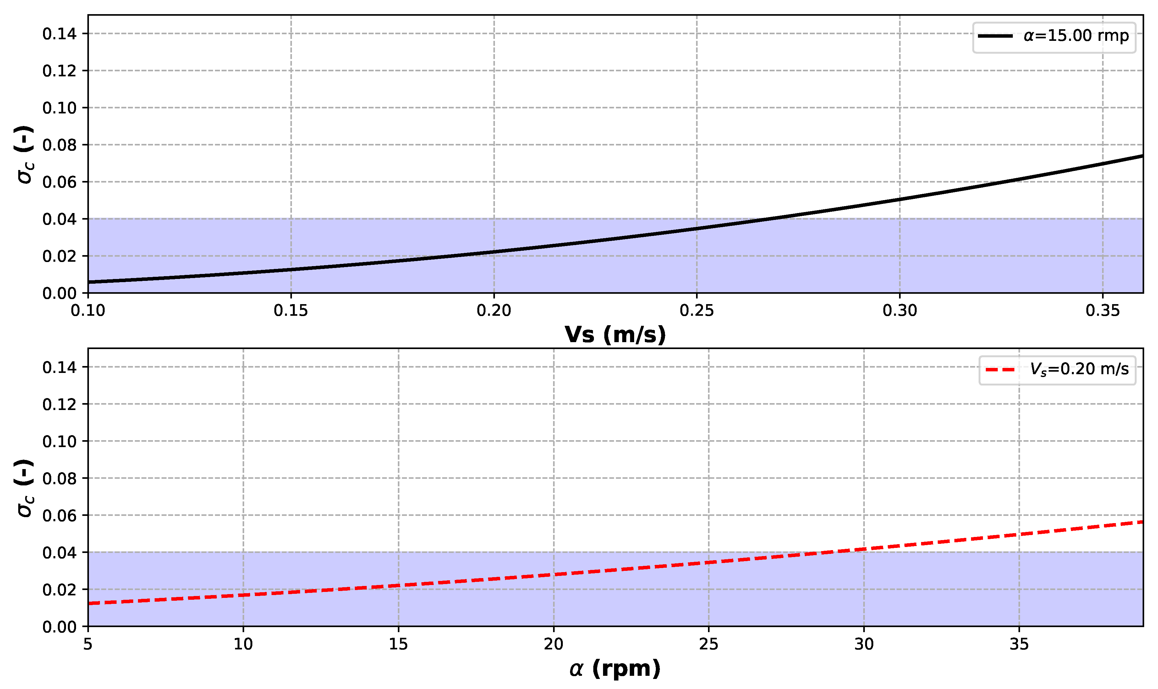0.00–0.05). It has to be stressed that the definition of the empirical source term fractions may take advantage of either monitoring activities or empirical formulations. Just as an example, Hayes et al. [33] proposed an empirical formulation aimed at estimating the rate of sediment (r) re-suspended by cutterhead dredge as a fraction of sediment mass dredged:

$$r=\frac{{\left(L_c{d}_c\right)}^{1.966}{\left|V_s\pm \pi d_c\alpha \right|}^{1.966}{\left(V_s{A}_E\right)}^{1.804}}{1.099Q^{3.770}},$$

(3)

where r (%) is the fraction of sediment mass dredged expressed as a percentage (hence intimately related to the source term fraction ${\sigma }_c=r/100$), $L_c$ (m) is the length of the cutterhead, $d_c$ (m) is the cutter diameter, $V_s$ (m/s) is the swing velocity, $\alpha$ (rounds per second) is the rotational speed of the cutter, $A_E$ (m${}^2$) is the total surface area exposed to washing, Q (m${}^3/$s) is the volumetric flow rate into the dredge pipe. If overcutting is considered (i.e., the positive sign is used in the numerator of Equation (3)), Figure 3 shows the estimate of the empirical source term fraction ${\sigma }_c$ for varying swing velocity ($V_s$) and varying rotation speed of the cutter ($\alpha$) for a typical 16-in. (0.41 m) dredge (e.g., [33], $d_c=1.07$ m, $L_c=0.91$ m, $A_E\simeq 1.3$ m${}^2$). It could be observed that the empirical source term fraction proposed by Becker et al. [8] (dashed areas in Figure 3) is of the same order of magnitude given by the more detailed empirical formulation by Hayes et al. [33].

It has to be noticed that Equation (2) gives the mass of fine sediments available to the far field. In order to get the correct estimate of the source term, a sediment flux should be provided. Then, Becker et al. [8] suggest to simply divide the mass $m_r$ by the time duration of the considered phase (i.e., either excavation, transport, or disposal). This highlights the importance of the analysis of the work phases. This is equally crucial when dealing with the timing and the location of the source term within the computational domain (see Section 5, Figure 4 and Figure 5). Indeed, depending on the operational parameters of the handling works, the source term can be described by either a time-varying or constant intensity and by either a time-varying or fixed location. On the other hand, depending on the spatial resolution of the study, the source term can be described by either a punctual or a finite extent re-suspension source.

Figure 4 aims at synthesizing the main features of the source term estimation and how it can be applied to the computational domain.

5. Preliminary Information and Modeling Phases

The modeling approach has to be feasible both from the controlling authorities point of view, that need reliable results to avoid, or at least to minimize, detrimental effects on the environment, and from the contractors point of view that have to pay attention to the economic and technical feasibility of the work.

Within the framework of the preliminary information phase, the preliminary analysis should be devoted to identifying the need of more detailed studies to prevent and/or mitigate the expected environmental effects.

The first and more basic preliminary studies are based on the retrieval and analyses of known data about environmental forcing (i.e., mainly related to hydrodynamics) along with the physical features of handled sediments (i.e., fine fraction). This approach allows gaining insight into the big picture of the phenomena at hand by identifying potential environmental effects. Environmental issues have to be identified within the frame of a holistic approach, hence by engaging scientists with different expertise (e.g., [38]). Of course, this phase has strong limitations and needs a more detailed analysis if significant environmental effects are expected to occur. In this way, the probability of detrimental environmental effects identified within the preliminary information phase may be confirmed. If this is the case, a second (and deeper) level of modeling to get reliable expectation in terms of turbidity plume evolution and deposition rate distribution at and around the work site should be then performed.

When preliminary modeling phase is concerned, the synthetic scenarios approach is considered the proper candidate to provide fast results. Despite their limitations, analytical models can be used to provide modeling results taking into account the main features of the phenomenon with low computational costs. The solutions of the (simplified) governing equations are typically given in closed-form (they require simple arithmetic operations) or integral-form (they require standard numerical integration techniques). Simplified models for sediment transport and deposition rate estimates often rely on the solution of the two-dimensional advection and diffusion equation of the re-suspended sediments that reads as follow (e.g., [39]):

$$\frac{\partial C}{\partial t}+U\frac{\partial C}{\partial x}+V\frac{\partial C}{\partial y}+\frac{\partial }{\partial x}\left(D_x\frac{\partial C}{\partial x}\right)+\frac{\partial }{\partial y}\left(D_y\frac{\partial C}{\partial y}\right)=q-\frac{w_s}{h}C,$$

(4)

where x and y are the horizontal coordinates; t is the elapsed time; C is the depth-averaged sediments concentration (intimately related to the SSC); U and V are the x- and y-component of the ambient current respectively; $D_x$ and $D_y$ are the diffusion coefficients; $w_s$ is the settling velocity; h is the water depth; q is the source term, often referred to as re-suspension source strength (e.g., [6]). The latter is intended to describe the sediments actually available to the far-field passive transport (see Section 4). Equation (4) neglects the vertical variability of SSC. These models also consider homogeneous environmental currents (i.e., not variable in space), even if variable over time, homogeneous and constant diffusion coefficients (albeit with the possibility of simulating anisotropy of the medium and of the flow), constant depth and constant settling velocity. It is therefore clear that these models can only be used within the preliminary modeling phase, in which simplified models can in any case describe salient features of the spatial and temporal evolution of the plume, and thus highlight when environmental critical issues can potentially occur.

As far as the source term is concerned, analytical models are usually able to evaluate the evolution of the turbidity plume with a constant production of sediments over time located in a fixed area (often referred to as continuous source, e.g., [40,41]). Nevertheless, analytical models can take into account the variation, in both time and space, of location and strength of the re-suspension source during the work progression (e.g., [39]). Thus, it is possible to provide the temporal and spatial picture of the resulting plume evolution. Figure 5 shows a typical example obtained by using the analytical approach proposed by Di Risio et al. ([39]) in the case of dredging activities performed with a hydraulic dredge and a mechanical dredge. In the former case (left panel), the re-suspension is modeled as a moving and continuous source with varying intensity. In the latter (right panel), the re-suspension is modeled as a moving and intermittent source.

Even with their strong limitations, analytical models were demonstrated to be able for describing the big picture of the phenomenon at hand [39] and for the comparison of the effects for different scenarios. Therefore, they can be used to address the general environmental questions, allowing a first rough estimation of the maximum impacted area. Indeed, this is useful to guide more detailed numerical analysis and to select the more appropriate simulation scenarios in terms of both environmental forcing and operational techniques.

6. Detailed Modeling Phase

6.1. Hydrodynamic Modeling

Within the detailed modeling phase, hydrodynamics plays a crucial role. The selection of the models type and the accuracy levels of the modeling scenarios should be representative of the project-specific features and of the spatial and temporal scales of the main physical processes driving the sediment transport phenomena. Then, the analysis has to be based on the environmental conditions of the intervention site: the complexity of the models implies the knowledge about forcing terms and the geometry of the site.

Basically, the hydrodynamic modeling is aimed at estimating the kinematic field (i.e., water levels and currents) responsible for the plume dispersion into the computational domain. The system of governing equations is rather complex and solved by numerical models with a high computational cost. This allows the study of very small spatial domains and for short-duration time windows. To overcome this limitation some simplifications are needed. These simplifications modify the governing equations (and therefore the processes that they are able to reproduce) to allow the analysis of larger areas and for longer time windows. In order to simplify the equations, it is important to identify the crucial key factors forcing the hydrodynamics. Just as an example, wave action plays a key role in the re-suspension and dispersion of sediments in relatively shallow water, while it can be intended as a secondary factor in deep water, where stratified phenomena must be taken into account instead. Indeed, waves and currents interact and influence each other (wave-current interaction). The presence of wave motion generates alterations in the hydrodynamic field that are almost negligible offshore, but may become significant in coastal areas. Even in transitional environments, usually characterized by shallow depths and mainly influenced by tidal oscillations, the action of wind waves produces hydrodynamic effects (and consequently transport phenomena due to interaction with the seabed) that are often not negligible. In turn, also the currents field can generate variations on the wave field (i.e., refraction). This phenomenon may become of great importance in areas such as transition environments characterized by the presence of river mouths or coastal areas characterized by the presence of intense local currents (e.g., rip currents, [42]).

Based on the selected driving forces, short wave propagation and long waves effects may be solved within either a coupled or uncoupled approach. Based on the importance of flow stratification, either two- (2DH), three- (3D), quasi-three-dimensional (Q3D) or multilayer models have to be considered.

Table 2. Applicability of model type for a series of relevant cases, when model type as well as computational costs are accounted for. (++) suitable (even considering computational load with respect to expected results); (+): possible; (o): not completely suitable, hence the results may be affected by the model formulation; (-): not suitable, hence the results are strongly affected by the model formulation.

Case	Model Type
	3D, Q3D, Multilayer	2DH
Shallow water dredging	(+)	(++)
Intermediate to deep water dredging	(++)	(-)
Dredging with re-suspension localized at the bottom	(++)	(-)
Dredging with homogeneous (along the water column) re-suspension	(+)	(++)
Disposal in coastal areas	(+)	(++)
Disposal in semi-enclosed basins with negligible flow stratification	(+)	(++)
Disposal in semi-enclosed basins with relevant wind action	(++)	(+)
Disposal in transitional areas	(++)	(o)
Disposal in transitional areas with significant stratification	(++)	(-)
Disposal in offshore areas	(++)	(o)

synthesizes the applicability of the considered model types for a series of relevant cases within the frame of the mathematical modeling of physical effects induced by marine sediments handling works.

When wave propagation is addressed as a main driving force, the coupled approach aims at describing wave propagation by obtaining a detailed description of its time and spatial propagation. On the other hand, the coupling may be carried out by using the numerical results obtained by a wave propagation model as the forcing term of a hydrodynamic model able to give currents and water levels on a time scale longer than the short-waves period (and vice versa when the effects of currents on the wave propagation have to be considered).

3D numerical models are based on the resolutions of approximated equations solved in the three-dimensional space. The approximations (e.g., Reynolds Averaged Navier Stokes (RANS), large eddy simulation (LES)) are needed to make the numerical models usable within the frame of reasonably large domains. Nevertheless, they are characterized by large computational costs and then they are appropriate only when extremely detailed studies are needed. Examples of these models are NEMO (e.g., [43]), MOHID (e.g., [44]), ADCIRC (e.g., [45]), MIKE3 (e.g., [46]).

On the other hand, 2DH, quasi-3D (Q3D), and multi-layer models are based on equations integrated along the vertical direction. The use of 2DH models is appropriate when dealing with marine-coastal environments in which the vertical dimension of the domain, i.e., the water depth, is significantly smaller than the horizontal dimension (e.g., coastal and transition areas). However, it is necessary to pay attention to the applications for which the effects of vertical processes are important, such as stratified flows (e.g., river mouths with fresh water inlet in a salty environment) or wind driven circulation that can be characterized by high variations of the current profiles along the vertical direction. In such cases, it is possible to use models that, although not strictly three-dimensional, maintain information on the vertical variability of the quantities of interest (e.g., [47]). One approach is to hypothesize a given structure of the variability of quantities along the depth (Q3D models). Alternatively, it is possible to use several layers to integrate the governing equations by taking into account the flow stratification (multi-layer models). Examples of such a kind of models are SHORECIRC (e.g., [48]), DELFT3D-FLOW (e.g., [49]), MIKE21 (e.g., [50]), SHYFEM (e.g., [51]), POM (e.g., [52]), ROMS (e.g., [53]), SWASH (e.g., [54]), XBeach (e.g., [55]).

It has to be underlined that the hydrodynamic studies, i.e., the estimate of water levels and currents, need to take into account several driving forces in the computational domain and at the boundaries. The former, with different relevance depending on the area of application of the analysis (coastal and transitional areas, semi-closed basins, offshore areas), is made up of: wind and wave action, tidal oscillations, inlets characterized by different densities (e.g., river mouths or industrial discharges) for which it is necessary to take into account the buoyancy effects. The latter, on the other hand, consists of large-scale forcing, such as tidal induced currents and basin oscillations (e.g., wind setup, seiches).

The model must also take into account the physical processes related to the interaction of hydrodynamics with the boundaries of the area of interest (e.g., the sea bottom, the coastline and the open boundaries) as well as any elements placed within the calculation domain (e.g., coastal defenses, intertidal morphological structures in lagoon environments, bars or shafts in mouth areas, offshore structures if detectable by the resolution used in the model).

6.2. Sediment Transport and Deposition Modeling

Models for transport phenomena (dispersion, diffusion, and deposition) require the knowledge of the hydrodynamic field and the characteristics of the source term in order to produce reliable estimates of the spatial and temporal variability of suspended sediments (and of any associated contamination).

Numerical models for transport phenomena of suspended sediments are mainly distinguished in Eulerian and Lagrangian models on the basis of the selected approach to define the governing equation.

The Eulerian approach follows a formulation based on the description of the sediment concentration point by point, as given in Section 5 by Equation (4) in the special case of a two-dimensional approach. The resolution of the advection–diffusion equation allows for evaluating the space–time evolution of the SSC as a function of the hydrodynamic field and of the specific features of the source term. Similarly to hydrodynamic models, the governing equations can be simplified by averaging on small temporal or spatial scales (RANS and LES) by introducing parameters that represent the turbulence.

The Lagrangian method is based on a formulation that follows the spatial and temporal evolution of the position of individual particles, each representing a portion of the sediment plume. The main peculiarity of the mathematical formulation is that the effect of turbulence is represented by a stochastic formulation modeled by the random vector $\overrightarrow{d_h}$ (random walk models). As an example, the two-dimensional governing equation in the finite difference framework provided in [5,56] reads as follows:

$$\overrightarrow{r}\left(t+\delta t\right)=\overrightarrow{r}\left(t\right)+\delta t\left(\overrightarrow{v}+\sqrt{\frac{6k_h}{\delta t}}\overrightarrow{d_h}\right),$$

(5)

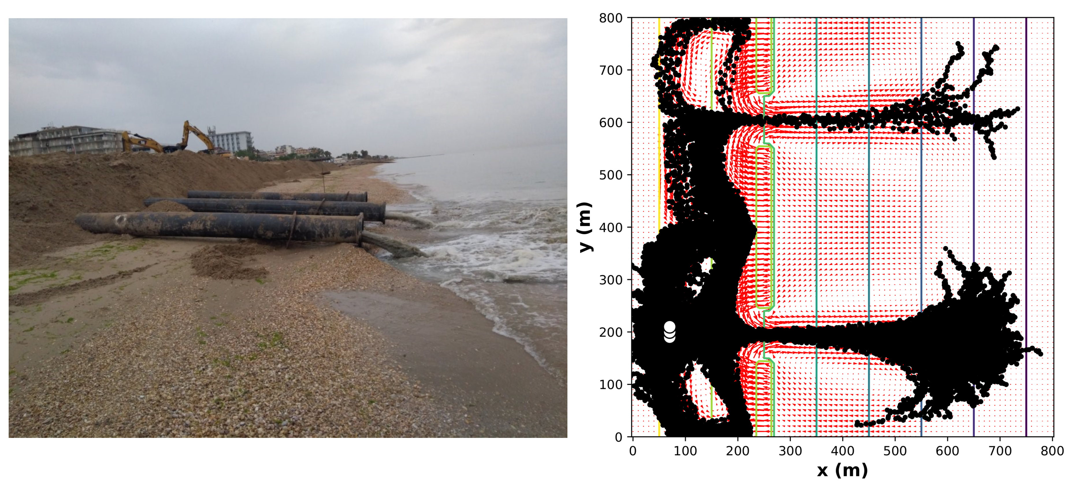
where $\overrightarrow{r}$ is the position vector of a specific individual particle, $\delta t$ is the time step, $\overrightarrow{v}$ is the (horizontal) current field, $k_h$ is the horizontal eddy diffusivity, and $\overrightarrow{d_h}$ is a vector with dimensionless components uniformly distributed in the range $\left[-1,+1\right]$. As an example, Figure 6 shows the particles dispersion due to the nearshore disposal during a beach nourishment intervention estimated by means of a random walk model.

The use of Equation (5) is based on the hypothesis that the sediment is a passive tracer, i.e., it does not alter hydrodynamics, but is simply advected by the current field and progressively dispersed in the water column. The higher the sediment concentration, the lower the validity of this hypothesis, since the rheological behavior of the sediment-water mixture varies. As a consequence, this approximation is likely to be more acceptable in the far field than close to the sediment release source. The use of this hypothesis makes it possible to describe the sediment diffusion and transport process, decoupled from the hydrodynamic model. Alternatively, this aspect can be taken into consideration by altering the local value of the fluid density (also dependent on temperature and salinity). Considering that density also affects the hydrodynamic equations, it is then necessary to solve in a coupled way the two systems of equations (hydrodynamics and transport/diffusion). Many numerical models for hydrodynamics simulation include specific modules (Eulerian and/or Lagrangian) for sediment transport (e.g., [44,57,58]).

In order to improve the accuracy of the solutions, it is possible to consider different granulometric classes. In this case it is necessary to solve the equations separately for each class. In particular, this approach is useful to separate and better reproduce the dynamics of the finest fraction of sediment that undergoes transport processes in larger areas.

As far as DEP is concerned, there are many formulations available in the literature (e.g., [59,60,61,62,63,64]). For the deposition of non-cohesive sediments, it is possible to refer to the formulation proposed by Stokes, based on the assumption that the flow is in a viscous regime. However, when dealing with cohesive sediment it tends to underestimate deposition (and consequently to overestimate SSC). Therefore, in some cases, it is necessary to resort to formulations that take into account the presence of cohesive sediment (e.g., [65]), which can generate floccules for the attraction between particles that causes aggregation (e.g., [66,67,68]). Flocculation influences not only the effective diameter of the settling particles, but also the density, since floccules have a lower density than sediment particles with the same diameter [69].

Re-suspension of the sediments is an intensively studied problem but is still of interest (e.g., [70]). It is important to underline the differences in the re-suspension process as a function of the sediment characteristics. In fact, the size and density of the particles are the main factors influencing the re-suspension of non-cohesive sediments. Whereas, cohesive sediments, depending on the composition and the cohesion levels, can be grouped in two types: those that tend to aggregate into floccules when re-suspending and those whose re-suspension occurs as a muddy mixture [68]. Furthermore, cohesive and non-cohesive sediments are generally characterized by different consolidation processes. Non-cohesive sediments tend to consolidate rapidly and form a layer characterized by constant erodibility at the same depths. Cohesive sediments, on the contrary, tend to consolidate slowly and form cohesive base layers characterized by variable erodibility over time and depth. Re-suspension of cohesive sediments is mostly studied in the case of unidirectional or slowly variable currents (e.g., tidal currents), although the action of surface waves sometimes plays a significant role. In particular, the fluctuation of pressure values induced by the waves propagation can weaken and fluidize the sediment at the bottom [71,72]. The erodibility can also vary in relation to other physical, chemical and biological factors, such as the mineralogical composition, the presence of interstitial water and the pH, the ionic composition, the quantity and the type of organic matter in the different types of sediment (e.g., [68]).

Biological activity can also cause a temporal and spatial variability of the sediment erodibility (e.g., [73]). Re-suspension formulations are generally based on the comparison between the tangential stress (on the bottom) due to the hydrodynamics and a critical value of the tangential tension beyond which the sediment is re-suspended. This critical value is related to the geotechnical characteristics of the sediment [74,75] and is often assessed on an empirical basis [69].

7. Data Analysis and Representation

Past research works (e.g., [14,21,22,24,26,47,76]) show a lack of tools able to synthesize numerical results for supporting decision-makers in different design and environmental conditions. Maps showing the predicted (e.g., maximum and mean) SSC at different water depths and DEP, as well as time series at different key sites, are recommended to support planning and environmental approval. However, uniform criteria for the analysis and representation of numerical results obtained within preliminary modeling phase and detailed modeling phase have to be defined consistently with the characteristics of the modeling objectives. Indeed, they have to be defined based on the main physical processes identified as of primary interest for the considered environmental context, operational phase and environmental critical issues (if any) in the neighboring of the intervention site. Then, they can be useful also to select modeling scenarios (see Section 3) suitable to assess the fate and transport of the handled sediments with sufficient accuracy for the purpose of impact assessment.

An integrated, flexible and replicable methodological approach for synthesizing parameters related to water quality variations that arise from sediment handling activities is proposed herein starting from the extension of the environmental assessment method for dredging activity (Dr-EAM) methodology proposed by Feola et al. [26] to different environmental context (i.e., off-shore, near-shore and enclosed basin this paper deals with). These evaluations are needed for the assessment of the environmental impacts related to sediment handling projects and, in particular, for the evaluation of the severity of impacts on sensitive environmental receptors.

Based on past research works (e.g., [22,26]), it is recognized the importance of defining reference levels representative of the baseline variability of parameters of interest (e.g., SSC, DEP) before the handling operations or, during the activities, in reference areas potentially not affected by the handling works. A series of multiple reference levels with growing environmental criticality should be used to quantify the significance of the effects related to turbidity plumes during the project execution (e.g., [77]). These (single or multiple) reference levels must be established based on literature, site-specific monitoring and expert judgment depending on the project features (e.g., extension, duration, volume of handled sediments) and the expected interactions with the environmental critical issues (if any).

The source–path–receptor model can be used to represent the link between the sediment re-suspension source (intervention site) and the receptor (e.g., [18]). Although beyond the scope of this paper, it is important to stress that for a proper correlation between the significance of physical effects to the severity of possible impacts on the biological compartment, reference levels definition should also consider site-specific receptor tolerance limits (when they are available and/or they can be inferred from specific stress-response curves) to the expected water quality variation during execution. The severity of impacts is related to the presence of the expected and/or detected environmental issues, their location (with respect to sediment source and local currents), their nature and their ecological status (Figure 7).

The evaluation of the significance of effects must necessarily consider different aspects of the induced perturbations to the environmental effects, such as intensity, duration and frequency of events of SSC and DEP increase (e.g., [10,26,78,79,80,81]). The relationship between intensity, duration of perturbation and the related environmental effects on the specific receptor can be derived on the basis of site-specific data, on literature data or by expert judgment. When literature information or field data representative of the study area are not available, the reference levels can be defined using modeling studies in order to perform an analysis of the variability intervals of the parameters of interest. It is important to produce maps that summarize the modeling results [14]. Following the indications proposed by Feola et al. [26], a flexible, consistent and integrated methodological approach is presented in terms of standard and easily replicable techniques. The approach is suitable to support the identification and an easy assessment of the magnitude of potential effects in relation to intensity, duration and frequency of deviations from identified reference levels. In particular, it is useful to define a discrete number of check-points for extracting time series of output parameters throughout the whole period of simulation. Check-points have to be regularly distributed in the domain with a spatial scale chosen as a function of the spatial variability of the numerical results. For each check-point, time series can be extracted at different depths in the water column and at the seabed then analyzed and combined to derive suitable statistical parameters and indexes related to intensity, duration, and magnitude of exceedance of reference levels. Maps representing these parameters allow direct comparison of effects due to sediment handling works activity at progressive distances from the re-suspension zone. If the selected parameter is of hydrodynamic type, it will be possible to identify, for each scenario on both a seasonal and annual basis, zones with a different agitation level, as it will be possible to represent the spatial variability of the dispersion and deposition of the turbidity plume as SSC in water column and DEP at the bottom. To account for the combined effect of different parameters (e.g., duration and intensity), that cannot describe the significance of the exceedance of the reference level if separately considered, different methodological approaches can be used.

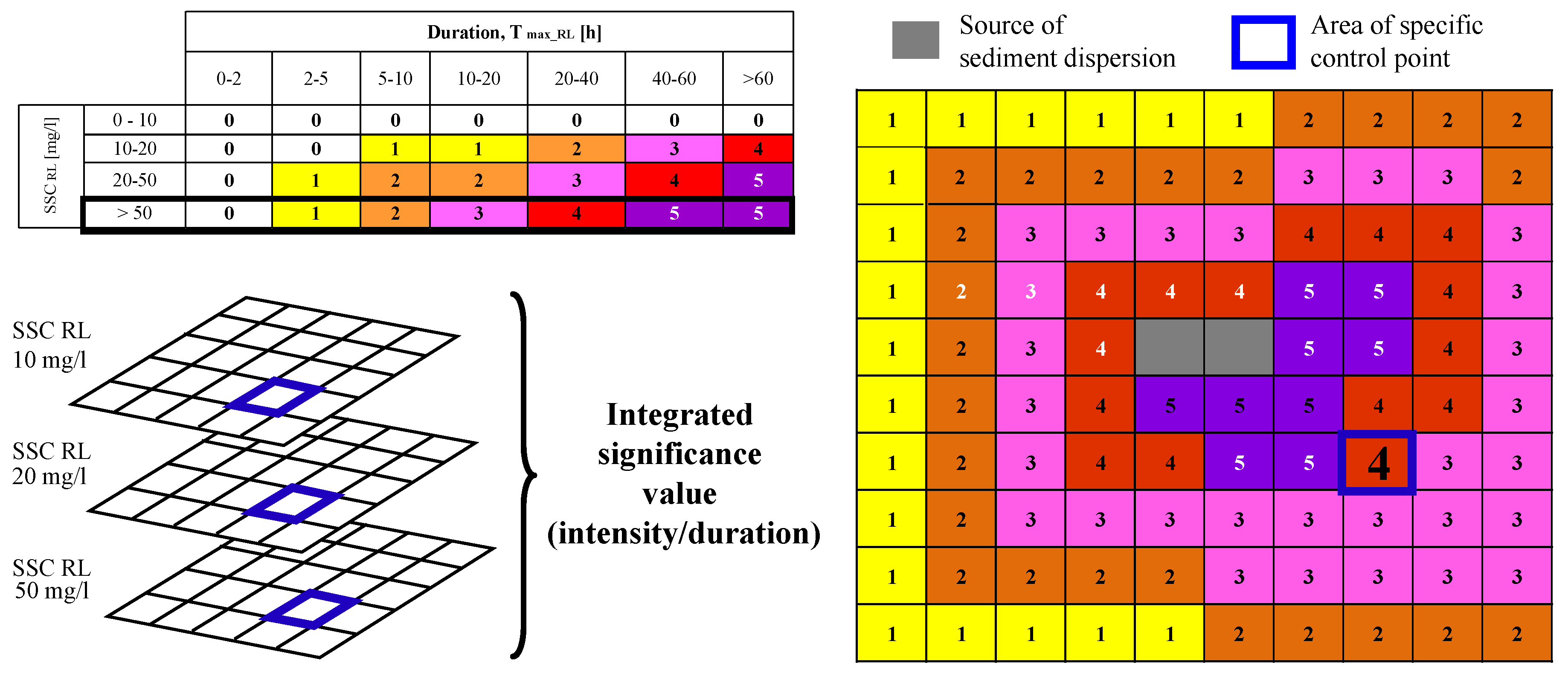
A first approach for the definition of the significance of physical effects involves the use of a series of reference levels, the exceedance of which leads to the identification of intensities and durations. As an example, Figure 8 shows some indicative reference levels for intensity (SSC${}_{RL}$) and duration intervals (T${}_{max\_RL}$), i.e., the maximum duration of time windows during which SSC exceeds the specific SSC${}_{RL}$. The significance of the environmental effects is then defined in terms of a combination of SSC${}_{RL}$ and T${}_{max\_RL}$. Of course, the same method may be performed by changing the reference levels as a function of the specific receptor or by using other pairs of meaningful parameters (e.g., frequency of occurrence, [78]) on the basis of project-specific and/or site-specific and/or receptor-specific evaluations. In particular, synthetic maps are defined for each reference level in terms of intensity (e.g., SSC${}_{RL}$ = 10, 20, 50 mg/L in the example shown in Figure 8) storing at the single control point the significance value of the effect associated with the maximum duration of uninterrupted persistence of SSC above the specific value. From the overlap of the maps, the maximum value of registered significance is obtained for each specific control point. Maps can be overlapped to the location of sensitive habitats and ecological receptors in order to relate the sediment plume dynamic with different targets.

A second approach involves the use of a single index. Feola et al. [26] proposed to use the SSC number (SSC${}_{num}$; mg s/L, e.g., [82]) that gives integral information about intensity, duration and frequency of exceedance of reference level. Basically, it is defined, for each simulation scenario (i), as the sum of the products of the mean intensity above reference level (SSC${}_{mean\_RL,i}$) and the related duration ($t_j$, $j=1\dots M_i$, with $M_i$ the number of the considered events). Then, it reads (e.g., [26,82,83]):

$$SS{C}_{num,i}=\sum _{j=1}^{M_i}SS{C}_{mean\_RL,i}{t}_j$$

(6)

where SSC${}_{num,i}$ is the SSC number related to the specific i-th scenario. Maps of this integrated index can be then evaluated by analyzing the time series for each control point and for different values of the reference level.

Further useful analysis should be suitable to quantify the spatial and temporal variability of the effects associated with the dispersion of the turbidity plumes as a function of the distance from the sediment source. For these purposes semi-variograms can be used (e.g., [84]). Basically, the semi-variogram is defined as half of the averaged squared difference of the parameter at hand (SSC in this case) between points located at different distances. Then, the analysis of the semi-variogram allows the direct measurement of the spatial scale of the transport phenomena resulting from the generation of the turbidity plume and can be used to quantitatively compare the extent of the areas affected by the sediment handling activities (influence zone) related to different scenarios of simulation. The use of the semi-variogram provides the estimate of the variance (alteration with respect to the undisturbed value) of the parameter at hand modeled as a stochastic variable, and the estimate of the physical intensity of the alterations with respect to the undisturbed value.

8. The Role of Monitoring

8.1. Modeling and Monitoring Feedback System

Modeling–monitoring interactions are often recommended in environmental impact assessment procedures (and other regulatory frameworks) for assessing the compliance of selected operational criteria with the established environmental requirements. Basically, the selection of the modeling accuracy, and of the type of data to be collected as well, heavily depends on the general requirements of the various monitoring phases (before, during and after execution monitoring, e.g., [18]), and on the short- and long-term effects to be verified. Different types of data must be collected for determining the dynamics and the composition of turbidity plumes. The most common parameters needed to validate models are: sedimentological, meteo–climatic, hydrodynamic, water quality, topo–bathymetric and descriptive (e.g., coastline features, the presence of infrastructures or specific land-uses) data. The objective of measuring physical parameters not directly related to water quality (e.g., currents, waves, water elevations) is to provide information on how long a plume can remain in a particular area and on the time required for its dispersion to adjacent waters, as well as considering factors that may increase turbulence in the water column causing additional turbidity and preventing sedimentation.

In order to optimize a modeling–monitoring feedback system, typical environmental questions to be answered in the early preliminary planning phases are: (i) what types of sediment spill sources could be expected/distinguished (e.g., single point-spill event, continuous point-spill over a certain period); (ii) whether suspended sediments will leave the dredge- or dump-site; (iii) where the material will go and how much material will remain in the water column after a certain time. The most used parameter to characterize sediment plumes is turbidity, calibrated with in situ total suspended solids measures (TSS), defined as the total mass of material in a given volume of water, in mg/L. Nonetheless, establishing a reliable relationship between TSS and turbidity is not always possible because of the variation in characteristics of the suspended material. For defining turbidity values three aspects are usually considered: (i) turbidity level in the dredging area; (ii) the horizontal dispersion of the sediment cloud (for different hydrodynamics conditions); (iii) the settling time of the sediment cloud after cessation of operations. According to Pennekamp et al. [32], monitoring results allow the evaluations of the depth-averaged background concentration, of the characteristic increase of depth-averaged concentration at different distance from dredging/disposal activity, of the decay time of the re-suspended sediment after the execution of handling operations after which the turbidity return to background values, of the source term. In addition, chemical-physical parameters (temperature, salinity, conductivity and density conditions) are important to identify when sediment plumes significantly differ from the surrounding water. Dissolved oxygen and pH are commonly measured as indicators of water quality and of potential impact on biological resources (e.g., re-suspension of anoxic sediments may lower dissolved oxygen concentrations in the water column).

Fixed stations are required for comprehensive and regular monitoring over time. In fact, continuous time-series (single point or profiler) provide valuable information on the temporal variability of the monitoring variables along the water column. In particular, fixed stations allow collecting the background conditions during different environmental conditions before the execution of the works and to verify the selected reference levels during their execution.

During the execution phase, both fixed and mobile monitoring stations are required. Mobile stations (e.g., samplings from a vessel) are required when measurements at various locations over short-periods of time are needed, to one or more water depths, and to track the near-field plume through the water column. These types of measurements allows us to follow any change of the operational techniques that could influence sediment spill concentrations. Sampling time can be significantly increased depending both on site conditions (e.g., water depth and rate at which hydrodynamic conditions can vary) and on the purpose of the monitoring project phases.

The selection of the monitoring tools (i.e., fixed platforms, vessels, or towed vertical profilers) and of the sampling techniques is important to maximize the usefulness of the modeling–monitoring feedback system within the different phases of the project. Thus, understanding the advantages and limitations of the various available sampling techniques is important to determine the most cost-effective approach for sediment plumes monitoring. In general, using multiple instruments on the same platform reduces sampling time and provides synoptic measurements of the parameters being measured.

Based on the results of the monitoring and modeling analysis, it is possible to deepen the understanding of the system and its responses to pressures induced by changes on the involved environmental variables (chemical-physical and biological). Then it is possible to modify the design and monitoring choices. Mathematical models allow hydrodynamic and sediment transport evaluations (in time and space) for different selected spill scenarios, supporting the optimization of both work plans and environmental monitoring programs in the different project phases taking into account operational and environmental aspects. Monitoring data, on the other hand, are crucial to define input for near-field and far-field models, as well as for their calibration and validation and to verify the reliability of the modeling simplifications and results. For efficient management of sediment handling works, the modeling–monitoring feedback system is recommended herein as part of the proposed integrated modeling approach. The main relationships between modeling and monitoring activities and the main details on various deployment platforms for data collection (fixed platforms, vessels, or towed vertical profilers) at different stages of project design are highlighted in the followings.

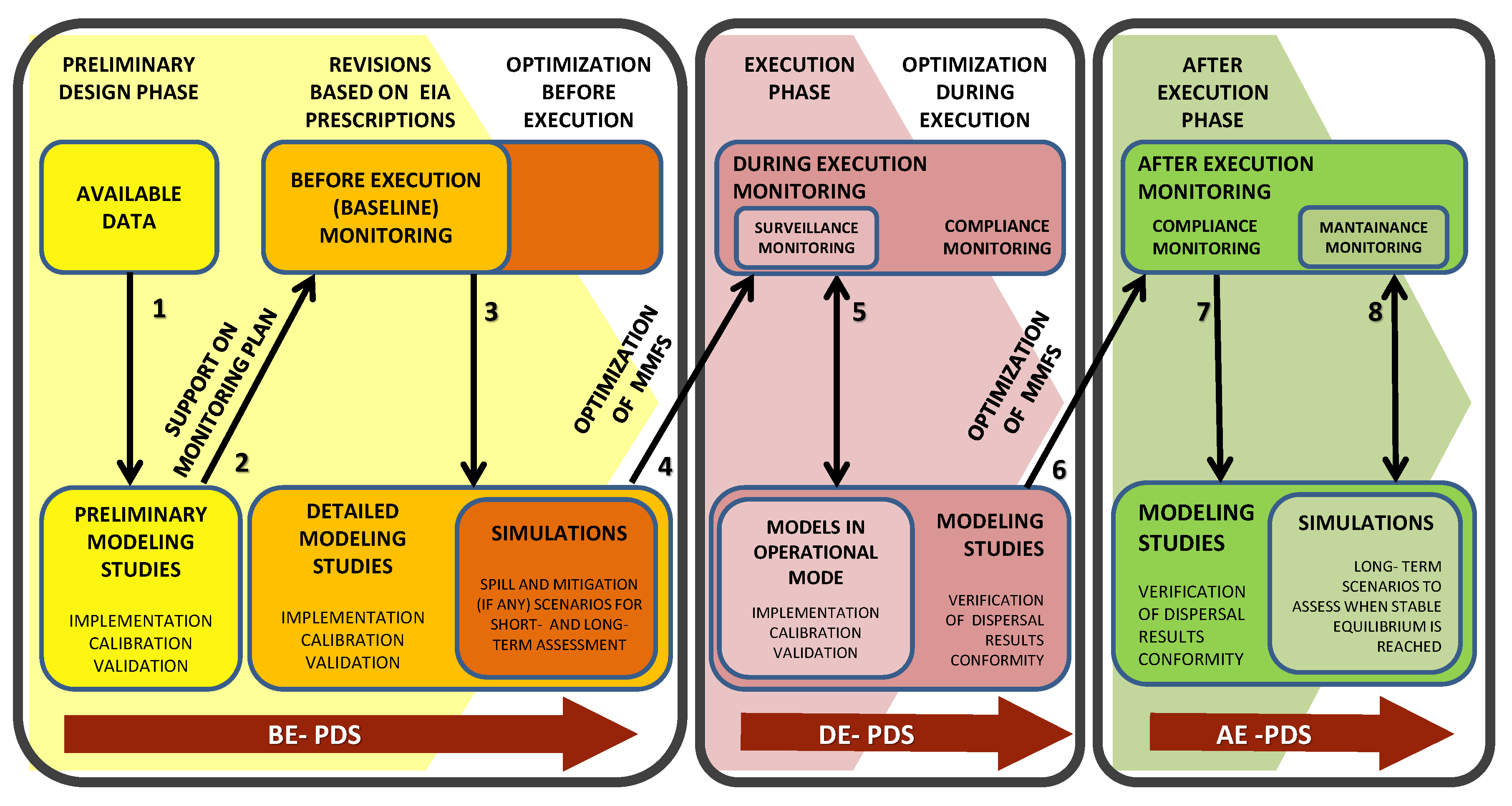
Figure 9 shows the main interactions within the modeling–monitoring feedback system that should be carried out to verify the feasibility and the environmental compatibility of interventions in various design, execution and monitoring phases (i.e., before, during and after execution). In the preliminary design phase (i.e., before works execution), the modeling–monitoring feedback system serves as a supporting tool for the approval of work plans and for designing of suitable monitoring programs. In this context, the feedback between preliminary modeling spill scenarios and baseline-monitoring allows the selection of background conditions not related to the works execution. In particular, the determination of statistically reliable reference levels for the selected variables (e.g., SSC, DEP) will allow, during execution, to analyze monitoring and modeling results and to evaluate whether mitigation actions should be taken. Indeed, in the early stages of monitoring planning, site-specific information on types, distances and status of any sensitive objectives and receptors is needed for relating the significance of effects in terms of physical changes to the severity of impacts on critical targets (see Section 7).

In fact, during and after sediment handling works, the modeling–monitoring feedback system is useful to verify (in the short-term) the fulfillment of the selected operational criteria and (in the short- and long-term) the compliance with the requirements of environmental protection mechanisms including legislation, contractor conditions and sustainability protocols [18]. In particular, changes of selected variables (e.g., SSC) can be compared with the selected (single or multiple) site-specific reference levels for water quality. For the short-term assessment, the surveillance monitoring is performed in the execution phase, trough the combined use of fixed and mobile (on-vessel) monitoring stations (see VBKO [85] and Aarninkhof et al. [86] for more details). This provides extensive sediment flux data useful for early warning to ensure that the amount of sediment re-suspension and dispersion is kept below the site-specific reference levels. Moreover, field data are crucial to validate the models to reduce the modeling uncertainties (i.e., the estimation of source terms). In addition, increasing knowledge on operational factors used to perform the sediment handling operations (e.g., more details on time schedule, production rate and type of dredges) should be considered for the set-up of more detailed modeling studies and for periodic reviewing of monitoring programs [17].

For interventions of considerable extension or in presence of very sensitive environmental critical issues (e.g., handling of pollutant sediments), the implementation of models in operational mode is useful to handle (mitigate or prevent) critical conditions that may occur during works execution (e.g., time windows of adverse weather and sea conditions, distribution of sediment concentration and sedimentation rates caused by natural or anthropogenic actions). In particular, the use of models in operational mode is recommended, as support to contractors and controlling authorities to promptly adopt proper alert procedures (e.g., interruption or modification of operations, implementations of mitigation measures) selected within a short term operation plan (STOP) aimed at ensuring that key parameters remain below specified alert levels (in term of both intensity and duration of exceedance), when these are forecast in one or more target points.

For the long-term assessment, a comprehensive and regular monitoring must be performed by means of fixed stations, including both the area involved by dispersal of re-suspended or spilled sediments and one or more periodic control points located in undisturbed areas (identified in advance trough the numerical modeling activities) and near environmental sensitive areas (if present). In this case, long-term scenarios should be implemented to forecast long-term effects and then verified through field measurements after the completion of the sediment handling operations. In particular, for a proper management plan, after works execution, monitoring should be performed until undisturbed conditions or a new stable equilibrium of the marine ecosystem (based on environmental considerations and criteria provided by controlling authorities) are achieved.

8.2. Management of Monitoring Data and Information Flow

According to the Adaptive Management approach (e.g., [7,17,87]), a sharing process between the contractor and the authority regarding the modeling–monitoring feedback system (to be foreseen before, during and after the conclusion of detailed studies) is desirable. The sharing process should include standard decision-making procedures and should be functional to optimize the work plan, the mitigation procedures (such as, modifications of dredging schedules, decrease of spill and overflow using special return pipes, closed grabs or clamshells, silt curtains or screens around dredgers) and the monitoring program (number, location and sampling frequency of the stations).

Moreover, within a modeling–monitoring feedback system, the implementation of an environmental information management system (EIMS) is encouraged to constantly enrich the available and usable data-set for a better application of the proposed integrated modeling approach (before, during and after each design and monitoring phases). In particular, project data sheets (PDSs) are promoted for a systematic collection and adequate dissemination of environmental (e.g., climatic an hydrodynamic conditions) and operational data (e.g., details on dredging equipment and techniques, production rate, work time schedules, type and operating mode of any mitigation measures) to be organized in a specific standardized, homogeneous and easily manageable format. This is in order to maximize the usefulness of monitoring data within the various design phases of the same project and to support the initial phases of future projects characterized by similar environmental and operating conditions. Indeed, the availability of data can be useful to increase the reliability of the modeling hypotheses, in particular for the estimation of source term. Information sheets can be considered as guides for data collection. In order to maximize the usefulness of PDSs their compilations should be performed with a frequency suitable to represent the natural background turbidity (e.g., for representative weather and sea conditions, vessel traffic). During the works, it is desirable to compile them also when operational parameters and site-specific environmental conditions change. In particular, the use of standard methodologies for the compilation of project data sheets before execution (BE-PDS), during execution (DE-PDS) and after execution (AE-PDS) phases (see Figure 9) will allow a good efficiency for calibration and validation processes and reliability of the obtained modeling results.

9. Concluding Remarks

This paper deals with the mathematical modeling needed to assess the physical effects induced by sediment handling operations in marine and coastal areas. In particular, it aims at:

• proposing an organic and comprehensive framework about the physical effects induced by sediments handling operations;
• detailing a broad-spectrum modeling approach intended to support contractors and controlling authorities in planning and managing sediment handling operations;
• illustrating an integrated, flexible and replicable methodological approach for synthesizing numerical results;
• highlighting the main features of the required modeling–monitoring feedback system.

The proposed integrated modeling approach for simulating sediment dispersion is intended as a flexible framework to estimate sediment dispersion due to marine sediment handling operations. It has been developed to assess the spatial and temporal variability of suspended sediment concentration and deposition rate by means of hydrodynamic, sediment source and transport models implementation. Different levels of accuracy are suggested for different project and operational phases based on the presence of environmentally sensitive critical issues (if any) and the classification of specific environmental contexts: coastal areas, semi-enclosed basins and offshore areas. In particular, paying attention to the feasibility of the modeling studies, it is proposed to perform a series of analyses with increasing details. Then, detailed (and computational onerous) simulations are suggested only if critical issues are likely to arise based on preliminary information and modeling phases. In order to guide the readers in all the steps of the proposed methodology, a further paper dealing with a series of case studies is in preparation.

One of the main uncertainties in the proposed integrated modeling approach implementation is related to the sediment source estimation. Indeed, site-specific data are required to obtain accurate estimate for release/sedimentation fluxes related to excavation, loads and dumping phases. Here the combined use of in situ data and numerical results is claimed to be powerful. Whereas the numerical results represent the variability of suspended sediment concentration at different time-scale far from the intervention site with acceptable reliability, in situ data are needed to gain insight on detailed aspects of the processes that influence its variability along the horizontal and vertical directions. Specific measurement and monitoring campaigns are among the challenges for giving more accurate model results. Then, the modeling–monitoring feedback system is proposed to be well suited as a framework to support the modeling practice, both with respect to the model and the data requirements. As part of the proposed modeling approach, it contributes to an integrated and application-oriented use of models and observations to monitor physical processes in different project phases (also in operational setting). Moreover, within a modeling–monitoring feedback system, the implementation of an environmental information management system and the compilation of project data sheets are promoted for a better application of the proposed integrated approach approach (before, during and after each design and monitoring phases). In particular, project data sheets compilation is encouraged to constantly enrich the available dataset and to maximize the usefulness of field data acquired during the various design phases of the project to be monitored and to support the initial phases of future projects characterized by similar environmental and operating conditions.