Morphodynamic Acceleration Techniques for Multi-Timescale Predictions of Complex Sandy Interventions

Abstract

Thirty one percent (31%) of the world’s coastline consists of sandy beaches and dunes that form a natural defense protecting the hinterland from flooding. A common measure to mitigate erosion along sandy beaches is the implementation of sand nourishments. The design and acceptance of such a mitigating measure require information on the expected evolution at time scales from storms to decades. Process-based morphodynamic models are increasingly applied, together with morphodynamic acceleration techniques, to obtain detailed information on this wide scale of ranges. This study shows that techniques for the acceleration of the morphological evolution can have a significant impact on the simulated evolution and dispersion of sandy interventions. A calibrated Delft3D model of the Sand Engine mega-nourishment is applied to compare different acceleration techniques, focusing on accuracy and computational times. Results show that acceleration techniques using representative (schematized) wave conditions are not capable of accurately reproducing the morphological response in the first two years. The best reproduction of the morphological behavior of the first five years is obtained by the brute force simulations. Applying input filtering and a compression factor provides similar accuracy yet with a factor five gain in computational cost. An attractive method for the medium to long time scales, which further reduces computational costs, is a method that uses representative wave conditions based on gross longshore transports, while showing similar results as the benchmark simulation. Erosional behavior is captured well in all considered techniques with variations in volumes of about 1 million m${}^3$ after three decades. The spatio-temporal variability of the predicted alongshore and cross-shore distribution of the morphological evolution however have a strong dependency on the selected acceleration technique. A new technique, called ’brute force merged’, which incorporates the full variability of the wave climate, provides the optimal combination of phenomenological accuracy and computational efficiency (a factor of 20 faster than the benchmark brute force technique) at both the short and medium to long time scales. This approach, which combines realistic time series and the mormerge technique, provides an attractive and flexible method to efficiently predict the evolution of complex sandy interventions at time scales from hours to decades.

1. Introduction

Thirty one percent (31%) of the world’s coastline consists of sandy beaches and dunes that form a natural defense protecting the hinterland from flooding [1], at the same time providing valuable space for recreational activities and nature development. Due to alongshore variation in hydraulic loads, sandy shorelines can experience persistent sand losses. In the longer term this may result in a retreat of the shoreline, negatively impacting the functions and values of these areas. To mitigate these effects, coastal managers implement mitigating measures, which can either be hard constructions (e.g., sea wall, revetment) or soft (sandy) strategies comprising sand nourishments.

The design and acceptance of a sandy strategy as a mitigating measure requires sound information on the expected dynamics, both in the short and longer term. Coastal managers base their decisions mostly on medium- to long-term trends (annual to decadal scale) of coastal change. However, extreme episodic events (short-term) can, at times, erode the beach to such an extent that it affects long-term trends of coastal change. Over the event of a storm sudden and large morphological changes may occur [2]. Furthermore, a rapid sequence of storms (“clusters”) may have a different net impact compared to that if the same storms were to occur in the same sequence but with larger gaps in between the individual storms [3,4]. Apart from the event time scale, understanding the interannual and innerannual (seasonal) variability in beach dynamics is also important for coastal management decisions. Especially when it concerns anticipating the possible coastal impacts of a new coastal intervention. This is because the temporal scale of an impact is often interrelated to the spatial scale. While the impacts of larger-scale coastal interventions at sandy coasts might be limited to the local scale in the short-term, these impacts may potentially affect a larger area over time.

For example, the proper design of a port or a mega sand nourishment requires reliable predictions of how the coastal area in the immediate vicinity (∼1 km) of the intervention would respond to it over the first couple of years, as well as how the coastal area farther away from the intervention (∼10 km) might change over a decade or longer. With increasing spatial scales, the potential of inter-dependencies with other (existing) coastal interventions also increases. Thus, impacts manifesting themselves at different spatio-temporal scales, may have profound inter-dependencies as well. Figure 1 illustrates the relevance of different processes over various time and space scales for a mega nourishment and a port development highlighting that for increasing forecast horizons, the number of physical processes that need to be taken into account necessarily increases. Therefore, to robustly predict coastal response to larger scale interventions, a multi spatio-temporal numerical modeling approach is required.

For providing information on the expected long term (i.e., greater than 10 years) coastal behavior, analytical models predicting the sandy shoreline change have proven to be useful in engineering applications for sandy and gravel beaches [5,6,7,8,9]. The inherent simplifications and assumptions result in fast computations, but are limited in predicted output information; e.g., only the shoreline position over time.

Process-based coastal area models have the potential to provide comprehensive information at multiple spatio-temporal scales allowing more detailed evaluation. To date such coastal morphodynamic models are generally able to adequately simulate morphological change due to concurrent tides, waves and currents for short to medium-term time scales; events of 3–4 years [10,11,12,13]. Prediction of the long-term dynamics of sandy interventions have however remained a major challenge for process-based models [14].

At the same time, reducing the computational costs of morphodynamic simulations for coastal areas is a critical issue for engineers [10,15]. To reduce computational costs, for example, mixed method approaches have been studied that combine analytical and process-based models [16]. Even though process-based models of physical systems have greatly benefited from the increasing computational power over the last decades, the use of morphodynamic acceleration techniques is still the only way to perform medium- to long-term morphodynamic predictions [17,18].

In this article, we investigate the performance of multiple acceleration methods applied to multi-timescale morphodynamic forecasts for a sandy coast with respect to accuracy and computational effort. Section 2 summarizes the different morphodynamic acceleration techniques used in this study. The case study, general model setup and validation is presented in Section 3. The details of the acceleration techniques, as applied to the case study, are presented in Section 4. Section 5 presents a verification of the techniques for short and medium-term morphodynamic evolution and discusses phenomenological accuracy and computational effort associated with the different acceleration techniques. Section 6 addresses the results for the different acceleration techniques at decadal time scales, while the conclusions are presented in Section 7.

2. Morphodynamic Acceleration Techniques

The most basic approach to morphodynamic modeling uses unfiltered real-time (hereafter referred to as brute force) time series of forcing conditions (see Figure 2a), which is referred to as the brute force technique (BF). Typically, measured time series of water levels (tide and surge), waves, wind and possibly currents are applied to the morphodynamic model [12]. In this technique, no upscaling of the bed level changes takes place.

One of the major issues in long-term modeling is bridging the gap between small-scale hydrodynamic and transport processes and large-scale morphological changes [10,19]. Elegant acceleration methods have been developed for this purpose, such as the morphological acceleration factor introduced by Lesser et al. [20], hereafter referred to as the morfac. With the morfac method, the simulated morphology is accelerated by multiplying the calculated bed changes with a factor equal to the morfac. For example, a simulation over one tidal cycle (12 h) with a morfac of 10 represents 120 h of morphological change. This method is presently one of the most commonly applied acceleration methods [21,22,23,24,25]. With the use of the morfac, in combination with model input reduction techniques discussed in this paper, the time required to perform simulations of morphological changes over time periods of years to decades can be reduced drastically.

Besides the morfac, the reduction of model input is another commonly used acceleration method on the hydrodynamic timescale. Input reduction aims to reduce the computational effort through applying a reduced set of forcing conditions representing a longer-term signal. This can be achieved by ignoring conditions in the brute-force time series that do not contribute to the bed level changes (brute force filtering), or by schematizing the forcing conditions resulting in a set of representative conditions (schematized input reduction). The latter method is commonly applied with morfac larger than one while the former can also be applied with a morfac equal to one (non-scaled).

This study focuses on the evaluation of six morphodynamic acceleration techniques: three using brute force time series and three using representative (schematized) wave conditions. The aforementioned brute force simulation (BF with morfac = 1) is used as the benchmark simulation.

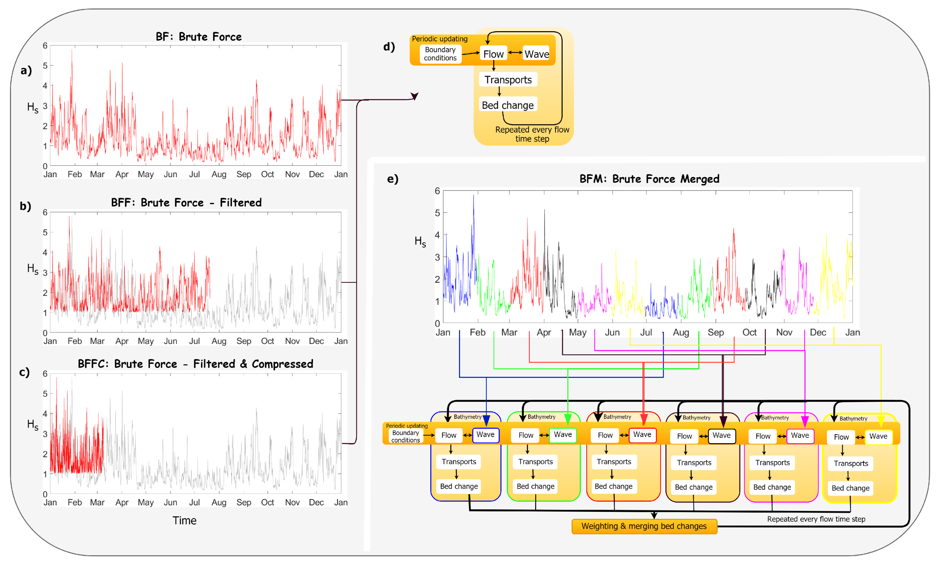
2.1. Techniques Using Brute Force Time Series

2.1.1. Existing Brute Force Techniques

This section discusses the considered techniques to accelerate model results from a hydrodynamic time scale to morphological time scales ranging from days to decades for a wave-dominated coastal domain. The techniques are illustrated in Figure 2 and characteristics are given in Figure 3.

The first acceleration technique involves input reduction by filtering forcing conditions that are relevant to the morphodynamics; referred to as the filtered brute force technique (BFF); see Figure 2b. Analysis of the brute force simulation can reveal which forcing conditions contribute to the morphological evolution. For example, Luijendijk et al. [26] demonstrated that only waves with H${}_s$> 1 m contribute to the evolution of a large-scale nourishment, and omitting the small waves results in a 40% reduction of computational time (compared to the corresponding BF simulation).

A variant to the filtered brute force technique, which combines the input reduction and morphological acceleration factor, is referred to as the compressed, filtered brute force technique (BFFC); see Figure 2c. In this technique the time series of the forcing conditions are compressed with a factor equal to the morfac (> 1) [18]. Time series of the waves, surge and wind can be compressed in this way while this is often not appropriate for the tidal forcing. This is because compressing tidal water level variations and accompanying horizontal tidal currents may result in unrealistic behavior of tidal velocities and/or emptying or filling of basins or lagoons. Thus, the compressed wave time series is applied over a non-compressed tidal time series assuming that the time scale of the tides can be decoupled from the time scale of the waves and morphology. The time scale of variations in waves, wind and surge are typically O(hours), which allows the compression of these time series with morfac typically ranging between 1 and 5. Note that frequent coupling is required between the hydrodynamic and wave model (e.g., every 10 min) to ensure physically realistic and smooth morphological development. The computational time for this technique is reduced with a factor approximately equal to the morfac. For example, applying a compression factor (i.e., the morfac) of 3, the simulation period for one year is reduced from 365 days to 122 days. This makes it a very effective acceleration technique.

2.1.2. New Technique: Brute Force Merged

Here, we present a new acceleration technique in which the brute force wave time series is split up into multiple time series by applying a phase shift in the (compressed) wave time series. The different brute force time series are then distributed over multiple processors similar to the ’mormerge’ approach [10] (see Figure 2e). As stated by Roelvink [10] , this approach divides the simulation into several parallel processes, which represent different wave conditions. At a prescribed frequency (i.e., the hydrodynamic time step) the bed level changes of all processes are provided to the merging process. This process calculates a weighted average bed level change and returns this to all processes, after which each process continues the simulation. An important assumption is that hydrodynamic conditions vary much faster than the morphology can develop. In case the period during which different conditions (ebb, flood, spring tide, neap tide, NW storm, SW wind, etc.) may take place is short compared to the morphological time scale, these conditions may as well occur at the same time [10].

This novel technique combines the compressed brute force technique (i.e., morfac > 1) with the parallel online method; referred to as ’brute force merged’ (BFM). The technique, using the standard version of Delft3D [20], allows for seasonal variations and inherently includes the gross transport components as the brute force time series are applied. This also means that the full wave climate is resolved both in wave directions and wave heights; this is, for example, important for a correct representation of the depth of closure which is determined by the highest waves.

2.2. Techniques Using Representative Wave Conditions

In contrast to the above-mentioned brute force approaches, another set of techniques apply a set of representative wave forcing conditions (i.e., wave input reduction) to forecast morphological evolution [15,27,28]. Such techniques focus on reducing the number of wave input conditions resulting in a set of limited yet representative wave conditions. The input reduction focuses on optimizing the set of representative conditions to best reflect the prevailing wave climate.

Multiple techniques are available to reduce the full range of wave conditions to a set of representative conditions. Not only can the number of representative conditions vary greatly, but so can the total weight applied to each wave condition and the chronology of wave events. All of these variables have direct implications on the quality of model results.

Generally, the resulting set of representative conditions is subsequently applied to the morphodynamic model in two manners. Either the conditions are applied sequentially, referred to as the ’sequential’ schematized technique, or parallel, using the ’mormerge’ approach [10,29]. In the former, a condition-dependent morfac can be prescribed resulting in a time-dependent morfac [30]. As the latter is equivalent to a constant averaging of the forcing parameters, it yields a much smoother bed evolution than a single time series, which allows a higher morfac, thus accelerating the simulation even further.

2.2.1. Input Reduction Based on Longshore Sediment Transports

Generally, the objective for schematizing the wave climate is to reproduce the net longshore sediment transports (LST) in case of wave-dominated open sandy coasts. The most common practice is to use the alongshore variation of the net LST as the target [29]; this is referred to as the net LST technique (NLST); see Figure 4a.

For this purpose, first the LST is computed for the entire wave climate (schematized into O(200) wave conditions) for the situation prior to a coastal intervention. Subsequently, a set of O(10) representative wave conditions that reproduce similar LST values is determined. Optimizing methods and tools like OPTI [28,31] can be used to obtain this set efficiently.

Another target using the LST is the alongshore variation of the gross components of the LST; referred to as the gross LST technique (GLST); see Figure 4b. This variant is less used, while this may be relevant when irreversible morphological response is likely. For example, when introducing an intervention along a coast that is in a (dynamic) equilibrium, a proper representation of the full directional wave spectrum may be important. Waves with a large-incident wave angle can have a particular (irreversible) impact on the morphology of the intervention and its surroundings [32], potentially captured better by the GLST technique than the NLST technique.

Furthermore, decadal predictions demand that the active profile (active cross-shore zone subject to discernible bed level changes) is well represented. In other words, the depth of closure for the considered time period should somehow be embedded in the representative wave conditions. This demands that the selected representative wave conditions cover the full (outer) range of the wave height distribution. This is a major limitation as this results in a large set of conditions, while the user goal is to limit the number of conditions.

2.2.2. Input Reduction Based on Offshore Wave Climate

Another common method is to use the wave data at an offshore location to select a set of representative conditions and probability of occurrence [28]; referred to as offshore wave climate technique (OWC); see Figure 4c. The offshore wave heights are converted into wave energies or energy fluxes. Next, wave classes based on wave height and direction bins are prescribed by the user and the wave energies (or fluxes) are averaged per wave class. By modifying the probability of occurrence of each wave class an optimal reproduction of the benchmark (reference wave climate) is obtained.

2.3. Strengths and Limitations of the Morphodynamic Acceleration Techniques Considered

All of the above discussed techniques have inherent pros and cons, which are listed in Figure 3. As an example, the number of wave conditions per year are included assuming a 30-min wave time series for one year. The lower part of the table indicates whether key characteristics are resolved. Figure 3 shows whether a technique may potentially resolve the alongshore distribution of the southerly and northerly directed LST or just the yearly-averaged LST, and which techniques can potentially account for seasonal variations. The table also shows whether the depth of closure and the full window of the wave climate are included in the model forcing.

As computational power is often a limitation for morphodynamic simulations in engineering practice, this evaluation also provides a qualitative assessment of the computational costs associated with each acceleration technique (last row in Figure 3).

3. Case Study: The Sand Engine

3.1. Case Description

The Sand Engine (’Zandmotor’ in Dutch; hereafter referred to as ZM) is a large-scale, beach nourishment of 21.5 million m${}^3$. The ZM is located at the Delfland coast, a 16.5 km stretch between the harbour of Scheveningen and Port of Rotterdam (see Figure 5). This southern part of the Dutch coast is subject to persistent erosion [33]. To mitigate erosion and reclaim land, a total volume of approximately 55 million m${}^3$ of sand was added to the Delfland coast in the period 1986 and 2011, with a new nourishment on average every 3–5 years. In the years prior to the ZM the nourishment volumes in this stretch of coastline reached approximately 1.7 million m${}^3$ per year.

The ZM was constructed between March and July 2011 and consists of a large peninsula of 2 km alongshore, with the most seaward part protruding 1 km into the sea. Monthly bathymetric surveys showed a rapid, predominantly alongshore redistribution of sediment in the first year after construction. The most seaward part of the peninsula eroded rapidly, leading to accretion both to the north and south. In the first half year after implementation, a spit developed from the northern tip of the peninsula, pinching the lagoon entrance [34]. The maximum elevation of the spit and shoal were just below the high water level, making these areas prone to flooding during high tide (and storms). The channel landward of the spit formed an open connection between the lagoon and the open sea. After the rapid initial deformation, the coastline gradually developed into a Gaussian bell-shaped curve over three years [34] followed by a widening of the bell curve. Since 2016, the observed shoreline shows a slight asymmetrical shape.

To predict the evolution over various time scales, it is important to reproduce the above-mentioned phenomena: specifically, the initial rapid erosion, spit and channel development, widening of the bell shape, breaching of the lagoon and the asymmetric development since 2016. Resolving the cross-shore distribution of the erosion at the most seaward part is also relevant for long-term forecasts, as this primarily determines the alongshore feeder behavior.

The driving forces for the dispersion of the ZM are the tide, wind and waves. The semi-diurnal tide at Scheveningen has a spring/neap tidal amplitude of 1.98/1.48 m [35]. The flood tidal currents peak at 0.7 m/s (northeast directed) while the ebb tidal currents peak at 0.5 m/s (southwest directed). The 1-year return period surge level at Hoek of Holland is 2.35 m [26], while the 1-year return period offshore significant wave height (H${}_s$) is 4 m.

The spatial variation in the offshore wave climate along the Holland coast is small and can be characterized by a clear seasonal signal with average winter (November–January)/summer (April–August) offshore wave heights (H${}_s$) of 1.7/1 m [35]. The highest waves (H${}_s$ > 4.5 m) originate predominantly from the west and northwest, average waves (1.5 m < H${}_s$ < 3.5 m) from both the southwest and northwest, while the small waves (H${}_s$ < 1 m) originate mostly from the northwest.

By 2018, about 3.5 million m${}^3$ had been eroded from the initial peninsula area. This is predominantly caused by wave action. Analysis showed that the 12 largest wave events of the first year resulted in about 60% of the total erosion observed in that year [36]. The intermediate wave conditions (H${}_s$ between 2–3 m), which occur more often, are thus almost as important to the erosion of the ZM as storm conditions. By 2018, the most seaward part of the ZM had retreated about 300 m since its placement in 2011. During the same period of time, the ZM extended up to 6 km alongshore.

3.2. Numerical Model Setup for Delfland Coast

The process-based numerical model Delft3D [20] is used here to compute hydrodynamics, waves, sediment transport and morphology under influence of tidal, wind, and wave-driven currents. Delft3D is fully described in Lesser et al. [20] and is therefore not elaborated upon here.

The domain of the Delfland coast was schematized with a curvilinear computational grid (see Figure 5a). The grid covers an area of 26 km in longshore direction and 15 km in cross-shore direction. The water depth at the offshore boundary is approximately 21 m. The grid resolution varies from 35 m to 500 m and the grid consists of 220 by 82 cells. The cell size increases with distance from the ZM. The bathymetry and the subaerial topography used in the model are based on the first survey conducted after completion of the ZM on 3 August 2011. Echo-sounding surveys conducted by Rijkswaterstaat are used for the remaining of the model domain beyond the 10 m depth contour. The tidal boundary conditions for the model domain were retrieved via nesting in a large-scale model for Dutch Continental Shelf [37]. The tidal information was converted into astronomical components for the offshore boundary, and use to derive zero-gradient water level conditions at the lateral boundaries. Observed surge levels at Hoek of Holland were prescribed to the tidal water level forcing as a concurrent time series. The measured 10-min averaged wind time series from Hoek of Holland were applied to include the wind effects on the water levels and currents.

For the wave propagation modeling, two nested computational grids were applied in a similar manner as Luijendijk et al. [26]. The large-scale wave grid (see Figure 5a) was forced with measured time series of wave heights, periods and directions of the two offshore platforms Europlatform (EUR; location in Figure 5a) and IJmuiden (IJM MSP). A uniform wind was applied based on the measured wind time series at Lichteiland Goeree (LEG) to ensure a sea-based wind speed. Although the offshore wave observations show large angles of incidence, the angle of incidence of the refracted waves at the 5 m depth contour is not larger than 45 degrees with respect to shorenormal for significant wave heights up to 1.5 m; higher waves with longer periods refract even more [26].

As the tide, wave and morphodynamic model are similar in set up and parameter settings to the models presented in Luijendijk et al. [26], we refer to the validation presented therein. The only difference is that the hydrodynamic model now covers a larger domain, but this was already part of an intermediate model step in obtaining the ZM models in Luijendijk et al. [26]. The sediment transport settings and morphological features are similar to Luijendijk et al. [26] and based on the calibration of the first 12 months after the ZM implementation. The next paragraph verifies the performance of this so-named Delfland model for the time period August 2011–August 2016.

3.3. Validation of the Benchmark Simulation without Upscaling (Brute Force)

To evaluate the different acceleration techniques, first a morphodynamic model that can accurately reproduce the observed morphological changes in the study area (under observed forcing) needs to be established (i.e., benchmark simulation). Therefore, a brute force morphodynamic simulation was conducted for the first five years (August 2011–August 2016) in which no upscaling was implemented (i.e., the BF method).

3.3.1. Morphodynamic Evolution

The computed bed level changes after five years correspond well with the observations (see Figure 6). A Brier Skill Score (BSS) of 0.52 was achieved, which is classified as an excellent comparison by Sutherland et al. [38]. This provides confidence in the predictive capability of the morphodynamic model. Phenomenologically, the predicted spit has merged with the adjacent beach and the elevation of the spit compares well with the observed elevation, i.e., around high water; the predicted behavior of the channel lags slightly compared to the observed channel configuration in September 2016 whereby the channel only floods during HW; the simulated (change in) shoreline orientation of both the southern and northern section is similar to the measured orientation; and, the observed asymmetry in the shoreline is also reproduced well by the model. With respect to the subaqueous morphology, the realignment of the $-4$ m depth contour is in good agreement with the observations. In addition, the depth at which significant erosion starts to take place is in line with the observed value; i.e., around the $-6$ m MSL.

As aeolian processes are not included in Delft3D, the associated windblown erosion and accretion are not reproduced by the model. Measurements show that aeolian transport caused a lowering of the dry beach area of 0.3–0.5 m in the first storm season and deposition of windblown sand in the lake and lagoon (see Figure 6e) [39]. On longer time scales aeolian transports are an important driver for erosion of the subaqueous area and dune development. At present, coastal morphodynamic models lack the capabilities to realistically incorporate aeolian processes making this a limitation to the work presented.

3.3.2. Volume Changes 2011–2016

One of the key aspects in the evolution of the ZM is its feeder function, which is governed by its erosive behavior that provides new sand to be dispersed over time. The computed temporal behavior of the volume changes in three different control areas of the ZM generally agrees well with the observed volume changes (see Figure 7). The observed initial erosion of the peninsula section (red outlined control area) in the first winter season (October 2011–February 2012) is reproduced well with 7% difference (1.5 vs. 1.4 million m${}^3$). In the years thereafter, the relative effect of the storm seasons (November–February) is much smaller. After the first year, the model predicts a gradually increase of sediment leaving the overall control area indicating that the sand is transported beyond the boundaries of the three control areas (grey diamonds and line in Figure 7). The computed trend is in line with the observed losses, although the observations show more variability in the first three years. The observed accretive behavior in the adjacent sections (blue and green lines) is also reproduced well by the model, although the accretion is slightly underpredicted at the southern section. The measurements show that the sand volume eroded from the peninsula area after five years is approximately 4 million m${}^3$, while the model results indicate an eroded volume of 3.5 million m${}^3$ over the same period (red line in Figure 7).

The increasing deviation in the erosion curve could be attributed to the missing aeolian transports which are assessed to transport approximately 30 m${}^3$/m/year to the dunes [39,40]. This means approximately 60,000 m${}^3$/year for the 2-km long peninsula shoreline, adding up to a loss of about 300,000 m${}^3$ for this 5-year period.

4. Application of Acceleration Techniques to the Sand Engine Case

To reproduce the observed behavior we applied the six morphodynamic acceleration techniques described in Section 2 to the ZM; i.e., three acceleration techniques that use the (filtered) real-time wave time series (filtered brute force (BFF) method, compressed, filtered brute force (BFFC) method, and brute force merged (BFM) method), and three techniques using representative (or schematized) wave conditions that adopt three different schematization targets (net LST (NLST), gross LST (GLST), and offshore wave climate (OWC)).

4.1. Methodology for Brute Force Methods

The first year analysis of the brute force simulation showed that only wave heights larger than 1.5 m contribute to the evolution of the ZM on the short timescale [26]. As this study focuses on multi-year evolution a threshold of 1 m was applied to be more conservative when omitting wave conditions. In addition, offshore-directed wave conditions with directions between 60 ${}^{°}$N and 170 ${}^{°}$N were omitted as they do not propagate into the ZM area. Omitting these input conditions from the wave time series resulted in a 40% gain in computational time without morphodynamic acceleration (morfac equals 1). For the decadal predictions the measured wave, wind and surge time series over the period August 2011–August 2016 were repeated every five years.

Compressing the (filtered) wave, wind and surge time series with a factor equal to the morfac value allows an acceleration of the simulation while still applying the brute force time series. Here, the time points of the (filtered) brute force time series are simply divided by the morfac value. This is based on the assumption that the tidal forcing can be disjointed from the wave and surge forcing; i.e., it is assumed that the tidal phasing does not influence the multi-year morphological response dominated by wave forcing, as confirmed by Luijendijk et al. [26].

Simulations with morfac 3, 5 and 10 were compared with the reference BF simulation (morfac = 1). Simulations with a morfac of 5 and 10 showed instabilities in the computed bed levels. The main cause for this limitation is the rapid filling and emptying of the lagoon due to the compressed surge time series. The simulation with a morfac of 3 however showed morphological behavior that was similar to the benchmark run. This also confirms that the tidal phase in relation to the surge events is of less importance. This can be explained by the small spring to neap ratio in tidal range (factor ∼1.4) in the study area and the relatively long duration of surge events (multiple tidal cycles).

4.2. Methodology for Representative Wave Forcing Techniques

Three techniques with a set of representative (schematized) forcing conditions were considered in this study. Two focused on representing the alongshore distribution the LST (NLST and GLST; see Figure 3) while the other concentrated on preserving the wave energy fluxes in the offshore wave field (OWC).

4.2.1. Techniques Based on longshore transports

Net longshore transports

Common way of schematizing the wave climate is to derive a limited set of wave conditions that represent the alongshore distribution of LST. For instance, Tonnon et al. [29] derived 12 wave conditions that reproduced the alongshore distribution of the net annual LST at the Delfland coast. This approach requires a benchmark distribution of the LST computed with the full wave climate to compare with the LST simulated with a limited set of wave conditions.

Here we made separate morphostatic (no bed level updating) sediment transport simulations with the Delfland model for 214 wave conditions which cover the full extent of the wave climate (matrix consisting of wave height bins of 0.5 m and directional bins of 30 degrees). These transport computations for a single tide are very time efficient simulations (∼10 min computational time per run). Based on 30 years of offshore wave measurements (1985–2015), a probability of occurrence was calculated per wave condition, per year. In this way we could reconstruct 30 annual net LST curves for the Delfland coast (see Figure 8a). The LST is zero at the Hoek of Holland boundary of the domain, due to the presence of the 1 km long harbour mole. The simulations show a bypass rates of ∼150,000 m${}^3$/year at Scheveningen Harbour, which is in line with the measured values [41]. The simulated interannual fluctuations in LST at the ZM location ranges from 100,000–300,000 m${}^3$/year.

The input reduction tool OPTI [31,42] was applied to obtain a reduced set of 10 wave conditions which are able to mimic the alongshore distribution of the net annual LST. OPTI first calculates the overall transports due to the complete wave climate (214 conditions) and their 30-year averaged probability of occurrence. Then, at each iteration step, the wave condition which has the lowest contribution to the overall transport is eliminated. The weight factors of the remaining wave conditions are modified to obtain a near-perfect solution. The iteration continues until one wave condition remains. For each iteration step OPTI shows how well the transports are represented by the reduced number of conditions in terms of statistical parameters (i.e., bias, RMS, R², and standard deviation). In this way, an optimal set of wave conditions can be determined based on statistical parameters. Typically, a set of 10–15 wave conditions can represent the LST distribution quite well. Here, OPTI was applied for the alongshore distribution of both the net and gross transports.

Gross longshore transports

A less common way to reduce wave input conditions is to use the alongshore distribution of the gross LST as the schematization target; i.e., to consider the southerly and northerly transports separately. Especially in case of a larger scale coastal intervention such gross transports can become relevant in both the erosive and dispersive behavior. As the morphostatic transport computations contain this information as well, the same approach as above is applied to arrive at a reduced set of 10 wave conditions that are able to adequately mimic both the southerly and northerly transport distribution (see Figure 8b).

Note that the generic derivation of the representative set of wave conditions should ideally be based on the coastal geometry prior to the intervention to avoid the schematization being dependent on layout and time.

4.2.2. Technique Based on Offshore Wave Climate

Another wave input reduction approach is to schematize the offshore wave climate into a limited number of wave conditions that represent the characteristics of the offshore wave climate. Long-term wave measurements at two wave buoys are available for this purpose: Europlatform and IJmuiden (for locations see Figure 5a). The wave roses and density distribution show slight differences in wave characteristics at the two locations (see Figure 9) with somewhat larger NW waves at IJmuiden.

Several variants of input reduction based on wave energy have been reported in literature [13,15,28]. Here we have applied the FBM (Fixed Bins Method) approach [28], in which a limited number of representative wave conditions are derived based on the wave energy per wave bin.

For this application, wave conditions were derived from a four by three matrix: directional cells between [200–260, 260–310, 310–330, 330–40 ${}^{°}$N] and wave height cells between [0.5–1.75, 1.75–3.0, and > 3.0 m] (see green dotted lines in Figure 10). A representative wave condition was selected using the averaged wave energy per H${}_s$-dir bin. This resulted in 10 wave conditions when omitting conditions with a probability of occurrence below 1%.

However, this schematization method has two potential limitations:

(1) the shoreline orientation varies significantly along the Delfland shoreline. The angle of the shore normals at Hoek of Holland and that near Scheveningen harbour differ by about 17 degrees. As we expect that sand from the ZM will disperse over the majority of this coastal stretch over the next 20–30 years this could become important over time.

(2) the EUR and IJM wave buoys are located at comparable distances from the ZM (19 km and 25 km resp.). The wave heights and directions differ between the two locations and induce an alongshore gradient in wave energy and directions. Deriving a single representative set of wave conditions based on two locations using a wave energy approach is therefore not straightforward, but the effects are yet to be quantified. Here, the wave climate at EUR has been used for this schematization method.

The wave conditions thus identified in the three schematization techniques (NLST, GLST, and OWC) for this application are shown in Figure 10.

5. Verification of Acceleration Techniques for Short to Medium Term Morphodynamic Evolution

To investigate the performance of the different acceleration techniques described above, we first focus on the short to medium term (here, taken as the first five years after ZM construction) followed by the decadal time scale in Section 6. Hence, this section discusses the performance of the acceleration techniques with respect to the observations in the period 2011–2016.

5.1. Morphological Response

In general, the first year bed levels computed by the four selected acceleration techniques all show the spreading of sand from the peninsula to the adjacent coastal sections, and a spit develops to the north in each simulation. However, the shape of the spit differs significantly between the different acceleration techniques. The results of the BF and BFM techniques are very similar, while those of the wave schematization techniques deviate from both brute force techniques. The observed retreat of the most seaward section is best reproduced by the BF and BFM simulations (see Figure 11). More specifically, the cross-shore distribution of erosion is reproduced well with erosion starting at $-6$ m MSL and reaching up to +3 m MSL, which is in good agreement with the measurements. Due to the lack of high wave events and high surge levels in the wave schematization techniques, the erosion in the upper profile is not reproduced well by the wave schematization techniques. Differences between the acceleration techniques are even more distinct with respect to the accretive behavior. The spit development simulated by the brute force techniques is much more prominent and follows the observed orientation. The spit orientation reproduced by the wave schematization techniques is more diffused than the observed one.

Furthermore, compared to the wave schematization techniques, the brute force techniques predict a better cross-shore distribution of the deposited sand. For example, at the spit, a continuous alignment of the $-4$ m depth contour is predicted (see red contour line in Figure 11), similar to the observations. The deviation between the wave schematization and brute force techniques in the first year highlights the better predictive capacity of the BF acceleration techniques at this time scale.

5.2. Volume Changes 2011–2016

The computed volume changes for the three control areas (see Figure 7) show significant deviations between the different acceleration methods. The BFM simulation agrees best with the BF and observed temporal behavior of volume changes. The effect of the first storm season is captured well in the BF and BFM runs (see Figure 12), resulting in a sediment loss of about 1.4 million m${}^3$. The wave schematization techniques show much less erosion in the first year with peak differences of about 1 million m${}^3$. The RMSE of the wave schematization cases ranges between 800,000 and 1 million m${}^3$ for the first year. After about two years the net and gross transport techniques gradually move towards the BFM behavior. The wave energy technique shows the largest difference in erosion volume of the peninsula compared to the BF run; ∼700,000 m${}^3$ after five years which is approximately 20%. The significant underprediction of the erosion volumes in the first two years demonstrates that the wave schematization techniques fail to reproduce the behavior in the first two years of the sandy intervention. The schematized techniques do not fully represent the range and variability in wave heights, directions and surge levels explaining the low performance at short time scales w.r.t. the observations. But over the five year time scale, the NLST and GLST techniques produce a similar end result (in terms of total eroded volumes) to that produced by the BF and BFM techniques. The GLST technique produces a lower RMSE after four years than the brute force techniques.

5.3. Computational Times

The selection of an acceleration technique to be applied in a coastal engineering study not only depends on its predictive capabilities but also on its computational requirement. The relative computational times for each of the acceleration techniques with respect to the BF simulation (benchmark) are presented here. All simulations were performed on the same quad core machine, although only the mormerge simulations benefit from multiple processors. The one-year BF simulation took 331 h (i.e., ∼2 weeks) to complete, while the BFF (BFFC) simulation took 53.3% (17.1%) of that (see

Table 1. Computational times for all considered acceleration techniques; computational times presented as hours run time to compute bed level changes after one year.

Abbr.	Acceleration Technique	Time (h)	Relative to BF (%)
BF	Brute Force	331.4	100.0
BFF	Brute Force Filtered	176.6	53.3
BFFC	Brute Force Filtered Compressed	56.5	17.1
BFM	Brute Force Merged	15.0	4.5
NLST	Net LST	3.9	1.2
GLST	Gross LST	3.2	1.0
OWC	Offshore Wave Climate	5.3	1.6

). The BFM simulation required only 4.5% of the computational time of the BF simulation. The schematized techniques required even less computational times with values ranging between 1.0% and 1.6% of the computational time of the BF technique.

6. Comparison Acceleration Techniques for Decadal Forecasts

In the previous section the difference between the brute force and schematized techniques was discussed, where the brute force techniques show the best matches with the observations in the first two years. Also after five years the brute force simulations show the most accurate erosive behavior and accretion at the lagoon and spit when compared with the observations in that period. For the comparison at the decadal scale it is practically impossible to make predictions using the BF, BFF and BFFC techniques. A 30-year prediction using the BF technique would take more than 400 days of computational time, while the BFF (BFFC) simulation would take more than 220 (70) days; the BFM took only approximately 19 days. However, the BFM simulation shows very similar results to that of the BF simulation over the first five years (see Figure 12). Considering its computational efficiency relative to the BF simulation, thus the BFM technique provides an optimal combination of phenomenological accuracy and computational efficiency over this time scale. Therefore, the BFM simulation is selected as the reference simulation in the evaluation at the decadal time scale. So, hereafter, results of four acceleration techniques will be presented: (a) BFM, (b) NLST, (c) GLST, and (d) OWC.

6.1. Decadal Scale Evolution

The bed levels for 2040 predicted by the four acceleration techniques show differences in the spit and channel characteristics and the surface area of the lagoon (see Figure 13). The predicted spit formation in the NLST and GLST simulations remains narrow which resulted in a different surface area of the lagoon in 2040 compared to the BFM simulation; this results in different closure times of the lagoon. The predicted behavior of the area south of the peninsula is however quite similar in all techniques with the shoreline re-orienting towards the yearly-averaged incident wave angle. The accretive behavior in the area up to 3 km north of the peninsula differs significant among the simulations (see Section 6.3). The BFM simulation predicts that by 2030 a coastal stretch of just over 5 km would advance seaward due to the presence of the ZM, while the NLST and GLST predict a 6-km long seaward advancement of the coastline.

6.2. Volume Changes 2011–2040

By 2040 (i.e., ∼30 years after ZM construction) three out of four acceleration techniques predict very similar erosion volumes at the peninsula. The only deviation is in the results of the wave energy technique simulation which predicts an erosion volume that is approximately 1 million m${}^3$ (∼13%) lower than that predicted by the other acceleration techniques at the end of the 30-year simulation period (see Figure 14). While the sedimentation in the southern control area is equally predicted by all techniques, the accretion in the northern control area starts to differ among the simulations after 2020. The NLST prediction follows that of the BFM technique well, while the GLST technique predicts more dispersion and hence an accretion volume that is about 800,000 m${}^3$ (∼30%) lower in 2040 in this control area.

The OWC technique underpredicts the erosion volume compared to the BFM technique and overpredicts the accretion in the northern control area by approximately 40%. Hence, this technique significantly underestimates the alongshore dispersion compared to the other techniques, indicating that the alongshore variation of the LST is not captured well in this approach. This is probably because the alongshore distribution of the LST was not a target in this method. However, this result highlights the importance of using a input reduction method that is able to reproduce the alongshore distribution of LST realistically.

The long-term erosional behavior is captured well in all considered techniques with variations in volumes of about 1 million m${}^3$ after three decades. The deviation between the brute force and the schematized techniques based on LST diminishes over time. This can be explained by the fact that the shoreline has largely retreated towards the situation prior to construction of the ZM. As the transport gradients around the ZM strongly reduce over time, the relative effect of gross transport diminishes, and the net transport technique becomes more valid again.

6.3. Shoreline Positions in 2040

The dispersion of sand along the coast entails that over time the LST distribution at a larger scale becomes increasingly relevant. As such, the presence of other coastal interventions may start to influence the dispersion and thus the coastal evolution. Here, the various acceleration techniques predict the coastal response and hence sediment transports around the harbor moles of Scheveningen differently, which over time affects the updrift shoreline orientation (see Figure 15). The selected conditions in the schematized forcing techniques are typically not representative for resolving the interaction with coastal structures such as sediment bypassing around the port. This led to an overprediction of the bypassing volumes at the Port of Scheveningen by approximately 0.8 million m${}^3$ after 30 years (i.e., sediment loss from the coastal cell) for the LST-based techniques compared to the BFM technique. The brute force methods inherently represent the variations in wave directions and wave heights well, which results in a more realistic interaction with the coastal structures. This confirms that besides the benefits on the temporal scales, the relatively inexpensive BFM method also shows distinct advantages when predicting the morphodynamics at inter-dependent spatial scales.

7. Conclusions

The design and acceptance of a sandy strategy as an erosion mitigating measure requires information on the predicted morphodynamics, both on the short and longer term. This study used the Sand Engine (ZM), located along the coast of the Netherlands, as a case study to evaluate the performance of different morphological acceleration techniques in predicting both short-medium term (1–5 years) and long-term (20–30 years) morphodynamic evolution. A Delft3D model of the ZM, calibrated with first year bathymetric measurements, is shown to be able to reproduce the observed morphological changes in the first five years. The observations and model predictions for the first five years after implementation of the ZM are used to evaluate six acceleration techniques: three based on brute force (real-time) time series and three based on representative (schematized) wave conditions.

Results show that acceleration techniques using representative (schematized) wave conditions are not capable of accurately reproducing the morphological response in the first two years. The optimal reproduction of the morphological behavior of the first five years is obtained by the brute force simulations. Seasonality in the wave climate, which is best reproduced by the brute force simulations, is relevant in the first two years. Applying input filtering and a compression factor provides similar accuracy yet with a factor five gain in computational cost. Applying wave input reduction (i.e., wave schematization techniques) on the magnitude and gradients in the longshore transports instead of the offshore wave climate results in better morphological behavior compared to the benchmark brute force simulation.

An attractive method for the medium to long time scales, which further reduces computational costs, is a method that uses representative wave conditions based on gross longshore transports, while showing similar results as the benchmark simulation. Erosional behavior is captured well in all considered techniques with variations in volumes of about 1 million m${}^3$ after three decades. The predicted alongshore and cross-shore distribution of the morphological evolution as well as the spit development however have a strong dependency on the selected acceleration technique. The decadal predictions show a reduction of longshore sediment transport gradients over time and a distinct remaining signature of the Sand Engine after three decades.

The newly proposed ’brute force merged’ technique, which incorporates the full variability of the wave directions and wave heights in the wave climate, provides an attractive and flexible method providing a combination of phenomenological accuracy and computational efficiency (factor 20 faster than the benchmark brute force technique) at both the short, medium and long time scales.

References

1. Luijendijk, A.; Hagenaars, G.; Ranasinghe, R.; Baart, F.; Donchyts, G.; Aarninkhof, S. The State of the World’s Beaches. Sci. Rep. 2018, 8, 2045–2322. [Google Scholar] [CrossRef] [PubMed]
2. Karunarathna, H.; Brown, J.; Chatzirodou, A.; Dissanayake, P.; Wisse, P. Multi-timescale morphological modelling of a dune-fronted sandy beach. Coast. Eng. 2018, 136, 161–171. [Google Scholar] [CrossRef]
3. Splinter, K.D.; Carley, J.T.; Golshani, A.; Tomlinson, R. A relationship to describe the cumulative impact of storm clusters on beach erosion. Coast. Eng. 2014, 83, 49–55. [Google Scholar] [CrossRef]
4. Dissanayake, P.; Brown, J.; Wisse, P.; Karunarathna, H. Comparison of storm cluster vs. isolated event impacts on beach/dune morphodynamics. Estuar. Coast. Shelf Sci. 2015, 164, 301–312. [Google Scholar] [CrossRef]
5. Pelnard-Considère, R. Essai de théorie de l’évolution des formes de rivage en plages de sable et de galets. In 4th Journées de l’Hydraulique, Les Énergies de la Mer, Question III; Rapport No. 1; Société Hydrotechnique de: Paris, France, 1956; pp. 74-1–74-10. [Google Scholar]
6. Larson, M.; Hanson, H.; Kraus, N.C. Analytical Solutions of One-Line Model for Shoreline Change near Coastal Structures. J. Waterw. Port, Coast. Ocean Eng. 1997, 123, 180–191. [Google Scholar] [CrossRef]
7. Komar, P.D. Selective grain entrainment by a current from a bed of mixed sizes: A reanalysis. J. Sediment. Petrol. 1987, 57, 203–211. [Google Scholar]
8. Arriaga, J.; Rutten, J.; Ribas, F.; Falqués, A.; Ruessink, G. Modeling the long-term diffusion and feeding capability of a mega-nourishment. Coast. Eng. 2017, 121, 1–13. [Google Scholar] [CrossRef]
9. Brown, J.M.; Phelps, J.J.; Barkwith, A.; Hurst, M.D.; Ellis, M.A.; Plater, A.J. The effectiveness of beach mega-nourishment, assessed over three management epochs. J. Environ. Manag. 2016, 184, 400–408. [Google Scholar] [CrossRef]
10. Roelvink, J.A. Coastal morphodynamic evolution techniques. Coast. Eng. 2006, 53, 277–287. [Google Scholar] [CrossRef]
11. Hopkins, J.; Elgar, S.; Raubenheimer, B. Storm Impact on Morphological Evolution of a Sandy Inlet. J. Geophys. Res. Oceans 2018, 123, 5751–5762. [Google Scholar] [CrossRef]
12. Elias, E. Morphodynamics of Texel Inlet. Ph.D. Thesis, Delft University of Technology, Faculty of Civil Engineering and Geosciences, Delft, The Netherlands, 2006. [Google Scholar]
13. Lesser, G. An Approach to Medium-Term Coastal Morphological Modelling. Ph.D. Thesis, IHE Delft and Delft University of Technology, Delft, The Netherlands, 2009. [Google Scholar]
14. Miller, J.K.; Sun, T.; Li, H.; Stewart, J.; Genty, C.; Li, D.; Lyttle, C. Direct Modeling of Reservoirs through Forward Process-based Models: Can We Get There? In Proceedings of the International Petroleum Technology Conference, Kuala Lumpur, Malaysia, 3–5 December, 2008. [Google Scholar]
15. Walstra, D.J.; Hoekstra, R.; Tonnon, P.; Ruessink, G. Input reduction for long-term morphodynamic simulations in wave-dominated coastal settings. Coast. Eng. 2013, 77, 57–70. [Google Scholar] [CrossRef]
16. Vitousek, S.; Barnard, P.L.; Limber, P.; Erikson, L.; Cole, B. A model integrating longshore and cross-shore processes for predicting long-term shoreline response to climate change. J. Geophys. Res. Earth Surf. 2017, 122, 782–806. [Google Scholar] [CrossRef]
17. Carraro, F.; Vanzo, D.; Caleffi, V.; Valiani, A.; Siviglia, A. Mathematical study of linear morphodynamic acceleration and derivation of the MASSPEED approach. Adv. Water Resour. 2018, 117. [Google Scholar] [CrossRef]
18. Li, L.; Storms, J.; Walstra, D. On the upscaling of process-based models in deltaic applications. Geomorphology 2018, 304, 201–213. [Google Scholar] [CrossRef]
19. Ranasinghe, R.; Swinkels, C.M.; Luijendijk, A.P.; Roelvink, J.A.; Bosboom, J.; Stive, M.J.F.; Walstra, D.J.R. Morphodynamic upscaling with the MORFAC approach: Dependencies and sensitivities. Coast. Eng. 2011, 58, 806–811. [Google Scholar] [CrossRef]
20. Lesser, G.R.; Roelvink, J.A.; van Kester, J.A.T.M.; Stelling, G.S. Development and validation of a three-dimensional morphological model. Coast. Eng. 2004, 51, 883–915. [Google Scholar] [CrossRef]
21. Van der Wegen, M.; Roelvink, J.A. Long-term morphodynamic evolution of a tidal embayment using a twodimensional, process-based model. J. Geophys. Res. 2008, 113, 1–23. [Google Scholar] [CrossRef]
22. Geleynse, N.; Storms, J.E.A.; Walstra, D.J.R.; Jagers H R A Wang, Z.B.; Stive, M.J.F. Controls on river delta formation; insights from numerical modelling. Earth Planet. Sci. Lett. 2011, 302, 217–226. [Google Scholar] [CrossRef]
23. Nahon, A.; Bertin, X.; Fortunato, A.; Oliveira, A. Process-based 2DH morphodynamic modeling of tidal inlets: A comparison with empirical classifications and theories. Mar. Geol. 2012, 291–294, 1–11. [Google Scholar] [CrossRef]
24. Tran-Thanh, T.; Van De Kreeke, J.; Stive, M.; Walstra, D.J. Cross-sectional stability of tidal inlets: A comparison between numerical and empirical approaches. Coast. Eng. 2011, 60, 21–29. [Google Scholar] [CrossRef]
25. Van der Vegt, H.; Storms, J.; Walstra, D.; Howes, N. Can bed load transport drive varying depositional behaviour in river delta environments? Sediment. Geol. 2016, 345, 19–32. [Google Scholar] [CrossRef]
26. Luijendijk, A.P.; Ranasinghe, R.; de Schipper, M.A.; Huisman, B.A.; Swinkels, C.M.; Walstra, D.J.; Stive, M.J. The initial morphological response of the Sand Engine: A process-based modelling study. Coast. Eng. 2017, 119, 1–14. [Google Scholar] [CrossRef]
27. Grunnet, N.M.; Ruessink, B.G. Morphodynamic response of nearshore bars to a shoreface nourishment. Coast. Eng. 2005, 52, 119–137. [Google Scholar] [CrossRef]
28. Benedet, L.; Dobrochinski, J.; Walstra, D.; Klein, A.; Ranasinghe, R. A morphological modeling study to compare different methods of wave climate schematization and evaluate strategies to reduce erosion losses from a beach nourishment project. Coast. Eng. 2016, 112, 69–86. [Google Scholar] [CrossRef]
29. Tonnon, P.K.; van der Werf, J.; Mulder, J.P.M. Morphological Calculations for the EIA of the Sand Engine; Technical Report; Deltares: Delft, The Netherlands, 2009. [Google Scholar]
30. Dhastgheib, A. Long-Term Process-Based Morphological Modelling of Large Tidal Basins. Ph.D. Thesis, IHE Delft, Delft, The Netherlands, 2012. [Google Scholar]
31. Mol, A.C.S. Schematization of Boundary Conditions for Morphological Simulations; Technical Report; WL|Delft Hydraulics: Delft, The Netherlands, 2007. [Google Scholar]
32. Van den Berg, N.; Falqués, A.; Ribas, F. Modeling large scale shoreline sand waves under oblique wave incidence. J. Geophys. Res. Earth Surf. 2012, 117. [Google Scholar] [CrossRef]
33. Stive, M.J.F.; De Schipper, M.A.; Luijendijk, A.P.; Aarninkhof, S.G.J.; Van Gelder-Maas, C.; Van Thiel de Vries, J.S.M.; De Vries, S.; Henriquez, M.; Marx, S.; Ranasinghe, R. A New Alternative to Saving Our Beaches from Sea-Level Rise: The Sand Engine. J. Coast. Res. 2013, 29, 1001–1008. [Google Scholar] [CrossRef]
34. De Schipper, M.A.; de Vries, S.; Ruessink, B.G.; de Zeeuw, R.C.; Rutten, J.; van Gelder-Maas, C.; Stive, M.J.F. Initial spreading of a mega feeder nourishment: Observations of the Sand Engine pilot project. Coast. Eng. 2016, 111, 23–38. [Google Scholar] [CrossRef]
35. Wijnberg, K.M. Environmental controls on decadal morphologic behaviour of the Holland coast. Mar. Geol. 2002, 189, 227–247. [Google Scholar] [CrossRef]
36. Luijendijk, A.P.; Huisman, B.; De Schipper, M. Impact of a storm on the first year evolution of the Sand Engine. In Proceedings of the Coastal Sediments, San Diego, CA, USA, 11–15 May 2015. [Google Scholar]
37. Zijl, F.; Verlaan, M.; Gerritsen, H. Improved water-level forecasting for the Northwest European Shelf and North Sea through direct modelling of tide, surge and non-linear interaction. Ocean Dyn. 2013, 63, 823–847. [Google Scholar] [CrossRef]
38. Sutherland, J.; Walstra, D.J.R.; Chesher, T.J.; van Rijn, L.C.; Southgate, H.N. Evaluation of coastal area modelling systems at an estuary mouth. Coast. Eng. 2004, 51, 119–142. [Google Scholar] [CrossRef]
39. Hoonhout, B.; de Vries, S. Aeolian sediment supply at a mega nourishment. Coast. Eng. 2017, 123, 11–20. [Google Scholar] [CrossRef]
40. De Vries, S.; Arens, S.M.; de Schipper, M.A.; Ranasinghe, R. Aeolian sediment transport in supply limited situations Part II; An analysis on field data. Aeolian Res. 2012, 12, 75–85. [Google Scholar] [CrossRef]
41. Authority, S.H. Maintenance Dredging Records Scheveningen Harbour 2010–2018; Technical Report; Harbour Authority Scheveningen: The Hague, The Netherlands, 2018. [Google Scholar]
42. Roelvink, J.A.; Reniers, A. A Guide to Modeling Coastal Morphology; World Scientific: Singapore, 2012. [Google Scholar] [CrossRef]
Figure 1. Schematic diagram of the spatio-temporal impacts of two coastal interventions; a large-scale nourishment (left) and a port (right). The bottom panels show the relative importance of processes across the different time scales.
Jmse 07 00078 g001
Figure 2. Graphical overview of (a) the non-scaled brute force approach (BF) and the three considered morphodynamic acceleration techniques using brute-force time series: (b) brute force filtered (BFF), (c) brute force-filtered and compressed (BFFC), and (e) brute force merged technique (BFM). (d) shows the basic morphodynamic feedback loop used in BF, BFF, and BFFC. The red wave time series in (ac) indicate the selected wave time series.
Jmse 07 00078 g002
Figure 3. Characteristics of the considered morphodynamic acceleration techniques.
Jmse 07 00078 g003
Figure 4. Graphical overview of the three considered morphodynamic acceleration techniques using representative (schematized) conditions: (a) NLST, (b) GLST and (c) OWC.
Jmse 07 00078 g004
Figure 5. Geographical setting of the Delfland coast and the location of the Sand Motor (left). Aerial photographs from the Sand Motor in 2011 and 2016 (right).
Jmse 07 00078 g005
Figure 6. Overview of observed and computed bed levels and changes for 2016. (a) presents the observed bed levels in August 2011, (b) shows the observed bed levels in September 2016, (c) presents the computed bed levels in September 2016, while the observed and computed bed changes are presented in (e) and (f), resp.
Jmse 07 00078 g006
Figure 7. Computed and observed behavior of volume changes in the three control areas for the period August 2011–August 2016. Red dots and line represent the volume change in the peninsula area, while the blue (green) dots and lines show the volume changes in the northern (southern) section. The grey dots and lines show the sum of the volume changes in all three control areas.
Jmse 07 00078 g007
Figure 8. Envelope of the alongshore distribution of the annual (a) net and (b) gross longshore transports for the years 1985–2015. The grey lines are the annual longshore transport rates calculated using the 214 wave conditions and the measured probability of occurrence of the waves for each year. The black curves indicate the (a) net and (b) northerly and southerly longshore transports based on 10 wave conditions derived with OPTI to be used in the NLST and GLST computations.
Jmse 07 00078 g008
Figure 9. Wave rose and density distribution of wave height vs. direction for Europlatform (left) and IJmuiden (right). The black line at 311 ° N represents the angle of the shore normal at the ZM location prior to implementation.
Jmse 07 00078 g009
Figure 10. Resulting wave conditions for the three considered wave input reduction techniques. The black dashed line represents the angle of the shore normal at the ZM location prior to implementation, while the green dotted lines indicate the selected H s -direction bins for the OWC technique.
Jmse 07 00078 g010
Figure 11. Observed and computed bed levels after one year: (a) observed bathymetry in August 2011, (b) observed bathymetry in August 2012, and the predicted bathymetries in August 2012 for (c) NLST, (d) GLST, (e) OWC, (g) BF, (h) BFF, (i) BFFC, (j) BFM. Cross-shore profiles for all observations and simulations are presented in (f) along the red transect shown in (g). The red line represents the 4 m MSL depth contour, while the thick black line shows the 0 m MSL depth contour.
Jmse 07 00078 g011
Figure 12. The upper panel presents the volume change in the period 2011–2016 for the three ZM control areas (see Figure 7) for all considered acceleration techniques. The bottom panel presents the RMSEin each year for the four different acceleration techniques and the BF with respect to the observed erosion of the peninsula control areas. Due to long computational times the results of the BFF simulation are presented only for the first two years.
Jmse 07 00078 g012
Figure 13. Computed bed levels in 2040 for the four considered acceleration techniques: (a) BFM, (b) NLST, (c) GLST, and (d) OWC. The white dotted line indicates the 2011 coastline just after ZM construction.
Jmse 07 00078 g013
Figure 14. Volume changes in the period 2011–2040 for the four considered acceleration techniques for the three control areas (see Figure 7).
Jmse 07 00078 g014
Figure 15. Predicted shoreline positions in 2040 for the four considered acceleration techniques showing the interscale impacts.
Jmse 07 00078 g015