Above Water Electric Potential Signatures of Submerged Naval Vessels

Abstract

In this paper, we investigate the fundamental linkage between underwater electric potential (UEP) signatures and their related electric fields above the waterline, which are introduced as above water electric potential (AEP) signatures. As a first step, the field distribution for an underwater point source excitation (fundamental solution) is derived analytically, using an adjusted method of images. Subsequently a numerical approach is introduced, whereby the calculation of the stationary current density distribution and electrostatic fields are coupled within an FEM simulation. Simulation results are presented for the aforementioned point source, as well as for a submarine model, where the latter includes considering non-linear polarization curves to model the electrochemical behavior at the metal–seawater interface. Finally, the relevance of AEP signatures in the context of anti-submarine warfare (ASW) is discussed. Our results show that AEP signatures inevitably occur along with UEP signatures, and could therefore in principal be used to detect submerged submarines via airborne sensors. However, an estimation of the expectable signal-to-noise-ratio (SNR) suggests that AEP signatures are difficult to exploit and therefore entail a much lower risk compared to other signatures.

1. Introduction

Naval submarines are primarily designed to operate unobstructed in sea areas that are controlled by opposing forces. The strategic value of the weapons is based on the fact that a suspicion of their presence alone is sufficient enough to bind a huge amount of enemy forces. Therefore, submarines need to be undetectable, which means that submarines need to have as low as possible underwater and above-water signatures [1]. Besides optical visibility, this includes, among others, radar cross section, acoustic, magnetic, and electric signature.

1.1. Thread Estimation and Compromise Tactics

The advancement of military equipment is often driven by successively surpassing offensive technology and its corresponding defensive countermeasures. In the case of submarines (Figure 1), the signature minimization competes with various mine warfare (MIW) and anti-submarine warfare (ASW) technologies, such as multi-influence mines or towed array sonar (TAS). Many signature minimization approaches require compromises regarding other operational parameters, like driving speed or submerge time, and they can impede or exclude each other. As a result, the ASW countermeasures that are actually implemented in a submarine include only a subset of all possible options, based on a cost–benefit calculation and a thread estimation for the dedicated application scenarios.

1.2. Semantic Change of Underwater Signatures Williston, VT

In the last century, the minimization of submarine signatures mainly focused on magnetic fields and acoustics, while the electric signature was widely neglected. This was justifiable because MIW and ASW technologies did not exploit underwater electric potential (UEP) fields, and it was cheap and safe to not care about them. As the reduction of magnetic and acoustic signatures continuously improved over the course of the past several decades, a sort of “evasion movement” set in, and the importance of the electric signature increased. Indeed, still only a small fraction of naval influence mines are equipped with sensors for UEP or extremely low-frequency electric (ELFE) fields, but their number is steadily increasing. To be one step ahead of the upcoming thread, the NATO members initialized research to predict and reduce electric signatures, while continuously debating the importance of the topic.

1.3. Aim of the Paper

Today the status of UEP and ELFE as a serious threat for naval vessels is mostly acknowledged in the naval community, with persuading still to be done [2]. Therefore, it seems reasonable to also think about electric fields above the waterline that inevitably occur along with the UEP signatures due to the continuity of the electric potential. This above-water electric potential (AEP) signature [3] is less attended than the underwater electric signature. The US Navy, or more specifically the Naval Sea Systems Command (NAVSEA), has supposedly conducted research in this area, but no publications of such research are known to exist so far to the best of our knowledge.

In this paper, we therefore investigate the fundamental relation between the UEP and AEP signature, by deriving analytic expressions for underwater-excited AEP fields of generic sources, and presenting numerical simulations which couple the calculation of the stationary current density distribution with electrostatic fields. Subsequently the relevance of AEP in the context of ASW is discussed.

2. Governing Equations

Underwater electric fields or the corresponding stationary current density distribution, respectively, follow the partial differential equation (PDE) for conductive media:

$$\nabla \cdot \left(\sigma \nabla \phi \right)=-\frac{\mathrm{d}I}{\mathrm{d}V}= -{\rho }_{\mathrm{I}},$$

(1)

with

$$\mathit{J}=\sigma \mathit{E},$$

(2)

$$\mathit{E}=-\nabla \phi .$$

(3)

Here, J is the electric current density, σ is the electrical conductivity, the electric field is described by E, I is the electric current, V is the considered volume, and ${\rho }_{\mathrm{I}}$ is assigned as the volumetric current source density. For a homogeneous, isotropic material distribution, Equation (1) can be simplified to a Poisson Equation:

$$\Delta \phi =-\frac{1}{\sigma }\frac{\mathrm{d}I}{\mathrm{d}V}=-\frac{{\rho }_{\mathrm{I}}}{\sigma }.$$

(4)

For AEP fields, the governing PDE is the common Poisson equation for electrostatics, with the permittivity ε, the electric charge Q, and the volume charge density $\varrho$:

$$\Delta \phi =-\frac{1}{\epsilon }\frac{\mathrm{d}Q}{\mathrm{d}V}=-\frac{\varrho }{\epsilon }.$$

(5)

For the numerical analysis discussed in Section 4, the corresponding boundary value problem is solved for the electric potential φ using the Poisson equation together with the associated Neumann boundary conditions where the latter are deduced from the continuity of the current density’s tangential component.

3. Analytical Calculation Approach

The UEP signatures of submarines can only be calculated numerically due to the complexity of the geometries and the involvement of non-linear boundary conditions at the metal-seawater-interfaces. However, it is beneficial to analytically derive the field distributions for simple excitations first, in order to gain insight into the nature of the problem and to create validation scenarios for the numerical simulations. In the case of our problem, we are interested in the relation between underwater and above-water signatures, thus the analytical approach has to consider the waterline. Following the idea of Green’s function (fundamental solution), a single current point source (equivalent to point-charge in electrostatics) is used as excitation. This kind of boundary value problem can be solved by the so-called method of images [4], and shall hereafter be transferred and adjusted to our application (Figure 2).

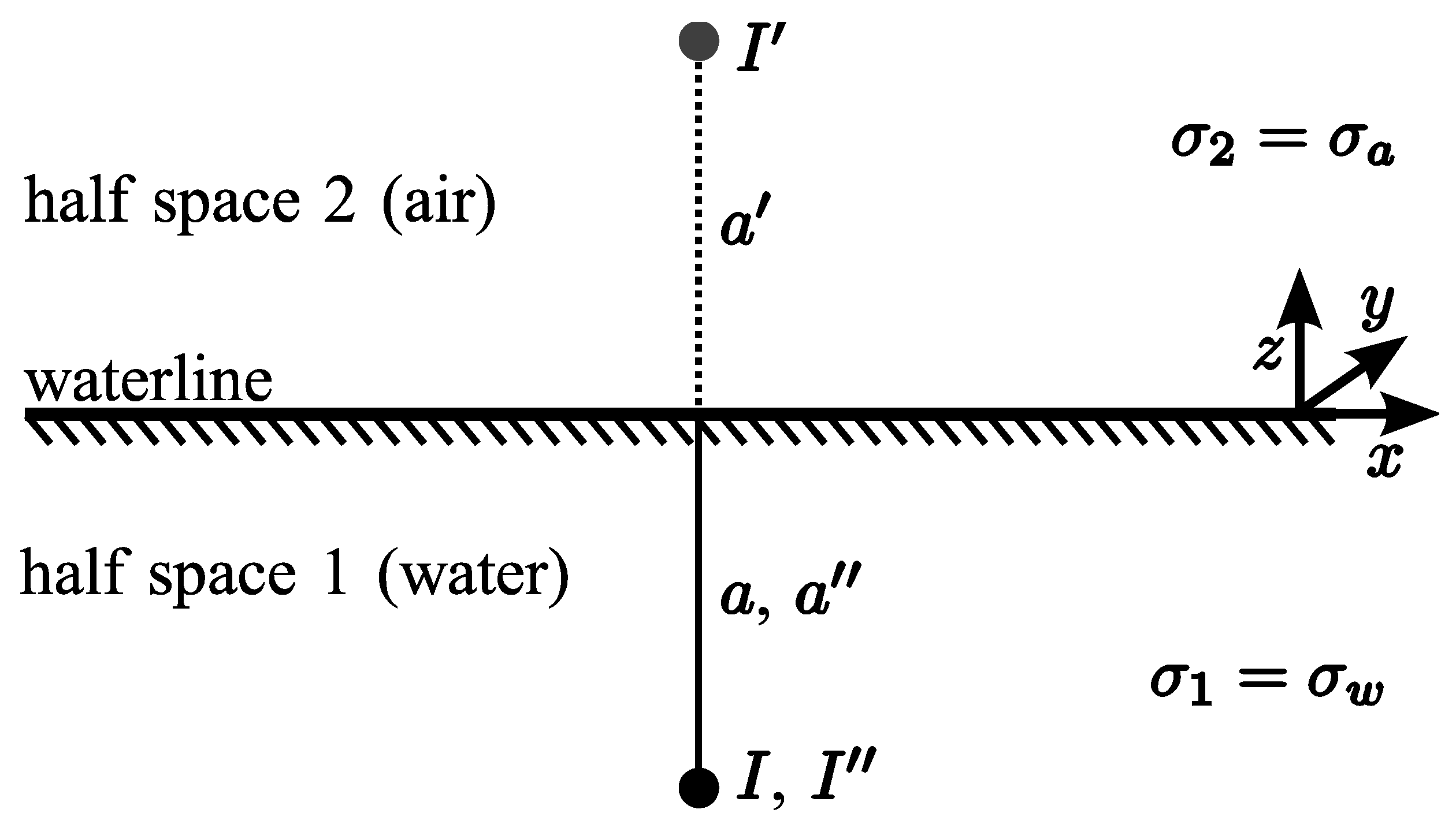
3.1. Method of Images for Conductive Media

In a homogeneous, conducting space with the boundary condition φ (∞) = 0, the electric potential of a current point source is described by:

$$\phi \left(\mathit{r}\right)=\frac{I}{4\pi \sigma \left|\mathit{r}-\mathit{\xi }\right|}.$$

(6)

Here, I is the impressed current, r is the position vector (receiving point), and ξ denotes the position of the point source. When a half space with another conductivity is brought into the vicinity of the current source, this can be considered by introducing several image sources, as depicted in Figure 2. Within the framework of the method of images, the potential distribution in the two half spaces is calculated separately in the sense of a case differentiation, where the point sources I and I′ are used for half space 1 (water), and point source I″ is considered for half space 2 (air). Please note that we first refer to a more general analysis of the current distribution within two conducting half spaces where we imply continuity for both the electric potential and the normal current density components at the boundary. Referring here to the specificities of the methods of images, the boundary value problem boils down to the following conditions:

$$a=a^{\prime }=a^{″}$$

(7)

$$I^{\prime }=\frac{{\sigma }_1- {\sigma }_2}{{\sigma }_1+{\sigma }_2}\cdot I$$

(8)

$$I^{″}=\frac{2{\sigma }_2}{{\sigma }_1+{\sigma }_2}\cdot I$$

(9)

Here, the conductivity of the water is σ₁, whereas in the subsequent step where the realistic water–air interface is then taken into account the conductivity of the air ${\sigma }_2$ is set to zero:

$${\sigma }_1={\sigma }_{\mathrm{w}}$$

(10)

$${\sigma }_2={\sigma }_{\mathrm{a}}=0$$

(11)

This leads to:

$$I^{\prime }=\frac{{\sigma }_{\mathrm{w}}-{\sigma }_{\mathrm{a}}}{{\sigma }_{\mathrm{w}}+{\sigma }_{\mathrm{a}}}\cdot I$$

(12)

$$=I$$

(13)

$$I^{″}=\frac{2{\sigma }_{\mathrm{a}}}{{\sigma }_{\mathrm{w}}+{\sigma }_{\mathrm{a}}}\cdot I$$

(14)

$$=0$$

(15)

The potential distribution below the waterline can now be derived using the superposition principle:

$${\phi }_{\mathrm{w}}\left(\mathit{r}\right)=\frac{I}{4\pi {\sigma }_{\mathrm{w}}}\cdot \left(\frac{1}{\left|\mathit{r}-\mathit{\xi }\right|}+\frac{1}{\left|\mathit{r}-{\mathit{\xi }}^{\prime }\right|}\right).$$

(16)

Here, ξ′ is the position vector of the image source I′. To calculate the potential in air, the current I in Equation (6) has to be substituted by (14) instead of (15), so that the fraction can be reduced by ${\sigma }_{\mathrm{a}}$:

$${\phi }_{\mathrm{a}}\left(\mathit{r}\right)=\frac{I^{″}}{4\pi {\sigma }_{\mathrm{a}}\left|\mathit{r}-\mathit{\xi }\right|},$$

(17)

$$=\frac{2{\sigma }_{\mathrm{a}}}{{\sigma }_{\mathrm{w}}+{\sigma }_{\mathrm{a}}}\cdot \frac{I}{4\pi {\sigma }_{\mathrm{a}}\left|\mathit{r}-\mathit{\xi }\right|},$$

(18)

$$=\frac{2I}{4\pi {\sigma }_{\mathrm{w}}\left|\mathit{r}-\mathit{\xi }\right|}.$$

(19)

Equation (19) contains an interesting result: the AEP distribution is exactly the same, as if the complete space would be filled with water and the impressed currents were doubled. This statement is also valid for the electric field [5,6].

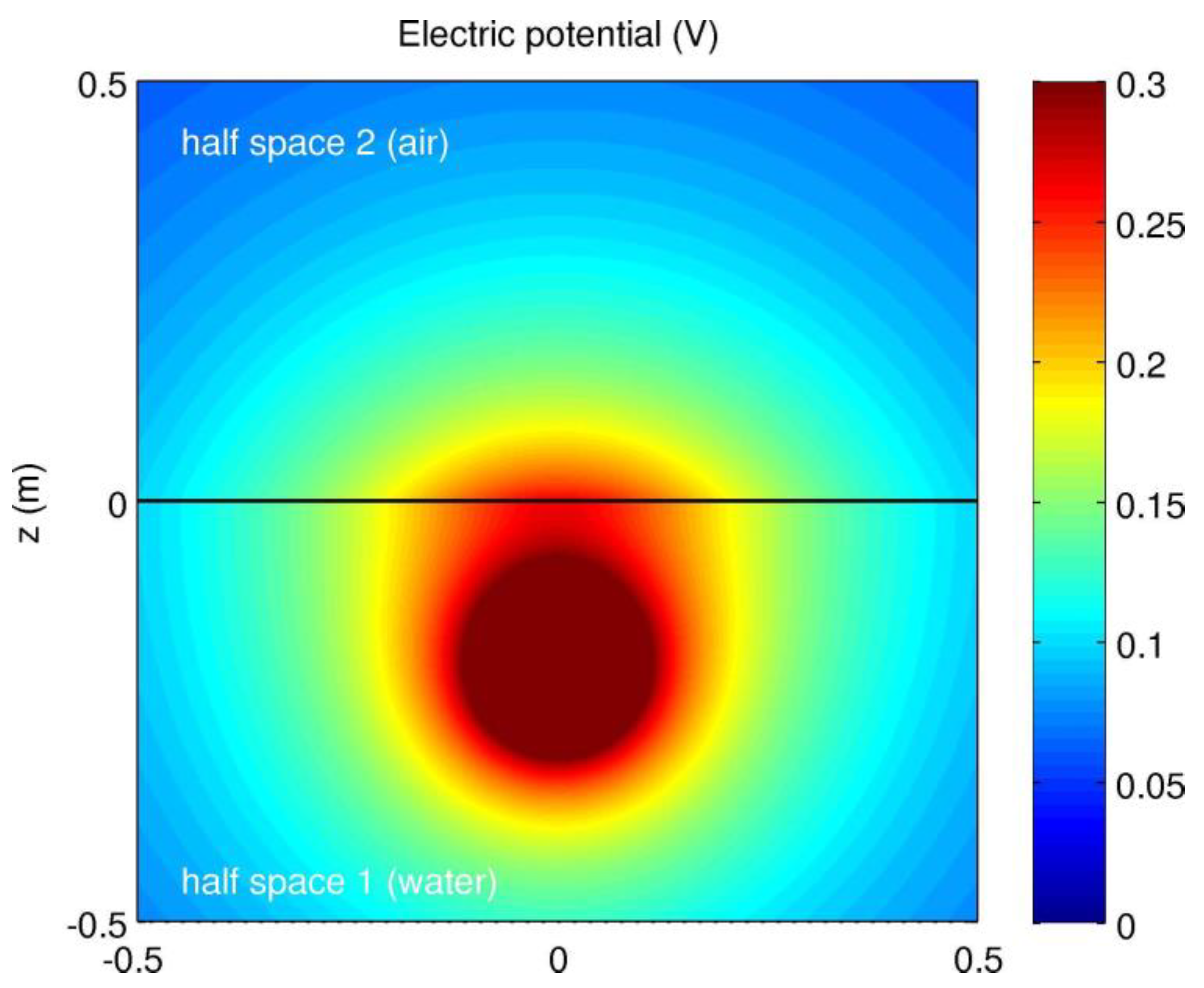
3.2. Analytical Calculation of a Point Current Source

To create a visual understanding of the derived field distributions, Equations (16) and (19) are evaluated and plotted in Figure 3 as an example. The example consists of a single current source with I = 1 A at the position ξ = (0, 0, −20 cm)^T below the waterline.

4. Numerical Simulation Approach

The numerical simulation of AEP signatures is based on the same idea and conditions as the analytical calculation: the continuity of the electric potential at the waterline. Since the method of images is not generally applicable, a kind of multiphysical approach is followed instead, where the simulation of the stationary current density distribution (underwater) is coupled to the calculation of electrostatic fields (above water).

4.1. Finite Element Method (FEM) Simulation Using COMSOL Multiphysics

The finite element method (FEM) tool COMSOL Multiphysics with the AC/DC module [7] was used to accomplish the numerical simulations of the three-dimensional (3D) electric field/stationary current analysis. As a first step, the stationary current density distribution was simulated using the Electric currents physics mode, and defining the waterline as a Neumann boundary condition:

$$\frac{\partial \phi }{\partial n}=0.$$

(20)

The electric potential at the waterline was then extracted and utilized to excite a second simulation with the Electrostatics physics mode. To realize a distant boundary condition, so-called infinite elements were attached to the outside boundary of the whole simulation domain, visible as additional layers on the water-/air-box (Figure 4; Figures 6–10). Additionally, the relative error is calculated and shown in Figure 5.

The simulation approach described above is not limited to the use of COMSOL, but it can be applied for any other FEM, boundary element method (BEM) or finite difference method (FDM) simulation software which provides multiphysics capabilities.

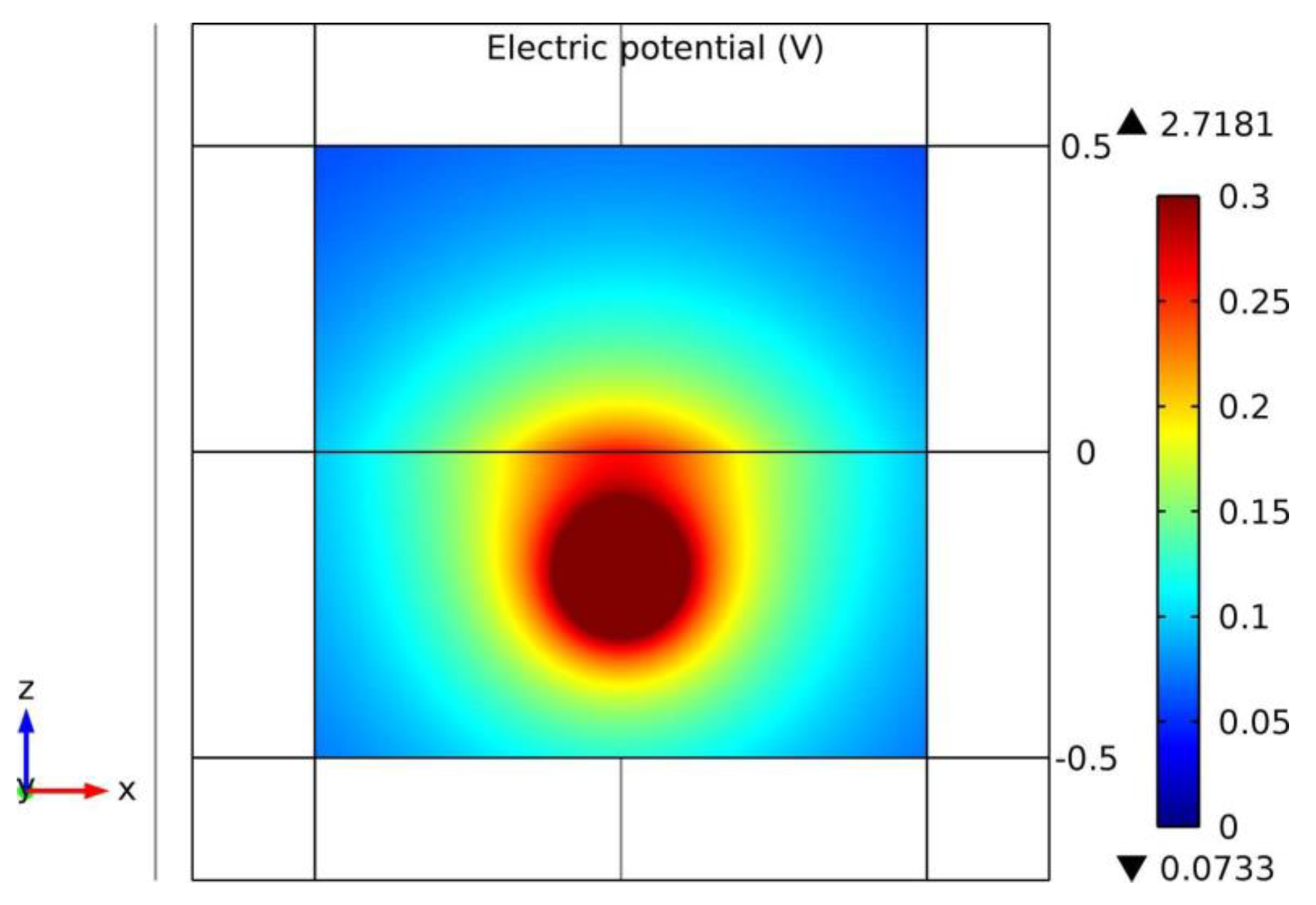
4.2. Numerical Simulation of a Point Current Source

To compare the analytical and numerical approaches, the same current point source (I = 1 A at the position ξ = (0, 0, −20 cm)^T that was previously calculated in Section 3.2, was simulated with COMSOL Multiphysics (5.4, COMSOL Multiphysics GmbH, Göttingen, Germany). As expected, the visualization of the relative error in Figure 5 shows that the numerical results were in good agreement with the analytical results. The higher error values of about 4% at the outer boundaries resulted from the imperfection of the infinite elements and could be further reduced by increasing their size or by refining their discretization.

The absolute value of the electric field is displayed in Figure 6. Assuming the same distance from the source, the AEP fields were twice as strong as the UEP fields, which could already be expected from Equation (19). Also notable is the zero-field point above the source, directly below the waterline, that occurs due to symmetry reasons.

Another interesting result is the surface charge distribution ${\zeta }_{\mathrm{wl}}$ on the waterline (Figure 7). It can be understood as the actual excitation source for the above-water electrostatic fields, and is calculated directly from the electric flux density:

$${\zeta }_{\mathrm{wl}}={\mathit{n}}_{12}\cdot \left({\mathit{D}}_2-{\mathit{D}}_1\right)$$

(21)

$$=D_{\mathrm{z}2}-D_{\mathrm{z}1}$$

(22)

$$=D_{\mathrm{z}2}$$

(23)

Note that at the waterline D_z1 is zero due to the Neumann boundary condition.

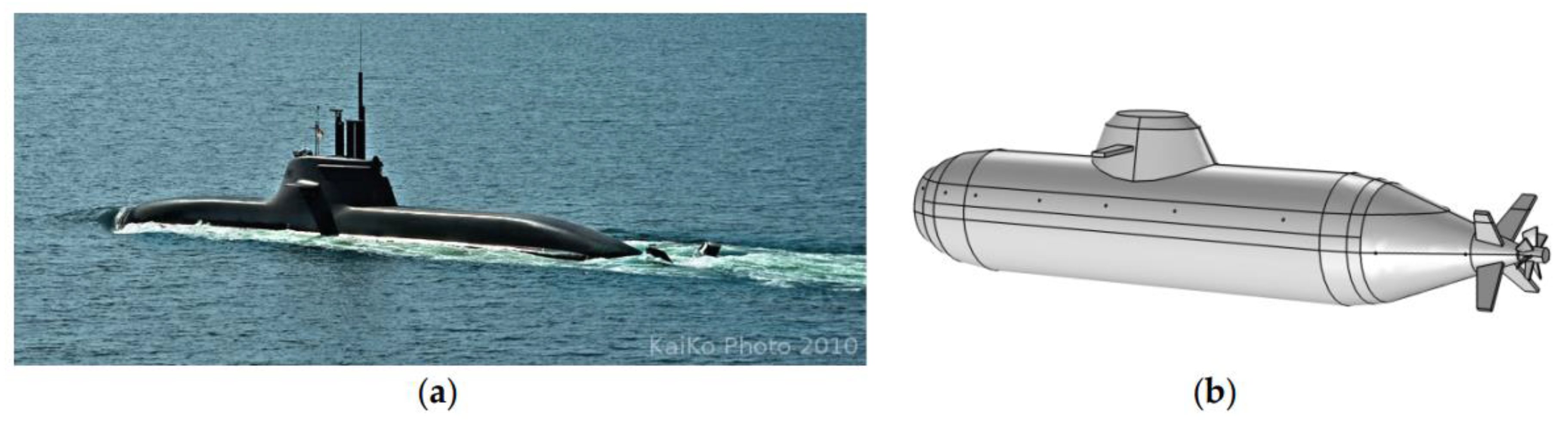
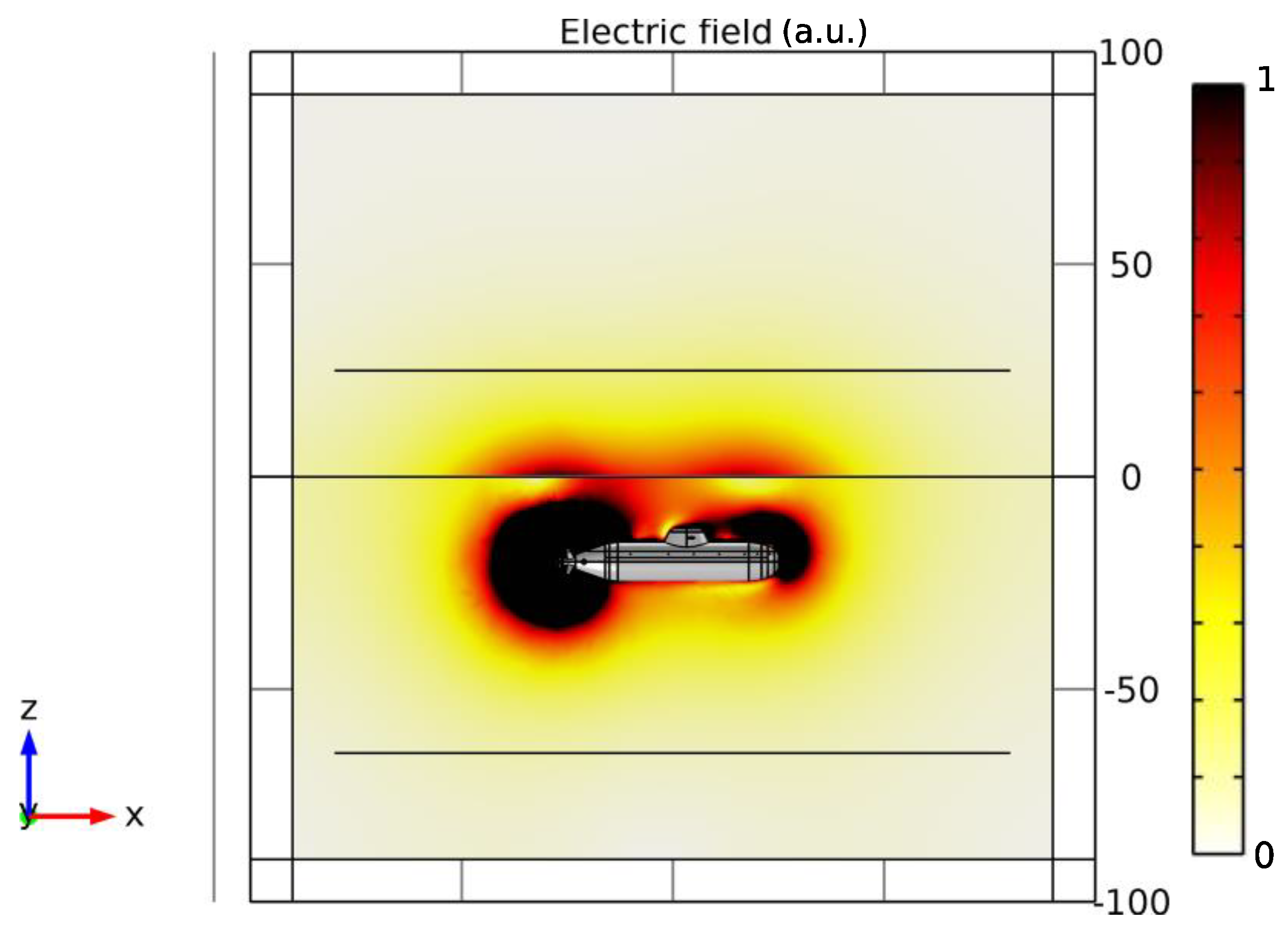
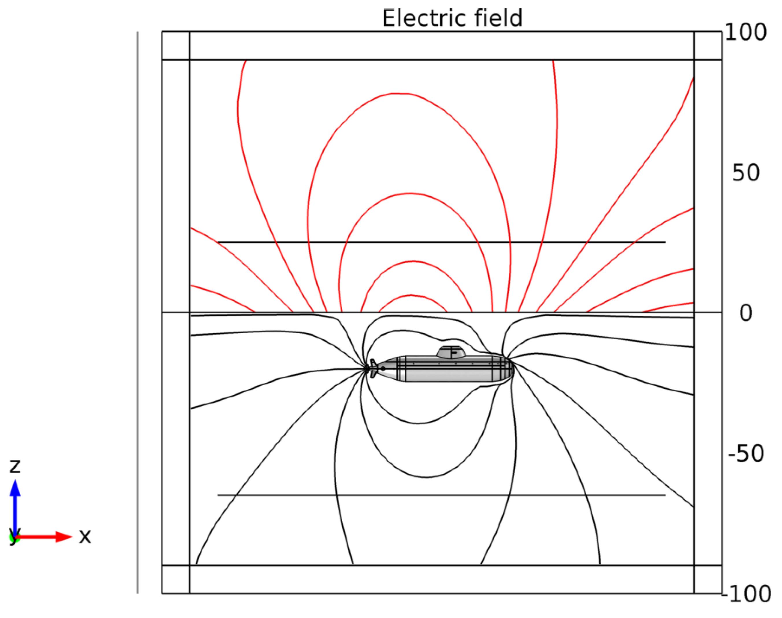
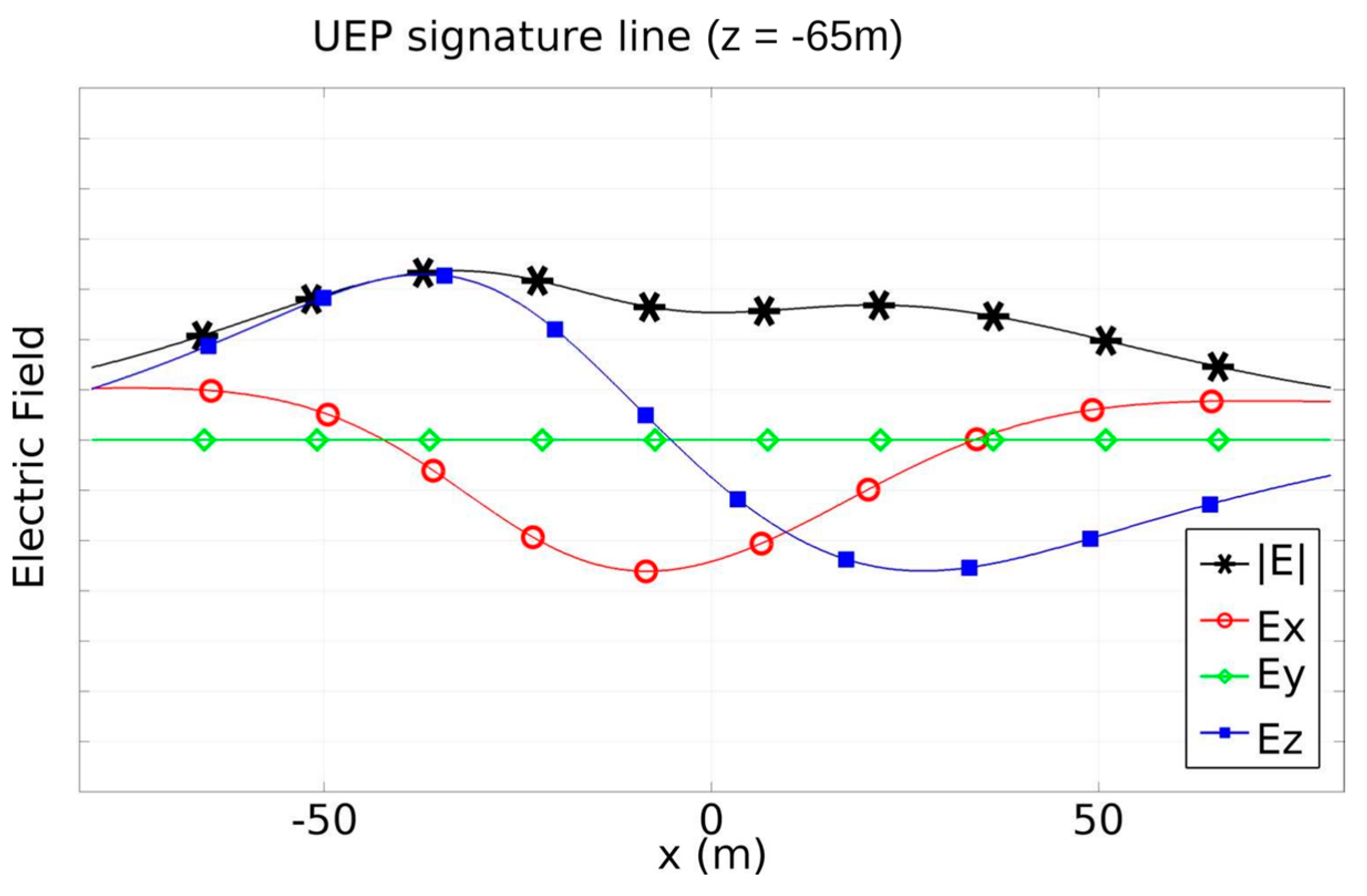
5. Numerical Simulation of a Submarine Model

After the simulation approach was verified for the point source excitation, it could then be applied to more complex and realistic scenarios (e.g., the signature simulation of naval vessels). Figure 8, Figure 9, Figure 10, Figure 11 and Figure 12 visualize the simulation results for a 50-m-long submarine model with sacrificial anode corrosion protection (SACP) that was submerged to a depth of z_s = −20 m below the waterline. Non-linear polarization curves of the material were considered to model the electrochemical behavior at the metal–water interfaces [5,8]. The electric potential distribution for the submarine model is displayed in Figure 8, indicating a dipole characteristic of the far field of the submarine. The two black lines above and below the waterline (Figure 8, Figure 9 and Figure 10) represent the evaluation location of the UEP signature line (Figure 11) and the AEP signature line (Figure 12). The visualization of the electric field strength in Figure 9 again confirms that the AEP signature was stronger than the UEP signature for comparable distances from the source. Under water, the electric field lines (Figure 10) correspond to the flow direction of the electric currents, and can therefore never cross, start, or end at the waterline. Above water, the electric field is excited by the surface charge distribution at the metal–seawater interface (Figure 7), so the field lines are allowed to start or end at the waterline.

Figure 11 shows a UEP signature line, which is the most commonly used representation for UEP signatures and corresponds to a three-axis measurement of the electric field during a drive-by. The UEP signature line, as well as the corresponding AEP signature line in Figure 12, were evaluated at a distance of 40 m from the submarine model. By comparing the two signatures it can again be seen that the AEP field strength was about twice as strong as the UEP field strength.

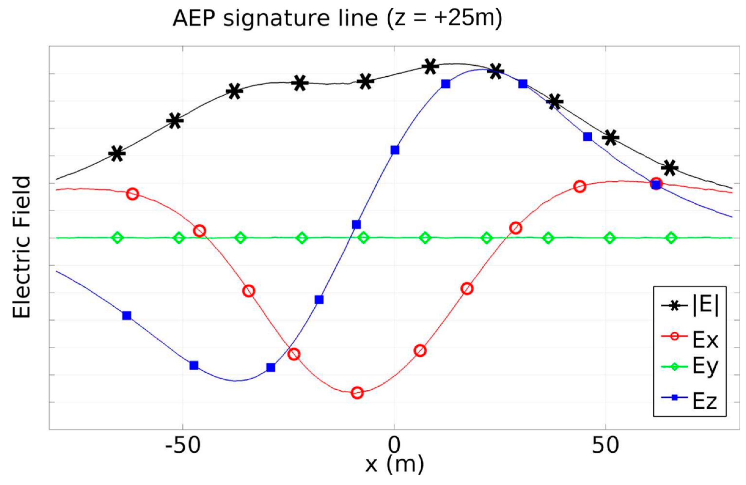
6. Relevance of AEP in the Context of ASW

In the area of magnetic signatures and ASW, the airborne detection of submarines, called magnetic anomaly detection (MAD), is already well established [9]. A typical MAD set-up contains a highly sensitive three-axis magnetometer, such as a SQUID (superconducting quantum interference device), that is mounted far underneath a helicopter. The important question is whether or not the corresponding exploitation scenario for electric signatures is realistic, or could at least become realistic in the future. The analytical investigations revealed that the AEP fields were approximately twice as strong as the UEP fields. However, this fact alone is not sufficient to appraise the relevance of AEP, because other parameters such as the signal-to-noise ratio (SNR) and the precision of electrostatic sensors have to be considered. In order to conduct a rough estimation, we start with the general rule that a common war ship produces UEP field strengths on the order of 1000 μV/m at a depth of 20 m below keel. As 20 m seems too small to be relevant for an AEP exploitation scenario, the electric field strength was translated to a distance of 40m. Assuming a dipole UEP field that has a decay ratio of 1/r³ for the electric field leads to:

$${\left|\mathit{E}\right|}_{\mathrm{UEP},\max }\left(\mathit{r}=40\mathrm{m}\right)=1000\frac{\mathsf{\mu }\mathrm{V}}{\mathrm{m}}\cdot \frac{{\left(20\mathrm{m}\right)}^3}{{\left(40\mathrm{m}\right)}^3}$$

(24)

$$=125\frac{\mathsf{\mu }\mathrm{V}}{\mathrm{m}},$$

(25)

$${\left|\mathit{E}\right|}_{\mathrm{AEP},\max }\left(\mathit{r}=40\mathrm{m}\right)=250\frac{\mathsf{\mu }\mathrm{V}}{\mathrm{m}}.$$

(26)

This value is far below the approximately 1 V/m precision state-of-the-art electric field mills sensors that are commonly used for airborne measurements of electrostatic fields in metrology. Additionally, the expected electric noise amplitude of over 100 V/m (Table 1) [10], similar to that caused by thunderstorms, or compared to one of the lowest electric fields on Earth found in the lower stratosphere on the order of 1 V/m [11], the order of magnitude is significantly higher than the expected AEP fields, which leads to a very low SNR. Therefore, a successful exploitation of AEP signatures via airborne sensors seems unrealistic, even if sensor technology improves sufficiently.

7. Conclusions

The technological progress of naval weapon systems and corresponding countermeasures continuously opens new areas of interest. In this context, we investigated the so far neglected AEP signature, which is directly connected to the UEP signature. First, we presented an analytical calculation approach for AEP signatures based on the method of images that can be used for simple geometries. Here, we observed that the AEP fields were twice as strong as UEP fields at the same distance to the excitation. Following this, we explained in detail how to numerically simulate AEP signatures by coupling the simulation of the stationary current density distribution with an electrostatic simulation. By evaluating an example scenario with a single current point source below the waterline, we were able to show that the analytically and numerically calculated AEP fields were in agreement. The multiphysical approach was then applied to the simulation of a realistic submarine model, considering non-linear polarization curves to reproduce the electrochemical behavior at the metal–seawater interfaces. Both numerical simulations confirmed the analytically established doubling of the AEP fields. Finally, we discussed the relevance of AEP in the context of anti-submarine warfare (ASW). A rough estimation of expectable AEP field strength in respect to electric noise indicated that the SNR is generally too low for a successful exploitation of AEP signatures via airborne assessment.

References

1. Holmes, J. Exploitation of a Ship’s Magnetic Field Signatures, 1st ed.; Morgan & Claypool: Williston, VT, USA, 2006. [Google Scholar]
2. Jackson, J. Classical Electrodynamics, 3rd ed.; John Wiley & Sons Inc.: Hoboken, NJ, USA, 1999. [Google Scholar]
3. Schaefer, D.; Doose, J.; Rennings, A.; Erni, D. Above water electric potential signatures and their relevance in the context of ASW. In Proceedings of the MARELEC Conference, Hamburg, Germany, 16–18 July 2013. [Google Scholar]
4. Schaefer, D.; Doose, J.; Pichlmaier, M.; Rennings, A.; Erni, D. Conversion of UEP signatures between different environmental conditions using shaft currents. IEEE J. Oceanic Eng. 2016, 41, 105–111. [Google Scholar] [CrossRef]
5. Schaefer, D. Vorhersage und Umrechnung korrosionsbedingter UEP-Signaturen von Wasserfahrzeugen. Ph.D. Thesis, University of Duisburg-Essen, Duisburg, Germany, 2015. [Google Scholar]
6. Scheible, J. Die Lösung des feldtheoretischen Viermedienproblems ebener Schichten. Archiv für Elektrotechnik 1991, 75, 9–17. [Google Scholar] [CrossRef]
7. COMSOL Group, “COMSOL Multiphysics (FEM)—AC/DC Module”. Available online: https://www.comsol.com/acdc-module (accessed on 11 December 2019).
8. Schaefer, D.; Zion, S.; Doose, J.; Rennings, A.; Erni, D. Numerical simulation of UEP signatures with propeller-induced ULF modulations in maritime ICCP systems. In Proceedings of the MARELEC Conference, San Diego, CA, USA, 20–23 June 2011. [Google Scholar]
9. Hirota, M.; Furuse, T.; Ebana, K.; Kubo, H.; Tsushima, K.; Inaba, T.; Shima, A.; Fujinuma, M.; Tojyo, N. Magnetic detection of a surface ship by an airborne LTS SQUID MAD. IEEE Trans. Appl. Supercond. 2001, 2, 884–887. [Google Scholar] [CrossRef]
10. Hoppel, W.A.; Gathman, S.G. Experimental determination of the eddy diffusion coefficient over the open ocean from atmospheric electric measurements. J. Phys. Oceanogr. 1972, 2, 248–254. [Google Scholar] [CrossRef]
11. Nicoll, K.A. Measurements of atmospheric electricity aloft. Surv. Geophys. 2012, 33, 991–1057. [Google Scholar] [CrossRef]
Figure 1. (a) Photo of a type 212A submarine and (b) the geometry of the numerical submarine model for simulating the AEP signature.
Jmse 07 00053 g001
Figure 2. Setup for the method of images. The vicinity of a conducting half-space in front of a point current source I can be considered by introducing the image sources I′ and I″.
Jmse 07 00053 g002
Figure 3. Analytically calculated electric potential distribution for a single current source I with considered values of I = 1 A and ξ = (0, 0, −20 cm)T.
Jmse 07 00053 g003
Figure 4. Numerically simulated electric potential distribution, for a single current source I with considered values I = 1 A and ξ = (0, 0, −20 cm)T.
Jmse 07 00053 g004
Figure 5. Relative error calculated as the absolute value of the difference between the electric potential (Figure 3 and Figure 4) divided by their mean value.
Jmse 07 00053 g005
Figure 6. Numerically simulated absolute value of the electric field for a single current source I with considered values I = 1 A and ξ = (0, 0, −20 cm)T.
Jmse 07 00053 g006
Figure 7. Numerically simulated absolute value of the surface charge density ζ wl at the water–air interface, for a single current source I with considered values I = 1 A and ξ = (0, 0, −20 cm)T.
Jmse 07 00053 g007
Figure 8. Numerically simulated potential distribution for a submarine model. The two black lines represent the evaluation location of the underwater electric potential (UEP) signature (zu = −65 m, Figure 11) and the above-water electric potential (AEP) signature (za = +25 m, Figure 12).
Jmse 07 00053 g008
Figure 9. Numerically simulated absolute value of the electric field for a submarine model.
Jmse 07 00053 g009
Figure 10. Numerically simulated electric field lines for a submarine model. The distance between the field lines does not represent the electric field strength, because the seeding points for the field lines were set manually.
Jmse 07 00053 g010
Figure 11. Numerically simulated UEP signature line for a submarine model. The fields were sampled along the sensor line in the x-direction at a constant height of zu = −65 m below the waterline (40 m below the keel of the submarine). The ordinate scale is the same as in Figure 12.
Jmse 07 00053 g011
Figure 12. Numerically simulated AEP signature line for a submarine model. The fields were sampled along the sensor line in the x-direction at a constant height of zu = +25 m below the waterline (40 m above the keel of the submarine). The ordinate scale is the same as in Figure 11.
Jmse 07 00053 g012