Sliding Mode Control in Backstepping Framework for a Class of Nonlinear Systems

Abstract

Both backstepping control (BC) and sliding mode control (SMC) have been studied extensively over the past few decades, and many variations of controller designs based on them can be found in the literature. In this paper, sliding mode control in a backstepping framework (SBC) for a class of nonlinear systems is proposed and its connections to SMC studied. SMC is shown to be a special case of SBC. Without losing generality, the regulation control problem is studied, while tracking control is achieved by replacing the states with the difference between the states and their desired values. The SBCs are designed for nonlinear single-input-single-output (SISO) and multiple-input-multiple-output (MIMO) systems with the presence of bounded uncertainties from unmodeled dynamics, parametric variations, disturbances, and measurement noise, and the closed loop systems are proven to be asymptotically stable using the Lyapunov stability theory. The comparison of SBC to SMC from the design process, chattering effects, and chatter reduction are also discussed. SBC inherits the merits of backstepping control in choosing gains independently, while leveraging useful nonlinear dynamics for controller design simplification. Hence, it provides more flexibility in controller design in the sense of controlling coverage speed and making use of useful nonlinearities in the dynamics. To demonstrate the effectiveness of SBC, an application on cruise tracking control of an autonomous underwater vehicle was studied.

1. Introduction

The backstepping method breaks the problem of controlling complex higher order systems into a sequence of lower order control problems through a recursive procedure. By doing this, the flexibility in these lower order systems can be explored for controller design, which makes the control less restrictive in system complexity requirements, compared to other methods [1]. Over the past few decades, backstepping control has been studied extensively with applications for the control of spacecraft and aircraft [2,3,4,5], marine vessels [6,7,8], various motors [9,10,11], robotic manipulators and systems [12,13,14], and many others [15,16,17,18].

Numerous variations of backstepping control can be found in the literature. Specific formulations exist for nonlinear systems with time delays [19], systems with structural obstacles in obtaining continuous feedback laws [20], time-varying systems [21], nonlinear systems with block structures [22], plants with unknown backlash nonlinearities [23], nonholonomic systems with strong nonlinear drifts [24], systems with unknown dead-zone non-linearity [25], nonlinear systems with delay of neutral type [26], and so on. The backstepping method is also used to assist in design for fuzzy control [27,28,29], neural network control [25,30,31,32,33,34], and wavelet adaptive control [35,36]. Another related topic is robust backstepping control (RBC), which focuses on handling uncertainties from un-modeled dynamics (i.e., imperfection or simplification in modeling and variations in system parameters), noise in measurements, and disturbances [37,38,39].

Aside from RBC, sliding mode control (SMC) is another Lyapunov-based robust control method, which has attracted much attention from both the industry and academia [40]. SMC produces a switching control law to force the system to converge to the sliding surface while trapping the system within a boundary layer near the sliding surface under the guidance of the Lyapunov stability theory [41,42]. Due to the nature of switching control law, the chattering problem associated with the controller has also caught the attention of researchers. Many solutions can be found in [43,44,45,46]. There is also some research that combines backstepping and sliding mode methods to design controllers for special applications such as the adaptive backstepping sliding mode control for linear induction motor drives presented in [47].

In this paper, a systematic SBC design is formulated for both single-input-single-output (SISO) systems and multiple-input-multiple-output (MIMO) systems. The general nonlinear system considered here is in a recursive form. Systems not in the standard form can be converted to the standard form using input-output linearization or other methods. Starting from the recursive model, an SBC is designed to guarantee that the closed loop system is asymptotically stable. The proposed controller is also compared to the popular SMC on simplicity of design, uncertainty handling, and chatter reduction. Further, the design of integral SBC (ISBC) is presented. It is found that SBC and ISBC retain the advantages of both the robustness of SMC and the simplicity of backstepping control. The proposed SBC/ISBC methods provide more flexibility in controlling the convergence speed of the closed loop system, while retaining the ability to leverage useful nonlinear dynamics toward a simpler control law. The main contributions of this paper are as follows: (1) SBC and ISBC for a class of nonlinear systems are proposed; (2) the controller design formulations reveal both the equivalence and difference between SBC/ISBC and SMC/ISMC; and (3) it demonstrates that the proposed SBC/ISBC are more flexible design and can achieve better performance than the traditional SMC/ISMC.

The rest of the paper is organized as follows: in Section 2, the SBC for nonlinear SISO system is presented. The results for MIMO system are given in Section 3. In Section 4, the SBC is compared to SMC in terms of simplicity of design, chatter effects, and some additional performance metrics. Section 5 details a benchmark control example using the proposed SBC method to illustrative the effectiveness of the controller. Finally, conclusions are drawn in Section 6.

2. SBC of SISO Systems

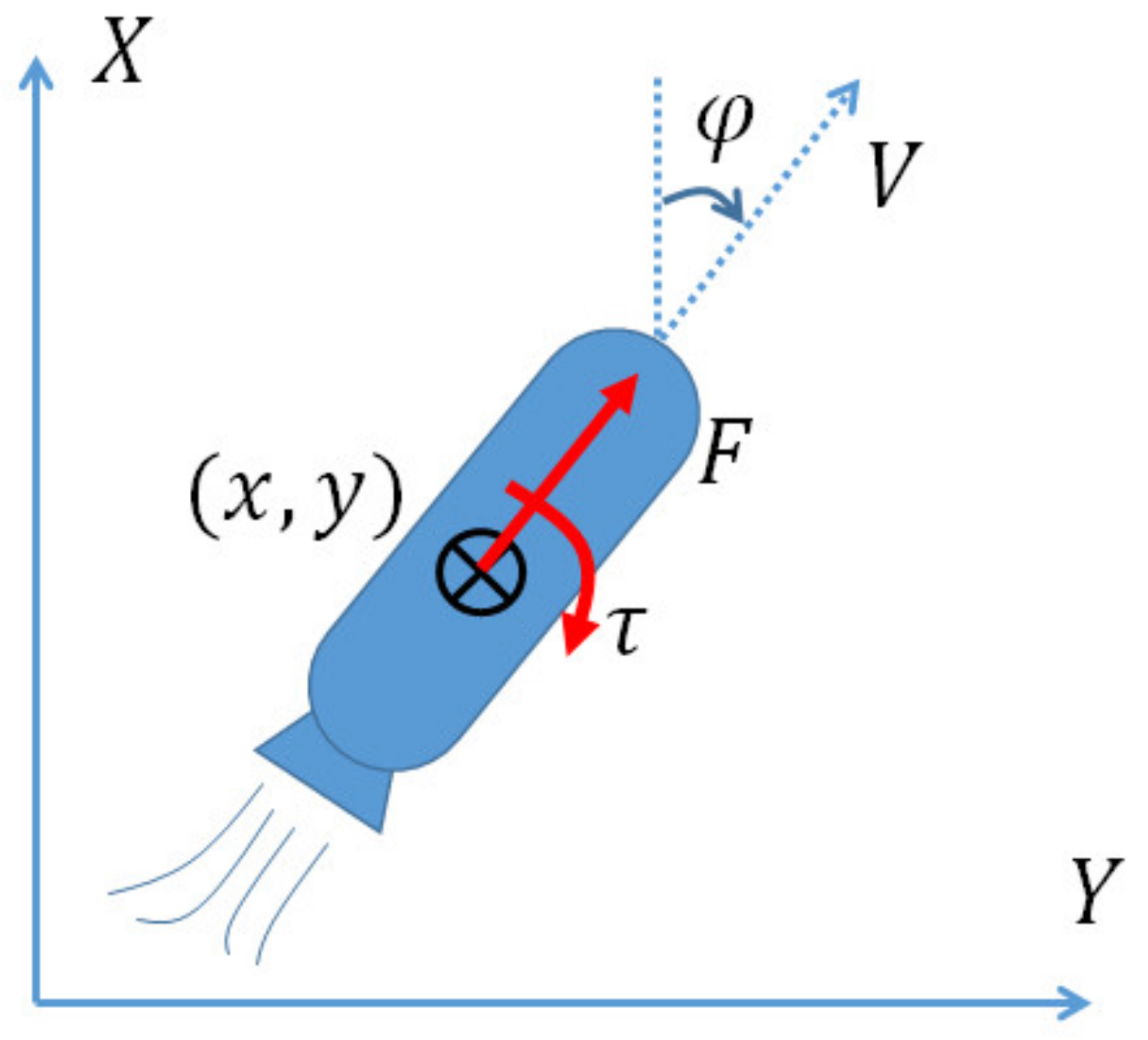
2.1. Problem Formulation

The nonlinear SISO system considered in this paper is assumed to have the following form (or, the system is assumed to be input-output linearizable to have the following form):

$$x^{\left(n\right)}=f\left(x\right)+g(x)u$$

(1)

where $x$ is the state variable, composed of the state and its derivatives up to the order of $n$, and both $f\left(x\right)$ and $g(x)$ are nonlinear functions of $x$. Without special notices, all scalar functions are in regular style, while vectors and matrices will be in bold.

Remark 1.

For a general nonlinear system given in a more general form as:

$$\left\{\begin{array}{c}{\dot{x}}_1=f_1\left(x\right)\hfill \\ {\dot{x}}_2=f_2\left(x\right)\hfill \\ \begin{array}{cc}\hfill & ⋮\hfill \end{array}\hfill \\ {\dot{x}}_n=f_n\left(x\right)+g_1\left(x\right)u\hfill \end{array}\right.$$

(2)

and assuming the output function is given as $y=h\left(x\right)$, then, the system can be linearized using input-output linearization, which results in

$$\left\{\begin{array}{c}\dot{y}={\ell }_{f}h\left(x\right)+{\ell }_{g}h\left(x\right)u\hfill \\ \ddot{y}={\ell }_{f^{\left(2\right)}}h\left(x\right)+{\ell }_g{\ell }_{f}h\left(x\right)u\hfill \\ \begin{array}{cc}\hfill & ⋮\hfill \end{array}\hfill \\ y^{\left(r\right)}={\ell }_{f^{\left(r\right)}}h\left(x\right)+{\ell }_g{\ell }_{f^{\left(r-1\right)}}h\left(x\right)u\hfill \end{array}\right.$$

(3)

where $\ell$ represents the Lie derivative operator and $r$ is the relative degree of the system. We know that:

$${\ell }_{g}h\left(x\right)={\ell }_g{\ell }_{f}h\left(x\right)=\cdots {\ell }_g{\ell }_{f^{\left(r-2\right)}}h\left(x\right)=0$$

(4)

and

$${\ell }_g{\ell }_{f^{\left(r-1\right)}}h\left(x\right)\ne 0$$

(5)

By defining the new states ${\xi }_1=y$, ${\xi }_2=\dot{y}$,$\cdots , {\xi }_r=y^{\left(r-1\right)}$, the general nonlinear system in (2) can be written in the form of (1).

Remark 2.

Without losing generality, the regulation problem (i.e., $\underset{t\to \infty }{\lim }x=0$ for SISO system or $\underset{t\to \infty }{\lim }x=0\in {\mathbb{R}}^m$ for MIMO systems) will be considered in this paper. For tracking problems where $\underset{t\to \infty }{\lim }x=x_d$ or $\underset{t\to \infty }{\lim }x=x_d\in {\mathbb{R}}^m$, new state variables $\tilde{x}=x-x_d$ or $\tilde{x}=x-x_d$ can be defined to convert the tracking problem to a regulation problem.

Since the standard backstepping method breaks a complex system into a lower order system to simplify the controller design process, system (1) is firstly written into the following canonical form as:

$$\left\{\begin{array}{c}{\dot{x}}_1=x_2\hfill \\ {\dot{x}}_2=x_3\hfill \\ \begin{array}{cc}\hfill & ⋮\hfill \end{array}\hfill \\ {\dot{x}}_n=f\left(x\right)+g(x)u\hfill \end{array}\right.$$

(6)

Following the standard Backstepping control design, the first new state $z_1$ is defined as $z_1=x_1$. Then, we take the derivative of $z_1$ to get ${\dot{z}}_1=-{\gamma }_1{z}_1+\underset{z_2}{\underbrace{\left({\gamma }_1{z}_1+{\dot{x}}_1\right)}}$. Hence, $z_2$ can be defined as $z_2={\gamma }_1{z}_1+{\dot{x}}_1={\gamma }_1{x}_1+x_2$. We repeat this process until $z_{n-1}$. Since the system in (6) is already in canonical form, this process can be described using the following transformation:

$$z_i=\left({{\displaystyle \prod }}_{j=1}^{i-1}\left(\frac{d}{\mathrm{dt}}+{\gamma }_j\right)\right)x, 1<i\le n$$

(7)

It is easy to verify that under the transformation given in (7), the system in Equation (6) can be converted into the following recursive structure:

$$\left\{\begin{array}{c}{\dot{z}}_1=-{\gamma }_1{z}_1+z_2\hfill \\ {\dot{z}}_2=-{\gamma }_2{z}_2+z_3\hfill \\ \begin{array}{cc}\hfill & ⋮\hfill \end{array}\hfill \\ {\dot{z}}_n=v\hfill \end{array}\right.$$

(8)

where ${\gamma }_i>0, i=1,2,\cdots ,n$ are positive real numbers. For simplicity, we can write $v={\dot{z}}_n=\frac{d}{\mathrm{dt}}\left(x_n+{{\displaystyle \sum }}_{j=1}^{n-1}{\alpha }_j{x}_j\right)={\dot{x}}_n+{{\displaystyle \sum }}_{j=1}^{n-1}{\alpha }_j{x}_{j+1}$, and ${\alpha }_j$ are functions of an independent scalar set $\left\{{\gamma }_n,{\gamma }_{n-1},\cdots ,{\gamma }_1\right\}$, i.e., ${\alpha }_1={\gamma }_1{\gamma }_2\cdots {\gamma }_n$ and ${\alpha }_{n-1}={{\displaystyle \sum }}_{j=1}^n{\gamma }_j$.

Without consideration for robustness, the traditional backstepping controller can be derived, such that $v=-{\gamma }_n{z}_n$, which results in a controller of the form:

$$u=\frac{1}{g\left(x\right)}\left(-f\left(x\right)-d\left(x\right)-{\gamma }_n{z}_n\right)$$

(9)

where $d\left(x\right)={{\displaystyle \sum }}_{j=1}^{n-1}{\alpha }_j{x}_{j+1}$. This makes the system “theoretically” exponentially stable. Here, “theoretically” means that this is only guaranteed to be true when all sources of uncertainties do not exist. Alternatively, the controller that ensures $v=-{\gamma }_{n}sgn(z_n)$ is given by:

$$u=\frac{1}{g\left(x\right)}\left(-f\left(x\right)-d\left(x\right)-{\gamma }_{n}sgn(z_n)\right)$$

(10)

Since ${\gamma }_n$ is a user-defined constant parameter, the control formulations in (9) and (10) are not robust.

2.2. SBC Design

Before moving on to the SBC design, the following assumption is made to quantify the uncertainties from un-modeled dynamics, parameter variation, noise, and disturbances.

Assumption 1.

The matching conditions requirement assumes that in (1) the uncertainty of $f$ and $g$ satisfy the following:

$$\left\{\begin{array}{c}\left|f-\widehat{f}\right| \le F_f\hfill \\ \left|d-\widehat{d}\right| \le F_d, d={\displaystyle \sum }_{j=1}^{n-1}{\alpha }_j{x}_{j+1}\hfill \\ \widehat{g}=\left(1+\Delta \right)g, \left|\Delta \right|\le G<1\hfill \end{array}\right.$$

(11)

where $F_f$ and $F_d$ are the upper bound of the uncertainties of $f\left(x\right)$ and $d\left(x\right)$, and $\Delta$ is the difference between $g\left(x\right)$ and $\widehat{g}\left(x\right)$, and $G$ is the upper bound of $\left|\Delta \right|$.

Theorem 1.

For a class of nonlinear system given in form of (1) or the equivalent canonical form of (8), which meets the uncertainty bounds or matching condition of (11), a nonlinear SBC control is given by:

$$u=\frac{1}{\widehat{g}\left(x\right)}\left[-\widehat{f}\left(x\right)-\widehat{d}\left(x\right)-ksgn(s\right)]$$

(12)

where

$$s=z_n=\left({{\displaystyle \prod }}_{j=1}^{n-1}\left(\frac{d}{\mathrm{dt}}+{\gamma }_j\right)\right)x=x_n+{{\displaystyle \sum }}_{j=1}^{n-1}{\alpha }_j{x}_j,$$

(13)

and the control gain is chosen as

$$k\ge \frac{1}{1-G}\left(F_f+F_d+G\left|\widehat{f}\left(x\right)+\widehat{d}\left(x\right)\right|+\eta \right)$$

(14)

where $\eta$ is an arbitrary positive scalar, and the sign function is given by

$$sgn(s)=\left\{\begin{array}{c}-1 if s<0\hfill \\ 0 if s=0\hfill \\ 1 if s>0\hfill \end{array}\right.$$

(15)

Then, the system is asymptotically stable.

Remark 3.

Since $G<1$, the positive control gain in (14) always exists and can further be chosen as equality for simplicity, which gives:

$$k=\frac{1}{1-G}\left(F_f+F_d+G\left|\widehat{f}\left(x\right)+\widehat{d}\left(x\right)\right|+\eta \right)$$

(16)

Proof. 

To prove Theorem 1, we choose the positive definite Lyapunov function $V=\frac{1}{2}{s}^2$. Its derivative becomes:

$$\begin{array}{cc}\hfill \dot{V}& =s\dot{s}=s\left({\dot{z}}_n\right)=s\left(d\left(x\right)+{\dot{x}}_n\right)\hfill \\ & =s\left(d\left(x\right)+f\left(x\right)+g(x)u\right)\hfill \\ & =s\left(\begin{array}{c}d\left(x\right)+f\left(x\right)+g(x)\frac{1}{\widehat{g}\left(x\right)}\cdot \hfill \\ \left[-\widehat{f}\left(x\right)-\widehat{d}\left(x\right)-ksgn(s\right)]\hfill \end{array}\right)\hfill \\ & =s\left(\begin{array}{c}d\left(x\right)+f\left(x\right)+\left(1+\Delta \right)\cdot \hfill \\ \left[-\widehat{f}\left(x\right)-\widehat{d}\left(x\right)-ksgn(s\right)]\hfill \end{array}\right)\hfill \\ & =s\left(\begin{array}{c}\left[f\left(x\right)-\widehat{f}\left(x\right)\left]+\right[d\left(x\right)-\widehat{d}\left(x\right)\right]\hfill \\ -\Delta \left[\widehat{f}\left(x\right)+\widehat{d}\left(x\right)\right]-\left(1+\Delta \right)ksgn(s)\hfill \end{array}\right)\hfill \\ & \le \left|s\right|\left(F_f+F_d+G\left|\widehat{f}\left(x\right)+\widehat{d}\left(x\right)\right|-\left(1-G\right)k\right)\hfill \end{array}$$

(17)

If $k$ is chosen large enough such that Equation (14) is satisfied, then, $\dot{V}\le -\eta \left|s\right|$, and thus the Lyapunov rate is strictly decreasing. According to the Lyapunov stability theorem, we can conclude that the system is asymptotically stable. □

2.3. Integral SBC Control

To eliminate the steady-state bias or shorten the rising time, an integral term is typically considered in the controller design. The importance of integral terms in backstepping control design has been demonstrated in [48]. Considering the system in (6), the integral sliding mode control in backstepping framework control (ISBC) can be implemented by adding another state $x_0={{\displaystyle \int }}_{t_0}^{t}x\left(\tau \right)d\tau$ to the system, which results in:

$$\left\{\begin{array}{c}{\dot{x}}_0=x_1\hfill \\ {\dot{x}}_1=x_2\hfill \\ \begin{array}{cc}\hfill & ⋮\hfill \end{array}\hfill \\ {\dot{x}}_n=f\left(x\right)+g(x)u\hfill \end{array}\right.$$

(18)

The results in Section 2 are valid for system (18), if we redefine the function $s\left(x\right)$ and $d\left(x\right)$ as follows:

$$s=z_n=\left({{\displaystyle \prod }}_{j=0}^{n-1}\left(\frac{d}{\mathrm{dt}}+{\gamma }_j\right)\right)x=x_n+{{\displaystyle \sum }}_{j=0}^{n-1}{\alpha }_j^{*}{x}_j$$

(19)

$$d={{\displaystyle \sum }}_{j=0}^{n-1}{\alpha }_j^{*}{x}_{j+1}$$

(20)

Then, the control law and the control gain update law are the same as those in Equations (13) and (14). For systems that need higher order integral control, the same method can be used to add new states.

2.4. Chattering Effects

As the sliding surface function used in the SBC design, denoted by $s$ in Equation (13), approaches zero, the sign function tends to switch at a high frequency. This chattering phenomenon and its reduction has been extensively studied for SMC, where there are two primary methods: the boundary layer method [42] and other surface approach dynamics (e.g., using saturation, arctangent function instead of sign function) [49], and higher order or nonlinear sliding surface functions [50,51]. Algorithms to eliminate chatter were also studied in [52] and the existence of a solution for nonlinear convergent chatter-free sliding mode control was studied in [53]. The same ideas can be used to reduce chatter in SBC design.

3. SBC of MIMO Systems

In this paper, a MIMO system of the following form is considered:

$$x_i^{\left(n_i\right)}=f_i\left(x\right)+{\displaystyle \sum }_{j=1}^m{g}_{i,j}\left(x\right) u_j \mathrm{and} i,j=1,2,\cdots ,m$$

(21)

where $x=\left[x_1,{\dot{x}}_1,\cdots ,x_1^{n_1},x_2,{\dot{x}}_2,\cdots ,x_2^{n_2},\cdots \right]$.

Remark 4.

The system discussed here refers to a fully-actuated system. The under- and over- actuated system control problems are solved with other techniques, which are beyond the scope of this paper and will not be discussed here.

Remark 5.

For a special class of MIMO Systems of the form ${\mathit{x}}^{\left(n\right)}=\mathit{f}\left(\mathit{x}\right)+\mathit{g}\left(\mathit{x}\right)\mathit{u}$, where $\mathit{x}$, $\mathit{f}$, $\mathit{u}\in {\mathbb{R}}^m$, $\mathit{g}\in {\mathbb{R}}^{m\times m}$. The controller in the same form can be obtained providing that $n_1=n_2=\cdots =n$.

To follow the derivation for SISO systems, the MIMO system in (21) is first written into the following canonical form:

$$\left\{\begin{array}{c}{\dot{x}}_{i,1}=x_{i,2}\hfill \\ {\dot{x}}_{i,2}=x_{i,3}\hfill \\ \begin{array}{cc}\hfill & ⋮\hfill \end{array}\hfill \\ {\dot{x}}_{i,n}=f_i\left(x\right)+{\displaystyle {\displaystyle \sum }_{j=1}^m}{g}_{i,j}\left(x\right) u_j\hfill \end{array}\right., i=1,2,\cdots m$$

(22)

Then, following the backstepping design for the SISO system, we get:

$$\left\{\begin{array}{c}{\dot{z}}_{i,1}=-{\gamma }_{i,1}{z}_{i,1}+z_{i,2}\hfill \\ {\dot{z}}_{i,2}=-{\gamma }_{i,2}{z}_{i,2}+z_{i,3}\hfill \\ \begin{array}{cc}\hfill & ⋮\hfill \end{array}\hfill \\ {\dot{z}}_{i,n_i}={{\displaystyle \sum }}_{j=1}^{n_i-1}{\alpha }_{i,j}{x}_{i,j+1}+{\dot{x}}_{i,n}\hfill \end{array}\right., i=1,2,\cdots m$$

(23)

Similarly, the matching conditions are given in assumption 2 as follows.

Assumption 2.

The matching conditions requirement assumes that the uncertainty of $\mathit{f}$ and $\mathit{g}$ in Equation (21) satisfy the following:

$$\left\{\begin{array}{c}\left|\mathit{f}-\widehat{\mathit{f}}\right|\le {\mathit{F}}_{\mathit{f}}\hfill \\ \left|\mathit{d}-\widehat{\mathit{d}}\right|\le {\mathit{F}}_{\mathit{d}}, d_i={{\displaystyle \sum }}_{j=1}^{n_i-1}{\alpha }_i{}_{,j}{x}_{i,j+1}\hfill \\ \widehat{\mathit{g}}=\left(\mathit{I}+\mathbf{\Delta }\right)\mathit{g}, \left|\mathbf{\Delta }\right| \le \mathit{G}, 0<\rho \left(\mathit{G}\right)<1\hfill \end{array}\right.$$

(24)

where ${\mathit{F}}_{\mathit{f}}$ is the upper bound of uncertainty in $\mathit{f}$, ${\mathit{F}}_{\mathit{d}}$ is the upper bound of uncertainty in $\mathit{d}$, $\mathbf{\Delta }$ is the discrepancy between $\mathit{g}$ and $\widehat{\mathit{g}}$, $\mathit{G}$ is the elementary upper bound matrix of $\left|\mathbf{\Delta }\right|$, and $\rho \left(\mathit{G}\right)$ is the spectral radius of $\mathit{G}$.

Theorem 2.

For a class of nonlinear MIMO systems given in form in (21), meeting the matching condition requirement in Equation (24), a nonlinear SBC is given by:

$$\mathit{u}=\widehat{\mathit{g}}\left(\mathit{x}{)}^{-1}\left[-\widehat{\mathit{f}}\left(\mathit{x}\right)-\widehat{\mathit{d}}\left(x\right)-\mathit{k}\circ sgn(\mathit{s}\right)\right]$$

(25)

where

$$s_i=x_{i,n_i}+{\displaystyle \sum }_{j=1}^{n_i-1}{\alpha }_{i,j}{x}_{i,j}=\left({\displaystyle \prod }_{j=1}^{n_i}\left(\frac{d}{\mathrm{dt}}+{\gamma }_{i,j}\right)\right)x_i$$

(26)

and the adaptive gain is chosen as

$$\mathit{k}\ge {(I-\mathit{G})}^{-1}\left({\mathit{F}}_{\mathit{f}}+{\mathit{F}}_{\mathit{d}}+\mathit{G}\left|\widehat{\mathit{f}}\left(\mathit{x}\right)+\widehat{\mathit{d}}\left(\mathit{x}\right)\right|+\mathit{\eta }\right)$$

(27)

where $\mathit{\eta }$ is an arbitrary positive vector, and $\mathit{I}\in {\mathbb{R}}^{m\times m}$ is an identity matrix, and $\circ$ denotes entrywise product. With this controller in Equation (25), the system is asymptotically stable.

Remark 6.

Similar to Remark 3 for SISO system, the control gain for MIMO system can be simply chosen as:

$$\mathit{k}={(\mathit{I}-\mathit{G})}^{-1}\left({\mathit{F}}_{\mathit{f}}+{\mathit{F}}_{\mathit{d}}+\mathit{G}\left|\widehat{\mathit{f}}\left(\mathit{x}\right)+\widehat{\mathit{d}}\left(\mathit{x}\right)\right|+\mathit{\eta }\right)$$

(28)

Proof. 

Choose the Lyapunov function as $V=\frac{1}{2}{\mathit{s}}^T\mathit{s}$, where $s_i$ is given in (26), and

$${\dot{s}}_i={\dot{x}}_{i,n_i}+{\displaystyle \sum }_{j=1}^{n_i-1}{\alpha }_{i,j}{\dot{x}}_{i,j}={\dot{x}}_{i,n_i}+{\displaystyle \sum }_{j=1}^{n_i-1}{\alpha }_{i,j}{x}_{i,j+1}=d_i\left(\mathit{x}\right)+f_i\left(\mathit{x}\right)+{\displaystyle \sum }_{j=1}^m{g}_{i,j}\left(\mathit{x}\right) u_j$$

(29)

Then, the derivative of $V$ becomes

$$\begin{array}{cc}\dot{V}\hfill & ={\mathit{s}}^T\dot{\mathit{s}}={\mathit{s}}^T\left(\mathit{d}\left(\mathit{x}\right)+\mathit{f}\left(\mathit{x}\right)+\mathit{g}\left(\mathit{x}\right)\mathit{u}\right)\hfill \\ & ={\mathit{s}}^T\left(\mathit{d}\left(\mathit{x}\right)+\mathit{f}\left(\mathit{x}\right)+\mathit{g}\left(\mathit{x}\right)\widehat{\mathit{g}}\left(\mathit{x}{)}^{-1}\cdot \left[-\widehat{\mathit{f}}\left(\mathit{x}\right)-\widehat{\mathit{d}}\left(\mathit{x}\right)-\mathit{k}\circ sgn(s\right)\right]\right)\hfill \\ & ={\mathit{s}}^T\left(\mathit{d}\left(\mathit{x}\right)+\mathit{f}\left(\mathit{x}\right)+\left(\mathit{I}+\mathbf{\Delta }\right)\cdot \left[-\widehat{\mathit{f}}\left(\mathit{x}\right)-\widehat{\mathit{d}}\left(\mathit{x}\right)-\mathit{k}\circ sgn(\mathit{s}\right)]\right) \hfill \\ & ={\mathit{s}}^T\left(\left[\mathit{f}\left(\mathit{x}\right)-\widehat{\mathit{f}}\left(\mathit{x}\right)\left]+\right[\mathit{d}\left(\mathit{x}\right)-\widehat{\mathit{d}}\left(\mathit{x}\right)\left]-\Delta \right[\widehat{\mathit{f}}\left(\mathit{x}\right)+\widehat{\mathit{d}}\left(\mathit{x}\right)\right]-\left(\mathit{I}+\mathbf{\Delta }\right)\mathit{k}\circ sgn(\mathit{s})\right)\hfill \\ & \le \left|{\mathit{s}}^T\right|\left(\begin{array}{c}{\mathit{F}}_{\mathit{f}}+{\mathit{F}}_{\mathit{d}}+\mathit{G}\left|\widehat{\mathit{f}}\left(\mathit{x}\right)+\widehat{\mathit{d}}\left(\mathit{x}\right)\right|\hfill \\ -\left(\mathit{I}-\mathit{G}\right)\mathit{k}\hfill \end{array}\right)\hfill \end{array}$$

(30)

If we choose $\mathit{k}\ge \mathbf{0}$ such that

$${\mathit{F}}_{\mathit{f}}+{\mathit{F}}_{\mathit{d}}+\mathit{G}\left|\widehat{\mathit{f}}\left(\mathit{x}\right)+\widehat{\mathit{d}}\left(\mathit{x}\right)\right|-\left(\mathit{I}-\mathit{G}\right)\mathit{k}\le -\mathit{\eta }$$

(31)

where $\mathit{\eta }\ge \mathbf{0}$ is an arbitrary non-negative vector. Then, $\dot{V}\le -\mathit{\eta }\left|\mathit{s}\right|$. According to the Lyapunov stability theorem, the system is asymptotically stable. The existence of such $\mathit{k}$ is guaranteed by the following Lemma. □

Lemma 1.

There always exists a non-negative $\mathit{k}\ge \mathbf{0}$ under the given matching condition in Equation (24), such that Equation (31) can be satisfied.

Proof. 

From the definition of ${\mathit{F}}_{\mathit{f}}$, ${\mathit{F}}_{\mathit{d}}$, $\mathit{G}$, and $\mathit{\eta }$, we know that:

$$\mathit{\xi }={\mathit{F}}_{\mathit{f}}+{\mathit{F}}_{\mathit{d}}+\mathit{G}|\widehat{\mathit{f}}\left(\mathit{x}\right)+\widehat{\mathit{d}}\left(\mathit{x}\right)\left|+\mathit{\eta }\right.>\mathbf{0}$$

(32)

Then, the existence of $\mathit{k}$ depends on whether there exists a solution to the inequality of $\left(\mathit{I}-\mathit{G}\right)\mathit{k}\ge \mathit{\xi }>\mathbf{0}$. Since $\rho \left(\mathit{G}\right)<1$, according to Frobenius-Perron Theorem [42], there is always a non-negative solution $\mathit{k}\ge \mathbf{0}$ such that $\left(\mathit{I}-\mathit{G}\right)\mathit{k}\ge \mathit{\xi }>\mathbf{0}$. Hence, $\mathit{k}\ge \mathbf{0}$ always exists such that Equation (31) can be satisfied. □

4. Compare SBC to SMC

4.1. Recall SMC Design

Since the comparison of these two controllers are similar for both SISO and MIMO systems, the following discussion is performed on the controller design of a SISO system. Recall SMC design [42], which started by constructing a sliding surface given in the form of:

$$s_{SMC}={(\frac{d}{dt}+\lambda )}^{n-1}x=x^{\left(n-1\right)}+{\displaystyle \sum }_{j=1}^{n-1}{\beta }_j{x}^{\left(j-1\right)}$$

(33)

where $\lambda$ is a scalar control parameter, ${\beta }_j$ are the summation of the $j$th order terms in the expansion of ${(\frac{d}{dt}+\lambda )}^{n-1}$. The sliding mode control of the system in (1) can be given as:

$$u_{SMC}=\frac{1}{\widehat{g}\left(x\right)}\left[-\widehat{f}\left(x\right)-{\widehat{d}}_{SMC}\left(x\right)-k_{SMC}sgn(s_{SMC}\right)]$$

(34)

where

$$d_{SMC}\left(x\right)={\displaystyle \sum }_{j=1}^{n-1}{\beta }_j{x}^{\left(j\right)}$$

(35)

$$k_{SMC}=\frac{1}{1-G}\left(F_f+F_{d_{SMC}}+G\left|\widehat{f}\left(x\right)+{\widehat{d}}_{SMC}\left(x\right)\right|+\eta \right)$$

(36)

4.2. Sliding Surface and Chatter

Comparing the sliding surface in Equation (33) to $s_{SBC}=s$ in Equation (13) of SBC design, we can see that $s_{SMC}$ is a special case of $s_{SBC}$ given that ${\alpha }_j={\beta }_j$ or ${\gamma }_1={\gamma }_2=\cdots {\gamma }_n$. From the other side, the SBC controller provides more flexibility in robust controller design by alternating the convergence speed in the successive lower orders of the systems; which can potentially improve the overall system performance. We can say SMC is a special case of SBC if we name Equations (13) and (26) sliding surfaces of the SBC.

From the design of both SBC and SMC, we know that the chatter effects exist. As it has been discussed before, chattering reduction techniques for SMC can be also used for the SBC.

4.3. Useful Nonlinear Dynamics

Besides the flexibility in designing the convergence speed, the SBC has another advantage that the useful nonlinear dynamics portion, which helps with system stability, can be leveraged to simplify the controller design. This advantage has been studied for standard BC and can similarly be used for SBC design. Note that the discussion in this section is based on a SISO system, but the results can be extended to MIMO systems.

Theorem 3.

$f\left(x\right)$ is composed of useful dynamics $f_u\left(s\right)$ and the residual is $f_r\left(x\right)$ as

$$f\left(x\right)=-f_u\left(s\right)+f_r\left(x\right)$$

(37)

and the useful dynamic can be defined as Lipschitz condition:

$$\left|f_u\left(s\right)\right|<\lambda \left|s\right|$$

(38)

The controller of the revised system

$$x^{\left(n\right)}=-f_u\left(s\right)+f_r\left(x\right)+g\left(x\right)u$$

(39)

can be given by

$$u=\frac{1}{\widehat{g}\left(x\right)}\left[-{\widehat{f}}_r\left(\mathit{x}\right)-\widehat{d}\left(x\right)-k sgn(s)\right]$$

(40)

then, the system is asymptotically stable.

Remark 7.

Due to the change in the system structure, the first matching condition in (11) becomes $\left|f_r-{\widehat{f}}_r\right| \le F_r$.

Proof. 

Choose the positive definite Lyapunov function $V=\frac{1}{2}{s}^2$. Its derivative becomes:

$$\begin{array}{cc}\hfill \dot{V}& =s\dot{s}=s\left({\displaystyle {\displaystyle \sum }_{j=1}^{n-1}}{\alpha }_j{\dot{x}}_j+{\dot{x}}_n\right)=s\left(d\left(x\right)+{\dot{x}}_n\right)\hfill \\ & =s\left(d\left(x\right)-f_u\left(s\right)+f_r\left(x\right)+g(x)u\right)\hfill \\ & =-s{f}_u\left(s\right)+s\left(\begin{array}{c}d\left(x\right)+f_r\left(x\right)+g(x)\frac{1}{\widehat{g}\left(x\right)}\cdot \hfill \\ \left[-\widehat{f}\left(x\right)-\widehat{d}\left(x\right)-k sgn(s\right)]\hfill \end{array}\right)\hfill \\ & =-s{f}_u\left(s\right)+s\left(\begin{array}{c}d\left(x\right)+f\left(x\right)+\left(1+\Delta \right)\cdot \hfill \\ \left[-\widehat{f}\left(x\right)-\widehat{d}\left(x\right)-k sgn(s\right)]\hfill \end{array}\right)\hfill \\ & =-s{f}_u\left(s\right)+s\left(\begin{array}{c}\left[f\left(x\right)-\widehat{f}\left(x\right)\left]+\right[d\left(x\right)-\widehat{d}\left(x\right)\right]\hfill \\ -\Delta \left[\widehat{f}\left(x\right)+\widehat{d}\left(x\right)\right]-\left(1+\Delta \right)k sgn(s)\hfill \end{array}\right)\hfill \\ & \le -\lambda s^2+ \left|s\right|\left(\begin{array}{c}{F}_f+F_d+G\left|\widehat{f}\left(x\right)+\widehat{d}\left(x\right)\right|\hfill \\ -\left(1-G\right)k\hfill \end{array}\right)\hfill \end{array}$$

(41)

If $k$ is chosen according to

$$k\ge \frac{1}{1-G}\left(F_r+F_d+G\left|\widehat{f}\left(x\right)+\widehat{d}\left(x\right)\right|+\eta \right)$$

(42)

then, $\dot{V}\le -\lambda s^2-\eta \left|s\right|$, which is negative definite. Hence, the system is asymptotically stable. □

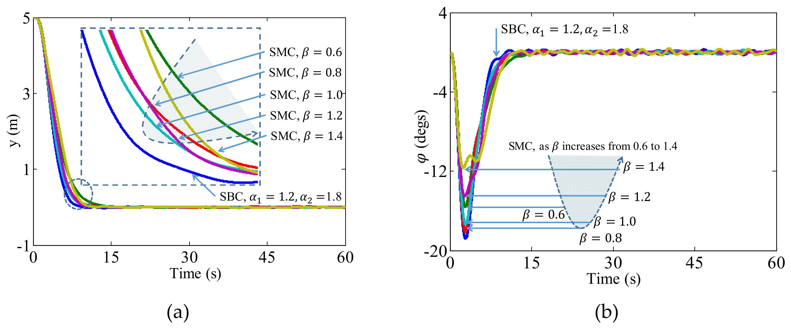
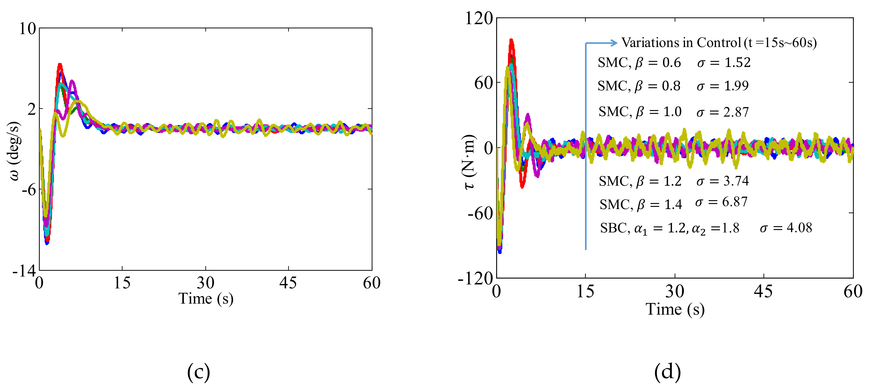
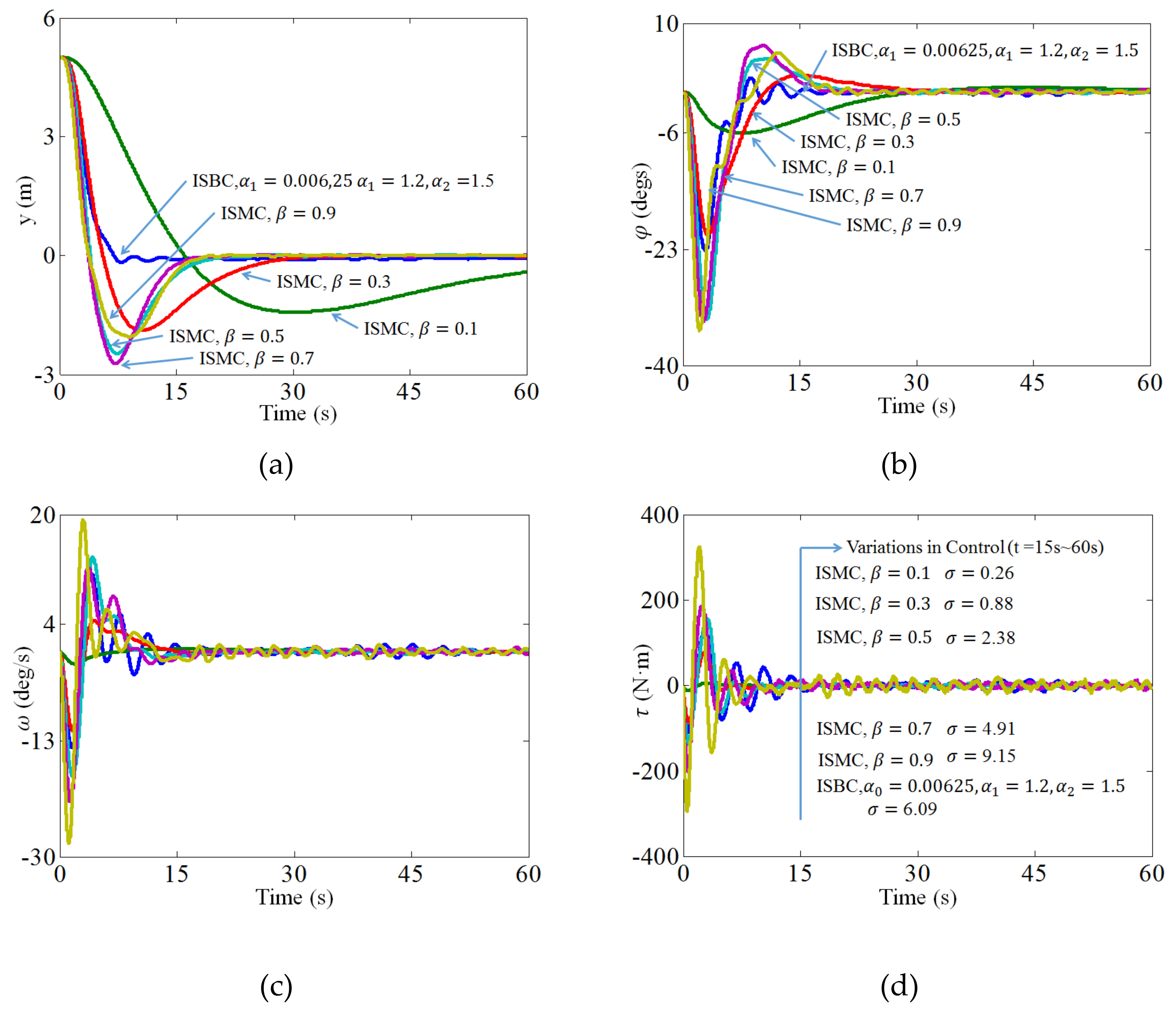
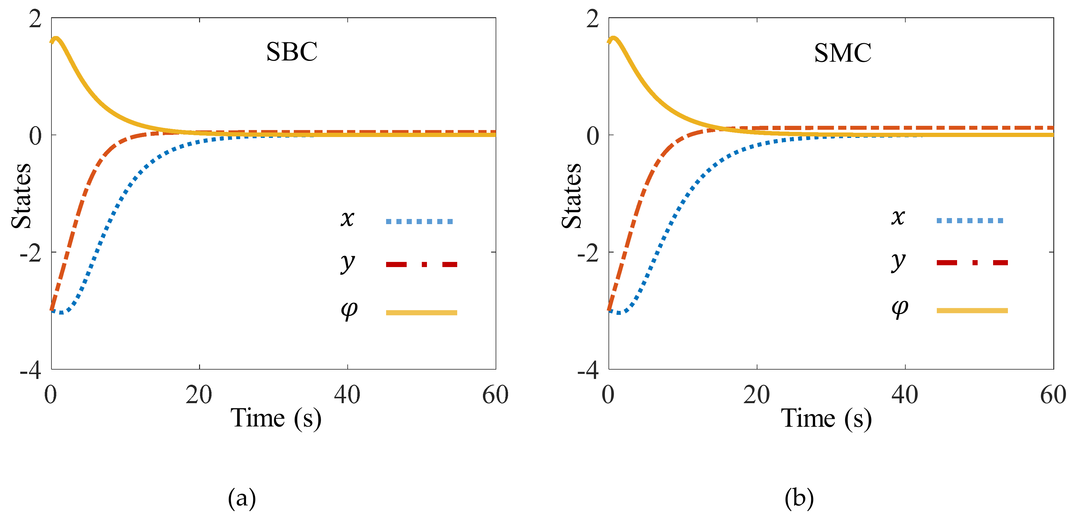
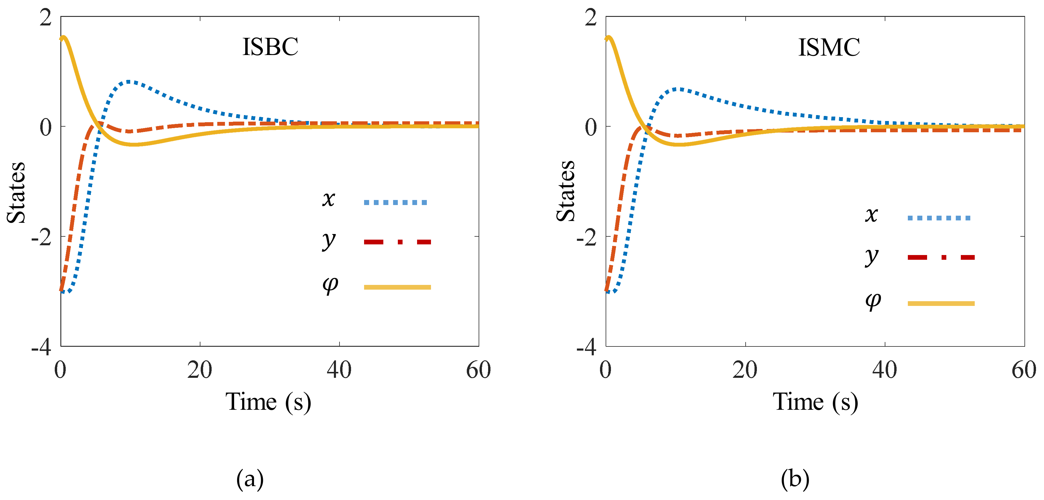
5. Simulation Results

To validate the performance of the proposed SBC and ISBC, two cases of control of an autonomous underwater vehicle (AUV) are provided, including (1) Case I: line following cruise control (SISO system) and Case II: planar motion control (MIMO system). As shown in Figure 1, the motion of the AUV in XY plane is controlled by the thrust force $F$ and steering torque $\tau$. The position of the AUV is represented by the location of its center of mass $\left(x,y\right)$, $V$ is the speed, and $\phi$ is the heading angle.

Case I: SISO system control—line following cruise control of the AUV

This line following cruise tracking control problem simulates an application of using an AUV for sea floor mapping or searching, where the AUV scans a field with a constant speed following a zig-zag pattern. Here, we assume that speed control is handled by another controller, such that the system is an SISO system. The goal of cruise tracking control is to drive the AUV to follow a straight line at a cruise speed $V_0$. More specifically, if we desire that the AUV cruises along the x-axis, the goal is to drive $y$ to zero in a finite time, while also converging to the cruise speed $V_0$. The associated system dynamics are given by:

$$\left\{\begin{array}{c}\dot{x}=V_{0}cos\phi \hfill \\ \dot{y}=V_{0}sin\phi \hfill \\ \dot{\phi }=\omega \hfill \\ J\dot{\omega }=\tau \hfill \end{array}\right.$$

(43)

where $\omega$ is the angular rate and $J$ is the mass moment of inertia of the AUV. Since this is a SISO system, we can follow Theorem 1 to design the controller. First, the system is converted to the canonical form by using input-output linearization:

$$\left\{\begin{array}{c}{x}_1=y\hfill \\ x_2=\dot{y}=V_{0}sin\phi \hfill \\ x_3=y^{\left(2\right)}=V_{0}cos\phi \dot{\phi }=V_0\omega cos\phi \hfill \\ y^{\left(3\right)}=-V_0{\omega }^{2}sin\phi +\frac{1}{J}{V}_{0}cos\phi \tau \hfill \end{array}\right.$$

(44)

Then, the equivalent dynamics are given as:

$$\left\{\begin{array}{c}{\dot{x}}_1=x_2\hfill \\ {\dot{x}}_2=x_3\hfill \\ {\dot{x}}_3=f\left(x\right)+g\left(x\right)u\hfill \end{array}\right.$$

(45)

where $f\left(x\right)=-V_0\omega sin\phi \dot{\phi }$, $g\left(x\right)=\frac{1}{J}{V}_{0}cos\phi$ and $u=\tau$.

Secondly, we define $s_{SBC}$ and $d_{SBC}$ as follows:

$$\left\{\begin{array}{c}{s}_{SBC}=x_3+{\alpha }_2{x}_2+{\alpha }_1{x}_1\hfill \\ d_{SBC}={\alpha }_2{x}_3+{\alpha }_1{x}_2\hfill \end{array}\right.$$

(46)

Correspondingly, for ISBC, we have:

$$\left\{\begin{array}{c}{s}_{ISBC}=x_3+{\alpha }_2{x}_2+{\alpha }_1{x}_1+{\alpha }_0{x}_0\hfill \\ d_{ISBC}={\alpha }_2{x}_3+{\alpha }_1{x}_2+{\alpha }_0{x}_1\hfill \end{array}\right.$$

(47)

and, for SMC and Integral sliding mode control (ISMC)

$$\left\{\begin{array}{c}{s}_{SMC}=x_3+2\beta x_2+{\beta }^2{x}_1\hfill \\ d_{SMC}=2\beta x_3+{\beta }^2{x}_2\hfill \end{array}\right.$$

(48)

$$\left\{\begin{array}{c}{s}_{ISMC}=x_3+3\beta x_2+3{\beta }^2{x}_1+{\beta }^3{x}_0\hfill \\ d_{ISMC}=3\beta x_3+3{\beta }^2{x}_2+{\beta }^3{x}_1\hfill \end{array}\right.$$

(49)

Then, the control laws share the same form:

$$u=\frac{1}{\widehat{g}\left(x\right)}\left[-\widehat{f}\left(x\right)-{\widehat{d}}_{\left(*\right)}\left(x\right)-k sgn(s_{\left(*\right)}\right)]$$

(50)

where $\widehat{f}\left(x\right)$, $\widehat{g}\left(x\right)$, and $\widehat{d}\left(x\right)$ are nominal functions of $f\left(x\right)$, $g\left(x\right)$, and $d\left(x\right)$, respectively; and the subscript ${}_{\left(*\right)}$ can be one of the four choices of $\left\{{}_{SBC},{ }_{ISBC},{ }_{SMC}{,}_{ISMC}\right\}$.

The matching condition can be quantified through Monte Carlo simulation and experimental tests. The control input is given by Equation (12), where $s$ and $d$ are chosen according to the specific control algorithm to be used (i.e., if SBC is chosen, $s=s_{SBC}$ and $d=d_{SBC}$).

The four controllers were compared under the same testing scenario where the mass is $m$ = 200 kg, moment of inertia is $J$ = 450 kg·m², cruise speed is $V_0=$4 m/s, and the vehicle is controlled to track the x-axis from the initial position of $\left[x_0,y_0\right]=$ [0, 5] m. The noise in position, angle, and angular rate are assumed to be zero-mean and Gaussian with a standard deviation of 0.1 m, 1 degree, and 0.01 degree/s, respectively. Note that all noise is assumed to be bounded within a range of $\pm 3\sigma$. A MATLAB/Simulink model is developed, and the results are shown in Figure 2 and Figure 3.

Figure 2 shows the performance comparison of the SBC and SMC controllers, where (a), (b), (c) and (d) are the y-position, heading angle, angular rate, and control signal, respectively. To provide a complete performance comparison, results for SMCs with different control parameters (i.e., $\beta =$ 0.6, 0.8, 1.0, 1.2, and 1.4) are produced to compare with the proposed SBC (${\alpha }_1=$ 1.2, and ${\alpha }_2=$1.8). It can be seen from Figure 2a that SBC can drive the AUV to approach zero in a shorter time compared to SMC. As the parameter $\beta$ of SMC increases from 0.6 to 1.4, the performance becomes similar to the SBC before diverging from it. The rise time under these six controls are given in

Table 1. Rise times of SBC and SMC.

Rise Time	C0	C1	C2	C3	C4	C5
$t_r$	6.73 s	9.61 s	8.10 s	7.66 s	7.96 s	8.65 s

Note: C0 = SBC, C1, C2, …, C5 = SMC with $\beta =$ 0.6, 0.8, …, 1.4.

. It can be seen that the SBC has the shortest rise time of 6.73 s, while the quickest rise time of the five SMCs is 7.66 s.

The performance changes as $\beta$ increases can be analyzed from the variations in the coefficients of $s_{SMC}$ and $d_{SMC}$. Recall that $x_1=y$ and $x_2=\dot{y}$, where the coefficients as shown in Equation (16) correspond to the proportional and derivative gain in PID controller design. Since the two coefficients ${\beta }^2$ and $2\beta$ are dependent, the performance of the controller is also restricted to a certain extent due to the freedom in parameter selection being reduced from 2 to 1.

Figure 3 shows the performance comparison of the SBC and SMC controllers, where (a), (b), (c) and (d) are the y-position, heading angle, angular rate, and control signal, respectively. To provide a complete performance comparison, results of ISMCs with different control parameters (i.e., $\beta =$0.1, 0.3, 0.5, 0.7, and 0.9) are produced to compare with the proposed SBC (${\alpha }_0=$0.0625, ${\alpha }_1=$ 1.2, and ${\alpha }_2=$1.5). It can be seen from Figure 2a that ISBC can drive the AUV to reach steady state in a much shorter time of 8.9 seconds compared to ISMCs. The performance indices, including rise time $t_r$, settling time $t_s$, peak time $t_p$, and overshot $\sigma \%$ are summarized in

Table 2. Performance comparison between ISBC and ISMC.

System Response	C0	C1	C2	C3	C4	C5
tr	6.28 s	15.14 s	5.32 s	3.83 s	3.52 s	3.52 s
ts	8.90 s	> 60 s	30.53 s	21.29 s	17.01 s	18.25 s
ts	8.01 s	30.21 s	10.64 s	7.50 s	7.15 s	8.97 s
σ%	3.5%	28.6%	37.8%	49.5%	54.6%	40.9%

Note: C0 = ISBC, C1, C2, …, C5 = ISMC with $\beta =$ 0.1, 0.3, …, 0.9.

. It can be seen that the ISBC has the best performance with respect to the rising time, settling time, peak time, and overshoot. Due to the dependency in the control gains, ISMCs have difficulty in achieving better performances; i.e., as $\beta$ increases (from C1 to C5 in Table 2), the settling time, rising time, peak time, and overshoot first decrease then increase.

It can be seen from Figure 3b,c that, during the control process, ISBC has the smallest variation in heading angle and angular rate compared to ISMCs. Figure 3d shows that all the controllers can maintain the desired states with relatively small variations in control signals with a standard deviation of less than 10 N.

From the comparison in these two experiments, we can see that the dependency in control gain selection simplifies the controller tuning, meanwhile the dependency also limits the performance of the control system.

Case II: MIMO system—planar motion control of the AUV

Planar motion control of the AUV is used to show the effectiveness of the proposed controller design for MIMO systems. The dynamics of planar motion of the AUV is given as follows:

$$\left\{\begin{array}{c}\dot{x}=Vcos\phi \hfill \\ \dot{y}=Vsin\phi \hfill \\ \dot{\phi }=\omega \hfill \\ m\dot{V}=F-c{V}^2\hfill \\ J\dot{\omega }=\tau \hfill \end{array}\right.$$

(51)

where $c$ is the drag coefficient and the drag force is $c{V}^2$. Since this is a MIMO system, we can follow Theorem 2 to design the controller. First, the system is converted to the canonical form by using input-output linearization.

Let ${\mathit{x}}_1=\left\{\begin{array}{c}x\hfill \\ y\hfill \\ \phi \hfill \end{array}\right\}$, ${\mathit{x}}_2=\left\{\begin{array}{c}\dot{x}\hfill \\ \dot{\begin{array}{c}y\hfill \\ \dot{\phi }\hfill \end{array}}\hfill \end{array}\right\}=\left\{\begin{array}{c}\begin{array}{c}Vcos\phi \hfill \\ Vsin\phi \hfill \end{array}\hfill \\ \omega \hfill \end{array}\right\}$, then ${\dot{\mathit{x}}}_2={\left\{\begin{array}{c}x\hfill \\ y\hfill \\ \phi \hfill \end{array}\right\}}^{\left(2\right)}=\left\{\begin{array}{c}\frac{1}{m}\left(F-c{V}^2\right)cos\phi -V\omega sin \phi \hfill \\ \frac{1}{m}\left(F-c{V}^2\right)sin\phi +V\omega cos\phi \hfill \\ \frac{1}{J}\tau \hfill \end{array}\right\}$ and the equivalent dynamics is given as

$$\left\{\begin{array}{c}{\dot{\mathit{x}}}_1={\mathit{x}}_2\hfill \\ {\dot{\mathit{x}}}_2=\mathit{f}\left(\mathit{x}\right)+\mathit{g}\left(\mathit{x}\right)\mathit{u}\hfill \end{array}\right.$$

(52)

where $\mathit{f}\left(\mathit{x}\right)=\left\{\begin{array}{c}-\frac{1}{m}c{V}^{2}cos\phi -V\omega sin \phi \hfill \\ -\frac{1}{m}c{V}^{2}sin\phi +V\omega cos\phi \hfill \\ 0\hfill \end{array}\right\}$, $\mathit{g}\left(\mathit{x}\right)=\left[\begin{array}{cc}\frac{1}{m}cos\phi \hfill & 0\hfill \\ \frac{1}{m}sin\phi \hfill & 0\hfill \\ 0\hfill & \frac{1}{J}\hfill \end{array}\right]$, and $\mathit{u}=\left\{\begin{array}{c}F\hfill \\ \tau \hfill \end{array}\right\}$. Secondly, we can define $\mathit{s}$ and $\mathit{d}$ functions for SBC as follows

$$\left\{\begin{array}{c}{\mathit{s}}_{SBC}={\mathit{x}}_2+{\mathit{\alpha }}_1{\mathit{x}}_1\hfill \\ {\mathit{d}}_{SBC}={\mathit{\alpha }}_1{\mathit{x}}_2\hfill \end{array}\right.$$

(53)

Correspondingly, for ISBC, we have:

$$\left\{\begin{array}{c}{\mathit{s}}_{ISBC}={\mathit{x}}_2+{\alpha }_1{x}_1+{\mathit{\alpha }}_0{\mathit{x}}_0\hfill \\ {\mathit{d}}_{ISBC}={\mathit{\alpha }}_1{\mathit{x}}_2+{\mathit{\alpha }}_0{\mathit{x}}_1\hfill \end{array}\right.$$

(54)

and, for SMC and ISMC,

$$\left\{\begin{array}{c}{\mathit{s}}_{SMC}={\mathit{x}}_3+2\beta {\mathit{x}}_2+{\beta }^2{\mathit{x}}_1\hfill \\ {\mathit{d}}_{SMC}=2\beta {\mathit{x}}_3+{\beta }^2{\mathit{x}}_2\hfill \end{array}\right.$$

(55)

$$\left\{\begin{array}{c}{\mathit{s}}_{ISMC}={\mathit{x}}_3+3\beta {\mathit{x}}_2+3{\beta }^2{\mathit{x}}_1+{\beta }^3{\mathit{x}}_0\hfill \\ {\mathit{d}}_{ISMC}=3\beta {\mathit{x}}_3+3{\beta }^2{\mathit{x}}_2+{\beta }^3{\mathit{x}}_1\hfill \end{array}\right.$$

(56)

Then, the control laws share the same form

$$\mathit{u}=\widehat{\mathit{g}}{\left(\mathit{x}\right)}^{+}\left[-\widehat{\mathit{f}}\left(\mathit{x}\right)-{\widehat{\mathit{d}}}_{\left(*\right)}\left(\mathit{x}\right)-\mathit{k}sgn\left({\mathit{s}}_{\left(*\right)}\right)\right]$$

(57)

where ${}_{\left(*\right)}$ can be one of the four choices $\left\{{}_{SBC},{ }_{ISBC},{ }_{SMC}{,}_{ISMC}\right\}$ given in Equations (53)–(56).

The matching conditions and AUV specifications are the same as those for Case I, while the speed of the AVU is treated as a state variable. The control parameters are listed in

Table 3. Control parameter selection.

Control Method	Parameters
SMC	$\beta = 0.2$
SBC	${\alpha }_1=0.2\times \left[1;0.9;1\right]$
ISMC	$\beta = 0.2$
ISBC	${\alpha }_1=0.4\times \left[1.1;1;1\right] and {\alpha }_0=0.04\times \left[1.25;1;1\right]$

and simulation results are shown in Figure 4 and Figure 5. The initial conditions are given as $x\left(0\right)=-3m, y=-3m, and \phi \left(0\right)=\frac{\pi }{2}.$

Figure 4 shows the performance comparison of the SBC and SMC. It can be seen from that SBC can control the AUV to approach zero in a shorter time compared to SMC. The rise time is given in

Table 4. Rise time of SBC and SMCs.

Rise Time	SMC	SBC
$t_r \left(x,y,\phi \right)$	13.01, 7.73, 11.21 (s)	11.71, 7.18, 10.25 (s)

. Moreover, SBC allows us to adjust the performance of each state by tuning the corresponding control parameters. By comparing Figure 4a,b it can also be seen that the steady state error in y direction in SBC is much smaller than that for SMC. This is achieved by choosing a different control parameter for y direction as indicated in Table 3. Figure 5 shows the performance comparison of the ISBC and ISMC. By choosing a different control parameter for x direction in ${\alpha }_0$, the settling time of state x is reduced from 41.22 s for ISMC to 34.72 s for ISBC.

By comparing the controller performance for the two cases, it can be seen that the proposed SBC and ISBC can achieve better performance comparing to SMC and ISMC. This improvement is achieved by flexibility in control parameter selections. Similar strategies can be used for controller parameter selection for all these four different controllers. Additionally, if ${\alpha }_1=\beta \left\{1;1;1\right\}$, SBC and SMC two controllers will be equivalent if ${\alpha }_1=\beta \left\{1;1;1\right\}$. Similarly, for ISMC and ISBC, if ${\alpha }_1=2\beta \left\{1;1;1\right\}, \mathrm{and} {\alpha }_0={\beta }^2\left\{1;1;1\right\}$, these two controllers will be equivalent.

6. Conclusions

In this paper, a sliding mode control in the backstepping framework (SBC) was proposed for a class of nonlinear systems. The comparison between the SBC and sliding mode control was discussed by comparing dependency in the control gains. An example of cruise control of an unmanned underwater vehicle was given to show the effectiveness of the controller. It was found that the proposed controller is able to achieve better control performance due to its advantages in the flexibility of control gain selection and simplicity in control law formulation when considering useful nonlinearities.

References

1. Khalil, H. Nonlinear Systems, 3rd ed.; Prentice Hall: Upper Saddle River, NJ, USA, 2001. [Google Scholar]
2. Chen, M.; Ge, S.S.; Ren, B. Robust attitude control of helicopters with actuator dynamics using neural networks. IET Control Theory Appl. 2010, 4, 2837–2854. [Google Scholar] [CrossRef] [Green Version]
3. Ki-Seok, K.; Youdan, K. Robust backstepping control for slew maneuver using nonlinear tracking function. IEEE Trans. Control Syst. Technol. 2003, 11, 822–829. [Google Scholar] [CrossRef] [Green Version]
4. Mou, C.; Bin, J. Robust bounded control for uncertain flight dynamics using disturbance observer. J. Syst. Eng. Electron. 2014, 25, 640–647. [Google Scholar]
5. Azinheira, J.; Moutinho, A. Hover Control of an UAV with Backstepping Design Including Input Saturations. IEEE Trans. Control Syst. Technol. 2008, 16, 517–526. [Google Scholar] [CrossRef]
6. Chen, M.; Ge, S.; How, B.V.; Choo, Y.S. Robust adaptive position mooring control for marine vessels. IEEE Trans. Control Syst. Technol. 2013, 21, 395–409. [Google Scholar] [CrossRef]
7. Fossen, T.; Grovlen, A. Nonlinear output feedback control of dynamically positioned ships using vectorial observer backstepping. IEEE Trans. Control Syst. Technol. 1998, 6, 121–128. [Google Scholar] [CrossRef]
8. Ghommam, J.; Mnif, F.; Benali, A.; Derbel, N. Asymptotic Backstepping Stabilization of an Underactuated Surface Vessel. IEEE Trans. Control Syst. Technol. 2006, 14, 1150–1157. [Google Scholar] [CrossRef]
9. Kwan, C.; Lewis, F. Robust backstepping control of induction motors using neural networks. IEEE Trans. Neural Netw. 2000, 11, 1178–1187. [Google Scholar] [CrossRef]
10. Drid, S.; Naït-Saïd, M.-S.; Tadjine, M. Robust backstepping vector control for the doubly fed induction motor. IET Control Theory Appl. 2007, 1, 861–868. [Google Scholar] [CrossRef]
11. Lin, F.-J.; Lee, C.-C. Adaptive backstepping control for linear induction motor drive to track periodic references. IEE Proc. Electr. Power Appl. 2000, 147, 449. [Google Scholar] [CrossRef]
12. Zhao, D.; Gao, F.; Li, S.; Zhu, Q. Robust finite-time control approach for robotic manipulators. IET Control Theory Appl. 2010, 4, 1–15. [Google Scholar] [CrossRef] [Green Version]
13. Yoo, S.J.; Park, J.B.; Choi, Y.H. Adaptive Output Feedback Control of Flexible-Joint Robots Using Neural Networks: Dynamic Surface Design Approach. IEEE Trans. Neural Netw. 2008, 19, 1712–1726. [Google Scholar]
14. Shojaei, K.; Shahri, A. Adaptive robust time-varying control of uncertain non-holonomic robotic systems. IET Control Theory Appl. 2012, 6, 90. [Google Scholar] [CrossRef]
15. Zhou, H.; Liu, Z. Vehicle Yaw Stability-Control System Design Based on Sliding Mode and Backstepping Control Approach. IEEE Trans. Veh. Technol. 2010, 59, 3674–3678. [Google Scholar] [CrossRef]
16. Shen, P.-H.; Lin, F.-J. Intelligent backstepping sliding-mode control using RBFN for two-axis motion control system. IEE Proc. Electr. Power Appl. 2005, 152, 1321. [Google Scholar] [CrossRef]
17. Liu, Z.; Jia, X. Novel backstepping design for blended aero and reaction-jet missile autopilot. J. Syst. Eng. Electron. 2008, 19, 148–153. [Google Scholar]
18. Hua, C.; Liu, P.X.; Guan, X.; Liu, P.; Liu, P. Backstepping Control for Nonlinear Systems With Time Delays and Applications to Chemical Reactor Systems. IEEE Trans. Ind. Electron. 2009, 56, 3723–3732. [Google Scholar]
19. Mazenc, F.; Bliman, P.-A. Backstepping Design for Time-Delay Nonlinear Systems. IEEE Trans. Autom. Control 2006, 51, 149–154. [Google Scholar] [CrossRef] [Green Version]
20. Shiromoto, H.S.; Andrieu, V.; Prieur, C. Relaxed and Hybridized Backstepping. IEEE Trans. Autom. Control 2013, 58, 3236–3241. [Google Scholar] [CrossRef] [Green Version]
21. Zhang, Y.; Fidan, B.; Ioannou, P.A. Backstepping control of linear time-varying systems with known and unknown parameters. IEEE Trans. Autom. Control 2003, 48, 1908–1925. [Google Scholar] [CrossRef]
22. Cheng, C.-C.; Su, G.-L.; Chien, C.-W. Block backstepping controllers design for a class of perturbed non-linear systems with m blocks. IET Control Theory Appl. 2012, 6, 2021–2030. [Google Scholar] [CrossRef]
23. Zhou, J.; Zhang, C.; Wen, C. Robust Adaptive Output Control of Uncertain Nonlinear Plants with Unknown Backlash Nonlinearity. IEEE Trans. Autom. Control 2007, 52, 503–509. [Google Scholar] [CrossRef]
24. Wang, Z.; Ge, S.; Lee, T. Robust adaptive neural network control of uncertain nonholonomic systems with strong nonlinear drifts. IEEE Trans. Syst. Man Cybern. Part B Cybern. 2004, 34, 2048–2059. [Google Scholar] [CrossRef] [PubMed]
25. Wang, J.; Hu, J. Robust adaptive neural control for a class of uncertain non-linear time-delay systems with unknown dead-zone non-linearity. IET Control Theory Appl. 2011, 5, 1782–1795. [Google Scholar] [CrossRef]
26. Mazenc, F.; Ito, H. Lyapunov technique and backstepping for nonlinear neutral systems. IEEE Trans. Autom. Control 2013, 58, 512–517. [Google Scholar] [CrossRef]
27. Hyeongcheol, L. Robust adaptive fuzzy control by backstepping for a class of MIMO nonlinear systems. IEEE Trans. Fuzzy Syst. 2011, 19, 265–275. [Google Scholar]
28. Wang, H.; Chen, B.; Liu, X.; Liu, K.; Lin, C. Robust Adaptive Fuzzy Tracking Control for Pure-Feedback Stochastic Nonlinear Systems With Input Constraints. IEEE Trans. Cybern. 2013, 43, 2093–2104. [Google Scholar] [CrossRef]
29. Tong, S.-C.; He, X.-L.; Zhang, H.-G. A Combined Backstepping and Small-Gain Approach to Robust Adaptive Fuzzy Output Feedback Control. IEEE Trans. Fuzzy Syst. 2009, 17, 1059–1069. [Google Scholar] [CrossRef]
30. Wai, R.; Lee, J. Robust levitation control for linear maglev rail system using fuzzy neural network. IEEE Trans. Control Syst. Technol. 2009, 17, 4–14. [Google Scholar]
31. Shafiei, S.E.; Soltanpour, M.R. Robust neural network control of electrically driven robot manipulator using backstepping approach. Int. J. Adv. Robot. Syst. 2009, 6, 285–292. [Google Scholar] [CrossRef]
32. Kwan, C.; Lewis, F. Robust backstepping control of nonlinear systems using neural networks. IEEE Trans. Syst. Man Cybern. Part A Syst. Hum. 2000, 30, 753–766. [Google Scholar] [CrossRef]
33. Chen, M.; Ge, S.S.; How, B. Robust Adaptive Neural Network Control for a Class of Uncertain MIMO Nonlinear Systems with Input Nonlinearities. IEEE Trans. Neural Netw. 2010, 21, 796–812. [Google Scholar] [CrossRef] [PubMed]
34. Kuljaca, O.; Swamy, N.; Lewis, F.; Kwan, C. Design and implementation of industrial neural network controller using backstepping. IEEE Trans. Ind. Electron. 2003, 50, 193–201. [Google Scholar] [CrossRef]
35. Hsu, C.-F.; Lin, C.-M.; Lee, T.-T. Wavelet Adaptive Backstepping Control for a Class of Nonlinear Systems. IEEE Trans. Neural Netw. 2006, 17, 1175–1183. [Google Scholar]
36. Wai, R.-J.; Chang, H.-H. Backstepping Wavelet Neural Network Control for Indirect Field-Oriented Induction Motor Drive. IEEE Trans. Neural Netw. 2004, 15, 367–382. [Google Scholar] [CrossRef]
37. Hua, C.; Guan, X.; Shi, P. Robust backstepping control for a class of time delayed systems. IEEE Trans. Autom. Control 2005, 50, 894–899. [Google Scholar]
38. Ezal, K.; Pan, Z.; Kokotovic, P. Locally optimal and robust backstepping design. IEEE Trans. Autom. Control 2000, 45, 260–271. [Google Scholar] [CrossRef]
39. French, M. An analytical comparison between the nonsingular quadratic performance of robust and adaptive backstepping designs. IEEE Trans. Autom. Control 2002, 47, 670–675. [Google Scholar] [CrossRef]
40. Sabanovic, A. Variable structure systems with sliding modes in motion vontrol-a survey. IEEE Trans. Ind. Inform. 2011, 7, 212–223. [Google Scholar] [CrossRef]
41. Young, K.; Utkin, V.; Ozguner, U. A control engineer’s guide to sliding mode control. IEEE Trans. Control Syst. Technol. 1999, 7, 328–342. [Google Scholar] [CrossRef] [Green Version]
42. Slotine, J.J.; Li, W. Applied Nonlinear Control; Prentice-Hall International: Upper Saddle River, NJ, USA, 1991. [Google Scholar]
43. Kachroo, P.; Tomizuka, M. Chattering reduction and error convergence in the sliding-mode control of a class of nonlinear systems. IEEE Trans. Autom. Control 1996, 41, 1063–1068. [Google Scholar] [CrossRef] [Green Version]
44. Fallaha, C.J.; Saad, M.; Kanaan, H.Y.; Al-Haddad, K. Sliding-mode robot control with exponential reaching law. IEEE Trans. Ind. Electron. 2011, 58, 600–610. [Google Scholar] [CrossRef]
45. Acary, V.; Brogliato, B.; Orlov, Y.V. Chattering-rree digital sliding-mode control with state observer and disturbance rejection. IEEE Trans. Autom. Control 2012, 57, 1087–1101. [Google Scholar] [CrossRef] [Green Version]
46. Lin, C.-K.; Liu, T.-H.; Wei, M.-Y.; Fu, L.-C.; Hsiao, C.-F. Design and implementation of a chattering-free non-linear sliding-mode controller for interior permanent magnet synchronous drive systems. IET Electr. Power Appl. 2012, 6, 332. [Google Scholar] [CrossRef]
47. Lin, F.-J.; Shen, P.-H.; Hsu, S.-P. Adaptive backstepping sliding mode control for linear induction motor drive. IEE Proc. Electr. Power Appl. 2002, 149, 184. [Google Scholar] [CrossRef]
48. Skjetne, R.; Fossen, T. On integral control in backstepping: Analysis of different techniques. In Proceedings of the 2004 American Control Conference, Boston, MA, USA, 30 June–2 July 2004; Volume 2, pp. 1899–1904. [Google Scholar]
49. Xiao, L.; Zhu, Y. Passivity-based integral sliding mode active suspension control. In Proceedings of the 19th World Congress of the International Federation of Automatic Control, Cape Town, South Africa, 24–29 August 2014. [Google Scholar]
50. Bartolini, G.; Ferrara, A.; Usai, E. Chattering avoidance by second-order sliding mode control. IEEE Trans. Autom. Control 1998, 43, 241–246. [Google Scholar] [CrossRef]
51. Kurode, S.; Spurgeon, S.K.; Bandyopadhyay, B.; Gandhi, P.S. Sliding mode control for slosh-free motion using a nonlinear sliding surface. IEEE/ASME Trans. Mechatron. 2013, 18, 714–724. [Google Scholar] [CrossRef] [Green Version]
52. Leung, F.; Wong, L.; Tam, P. Algorithm for eliminating chattering in sliding mode control. Electron. Lett. 1996, 32, 599. [Google Scholar] [CrossRef]
53. Kachroo, P. Existence of solutions to a class of nonlinear convergent chattering-free sliding mode control systems. IEEE Trans. Autom. Control 1999, 44, 1620–1624. [Google Scholar] [CrossRef] [Green Version]
Figure 1. Sketch of an autonomous underwater vehicle.
Jmse 07 00452 g001
Figure 2. Performance comparison of SBC and SMC. (a), (b), (c) and (d) are the y-position, heading angle, angular rate, and control signal.
Jmse 07 00452 g002aJmse 07 00452 g002b
Figure 3. Performance comparison of ISBC and ISMC.
Jmse 07 00452 g003
Figure 4. Performance comparison of SBC (a) and SMC (b).
Jmse 07 00452 g004
Figure 5. Performance comparison of ISBC (a) and ISMC (b).
Jmse 07 00452 g005