1. Introduction
Interactions of waves with currents and bathymetry constitute interesting problems, with an important effect on significant nearshore coastal processes and in finding useful applications to coastal and harbor engineering. Especially when the currents vary with depth, as observed in cases of strong tidal currents [
1] or wind-driven currents [
2], the presence of vorticity should be taken into account in modelling the propagation of water waves. This is important in designing efficient energy production devices and more generally in coastal zone management. This is especially true in coastal and onshore regions [
3,
4], where additional factors due to bathymetry variations and flow termination at the shoreline contribute to increasing the complexity of the flow. Furthermore, the strong reflection of waves interacting with undular bottom topography, which has important effects on coastal dynamics, adds to the complexity of the considered problems and requires the development and validation of a special class of models to represent the involved physical processes.
In cases when vorticity is present in the current flow, the wave-vorticity interaction can have a significant influence on water-wave dynamics. This is important, especially in the case of coastal currents which vary slowly, horizontally, but are characterized by vertical gradients, as in the case of tidal currents and in oceanic conditions where the vertical variation of the current might be significant; see, e.g., [
1,
4]. Several authors developed models to treat the effects of shear current on water wave propagation; see, e.g., [
5,
6,
7]. In the recent work by Quinn, et al. [
8], a wave action conservation equation is presented with application to slowly varying bathymetry and arbitrary shear current. However, in its present form, this model is not directly applicable to wave systems containing a forward propagating and a back-propagating component that could be excited by resonant reflection. More recently, experimental and numerical studies on wave–current interaction have been presented by Musumeci et al. [
9] and Viviano et al. [
10,
11].
Moreover, simplified models based on the assumption of linear vertical current profile (e.g., Thomas and Klopman [
4], Ch.3.1), corresponding to locally constant vorticity, have been developed, supporting the study of the effects of vertically uniform shear on the dispersive properties of the waves; see, [
5,
12,
13]. Additional effects of bathymetric inhomogeneities on propagation and scattering phenomena have been considered by Brink-Kjaer and Jonsson [
14] and Brink-Kjaer [
15]. In simplified 2D flow problems in the vertical plane, the wave flow can be approximated in the framework of potential formulation, however, as clearly demonstrated by Ellingsen [
16], in the case of general 3D problems and the interaction of oblique waves with vertically sheared current, the latter assumption turns out to be over-restrictive.
In recent works concerning the wave–current–seabed interaction problem, with application to wave scattering by non-homogeneous, vertically linear sheared current over general bathymetry extended mild-slope equations by Touboul et al. [
17] and coupled-mode systems by Belibassakis et al. [
18] has been derived based on the potential approximation of wave flow. The latter models are applicable to 2D flow problems with constant vorticity and approximately applicable to 2D problems characterized by sufficiently slowly varying vorticity. More details concerning this fact and additional limitations are discussed in
Appendix A. In the above works, the scattered wave potential is represented by a series of local vertical modes containing the propagating and evanescent modes plus additional terms accounting for the satisfaction of the boundary conditions on a sloping seabed. Using the above representation, in conjunction with a variational principle, a coupled system of differential equations on the horizontal plane is derived, with respect to the unknown modal amplitudes. In the case of no shear, the above coupled-mode system reduces exactly to the one developed by Belibassakis et al. [
19] for the propagation of small-amplitude water waves over variable bathymetry regions in the presence of horizontally varying ambient currents. Furthermore, if only the propagating mode is maintained in the local-mode series, the present coupled-mode system naturally reduces to a simplified one-equation model for wave propagation, taking both current and vorticity effects into account, thus saving a lot of computational burden when such a simplification is permitted. The latter model is found to be compatible with the extended mild-slope equation for surface waves interacting with a vertically sheared current recently derived and studied by Touboul et al. [
17]. Furthermore, in the case of no current, it reduces exactly to the modified mild-slope equation, presented by Massel [
20] and Chamberlain and Porter [
21].
In this work, the applicability of the extended mild-slope system (MMS) derived by Touboul et al. [
17] and of the enhanced version by Belibassakis et al. [
18] is examined in the case of Bragg scattering of waves in the presence of opposing shearing currents. It is shown that the MMS is able to provide quite good predictions in the case of Bragg scattering of waves over sinusoidal bathymetry without a current, however, it fails to accurately predict the resonant frequency in the case of a current, although it still provides reasonable values of the reflected wave amplitudes. In order to resolve the above mismatch, a two-equation mild-slope system (CMS2) is derived from the variational principle presented in Belibassakis et al. [
18], assuming representation of the wave potential as a superposition of forward- and back-propagating modes. The latter system is shown to provide more accurate predictions concerning both the resonant frequency and the amplitude of the reflection coefficient.
2. Experimental Results
For the validation of the coupled-mode system, comparisons with experimental data are presented in the case of normally incident waves propagating over a trapezoidal bar, seated on a flat horizontal bottom in the presence of an opposing vertically sheared current. The shear is obtained by means of an appropriately designed screen, in order for the current to be numerically modelled by using a linear profile in depth,
where
denotes the surface current at
z = 0, where
z denotes the vertical coordinate positive upwards, and
denotes the locally constant shear in the vertical water column at any
x-position. The experiments were carried out in a 10 m long, 0.3 m wide and 0.50 m high wave flume (SeaTech, University of Toulon, La Garde, France). The current was injected in the channel by a hydraulic pump with a prescribed discharge rate of 0.01 m
3/s. At the downstream end of the channel, regular waves were generated by means of an electromagnetic piston-type wavemaker. At the upstream end, a slopping beach was used to absorb the wave. Both the wave-maker paddle and the beach were elevated to let the water flow in the channel. The experimental arrangement and details are presented in
Figure 1.
For the experiments, the water depth was 0.305 m and experimental data were recorded for wave frequencies ranging from 0.65 Hz to 1.3 Hz with amplitudes between 1–2 cm ensuring small wave steepness both without current and with a vertically sheared current. In this case, the reflected component is small and both the mild-slope model and the coupled-mode system provide good predictions in comparison with experimental measurements. More details are available in [
18].
The case of stronger reflection in resonant conditions of waves over sinusoidal bottom profiles, in the presence of an opposing shear current, is experimentally and theoretically studied by Laffite et al. [
22]. The mean depth in the experiments is
h = 0.22 m and the bottom profile consists of 10 sinusoidal ripples of amplitude
ha = 0.035 m. The bathymetry is given by
and the wavelength of the sinusoidal bottom undulations is
. A schematic presentation of the experimental setup is presented in
Figure 2. Three synchronized, resistive wave probes were operated using a 128 Hz sampling rate within this study. They were devoted to the computation of the reflexion coefficient, upwave of the sinusoidal bottom. The data presented in the following are based on a three-probes method analysis, as described in detail by Rey et al. [
23]. Current measurements were based on Vectrino™ acoustic doppler velocimeters, developed by the Nortek Company, Rud, Norway. Their locations are also presented in
Figure 2. These acoustic Doppler velocimeters recorded data at a sampling rate of 200 Hz, and were mounted on vertically moving carriages, for the purpose of obtaining precise vertical profiles for the mean current velocities. These profiles, obtained by averaging the data, are presented in
Figure 3.
It is clearly observed in
Figure 3 that the current profiles are affected by boundary layer phenomena in the vicinity of the bottom ripples. However, outside this zone, for depths smaller than 18.5 cm, locally at each horizontal position, a linear approximation is indicated as a reasonable assumption.
3. The One-Equation Mild-Slope Model
In previous work by Touboul et al. [
17], an one-equation mild-slope model (MMS) was developed to represent the effect of a sheared current and variable bottom topography on the propagation of waves. Remaining for simplicity in one horizontal dimension, the model is based on the following representation of the harmonic wave potential
, where the involved complex potential is
and
denotes the forward propagating mode complex amplitude. The MMS model in the frequency domain is described by the following second-order equation
where the coefficients are given by
In the above equations,
denotes the propagating wavenumber obtained from a modified version of the dispersion relation, formulated at a local horizontal position
x,
where
g is the gravity acceleration. Equation (5) is formulated with respect to an average relative frequency
where
is the surface current and
is the value of the current at specific penetration depth 2
d defined as follows (see also Touboul et al. [
17]):
Finally, and denote the local wave phase and group velocities of the forward propagating mode relative to the current, respectively, calculated at the mean intrinsic frequency σ.
3.1. An Enhanced Version of the MMS
In the case of mildly-sloped bathymetry and slowly varying horizontal current and shear, an enhanced version of the above MMS has been derived by Belibassakis et al. [
18] by considering forward wave propagation and neglecting higher-order effects described by the evanescent and the sloping-bottom modes, and it reduces to the following one-equation model on the horizontal plane,
and
. An essential difference between the above Equations (4a) and (7) is the coefficient
defined as follows:
where the brackets denote the inner product
in the vertical interval
. The coefficient
contains terms proportional to the first and second horizontal derivatives of the depth function
h (i.e., terms involving the square of the bottom slope and curvature), as well as first and second horizontal derivatives of the current velocity. Also, in Equation (7),
denotes the surface value (at
z = 0) of a corresponding stream function defined by
where
From the solution of the above MMS, the free surface elevation is obtained as follows
where
.
3.2. Appropriate Boundary Conditions for the Second-Order MMS
Assuming weak shear and no variation of model parameters at the ends of the domain
corresponding to the wave incidence (in front of the wavemaker) and
corresponding to the wave transmission side (downwave end of the tank) the MMS becomes
where
Assuming solutions of the form
, the following characteristic equation is derived
which obviously has one root
and a second root
describing the reflected wave component which is given by
According to the present setting of opposing waves and currents,
. Thus, the above wavenumber
characterizes the reflected wave as predicted by the MMS model, which is now a component following the current. The latter is generally different to the root
of the dispersion relation, as obtained from Equations (5) and (6) reformulated for waves and the following current:
On the basis of the above analysis, the solution of the present MMS model at the side of the wave incidence (
x = a) behaves like
where
is the reflection coefficient (based on the wave field) which is given by
and the wave incident boundary condition that is compatible with the above model is
At the side of the wave transmission
, the wave field behaves like
, and the transmission coefficient is
and the corresponding boundary condition describing outgoing waves is
Finally, using Equation (10), the free surface elevation is calculated in terms of the complex wave potential. For example, in the wave incidence side (
x =
a) and neglecting the effect of the shear as a higher-order effect, we have
from which the following estimation of the reflection coefficient, based on the free surface elevation (as in the experiments), is obtained
It is evident from the above equations that only in the case of waves without current that .
3.3. Application of the MMS
We first consider the case of waves propagating over the sinusoidal bottom without any current. The predictions of the present MMS are compared against measured data in
Figure 4. We observe that the present model is able to predict quite well the reflection properties including the resonance frequency, which is estimated to be 1.17 Hz and the modulus of the reflection coefficient
= 0.56 in comparison to the experimental measurements, which are denoted by using open circles and dashed lines. Based on the measured data, the resonant frequency is 1.15 Hz and the reflection coefficient is
= 0.56, respectively.
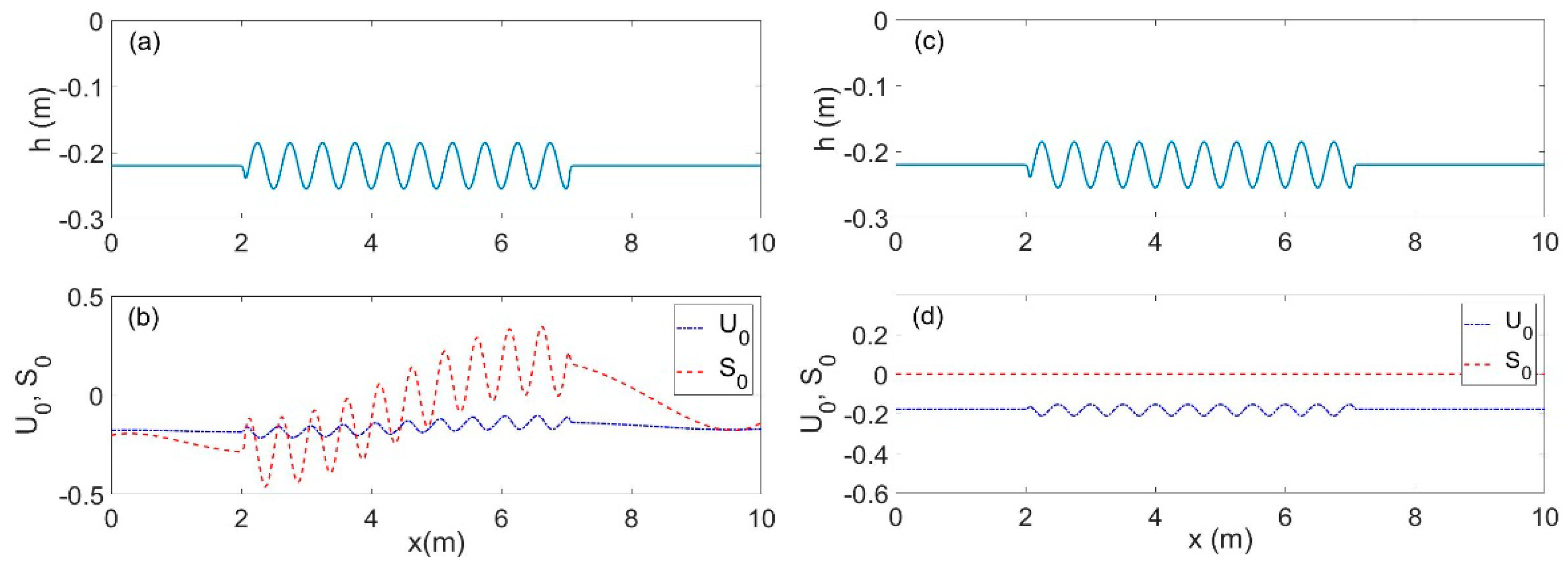
Next, we consider the reflection of waves in the same environment (
Figure 5a) with addition of an opposing current of mean speed 0.17 m/s. In this case, a distribution of the shear S(x) in the domain is estimated based on the measured vertical current profiles (see
Figure 3). This distribution is presented in
Figure 5b. The shear
S(
x) is negative near the entrance of the wave and becomes oscillatory above the ripple bed while its mean value increases, and eventually becomes positive near the downwave end of the sinusoidal bathymetry.
Based on the above data concerning
S(
x), the horizontal distribution of the surface current speed in the domain is calculated assuming conservation of the current mass flow as follows:
The comparison of the calculated reflection coefficient, based on wave potential (
) and the free surface elevation (
), is presented in
Figure 6a. We observe that the predicted modulus of the reflection coefficient near resonance (
= 0.42 and
= 0.33) is in some agreement with experimental data (
Rexp = 0.37), which is based on wave amplitude measurements upwave of the sinusoidal bottom; see also
Figure 2. However, the MMS overestimates the resonance frequency which is calculated at 1.16 Hz as compared with the experiment measurement 1.11 Hz. For comparison purposes, in
Figure 6b another calculation of the reflection coefficient is presented as also obtained by the present MMS by neglecting the shear. The latter assumption used in Equation (20) modifies slightly the surface current speed, as shown in
Figure 5d. We observe that the present MMS provides very similar predictions of the peak frequency of the reflection coefficient, indicating that this model is relatively insensitive to the shear contents of the opposing current field.
3.4. Investigation of Resonance Conditions and Discussion
The observed behavior of the MMS in the case of Bragg scattering of waves propagating over an undulating bottom in the presence of an opposing current, especially concerning the resonant frequency, can be explained by studying the properties of the second-order Equation (7) in the context of the parametric resonance of dynamical systems; see, e.g., [
24].
We consider again the simplified version of the present MMS, under the assumption of the small horizontal variation of parameters, as provided by Equation (11a), which is equivalently put in the form:
We observe that due to the depth variations, as described by Equation (2), in conjunction with variations of the current speed described by Equation (20), the dispersion relation Equation (5) will eventually lead to similar variations of the wavenumber,
, with
denoting the bottom wavenumber, and
the corresponding amplitude of the wavenumber due to bottom perturbation. Therefore, all coefficients of Equation (21), i.e., both
and
, are characterized by similar variations. Using the following representation of the solution
Equation (21) is put in the form
and the resonance is determined by the condition requiring the representative parameter
κ to become half of the bottom wavenumber
Kb:
On the other hand, it is known from standard theory [
25] that resonant reflection of surface water waves by sandbars in the presence of a current is manifested when
where
and
are obtained as the roots of Equations (5) and (13), respectively.
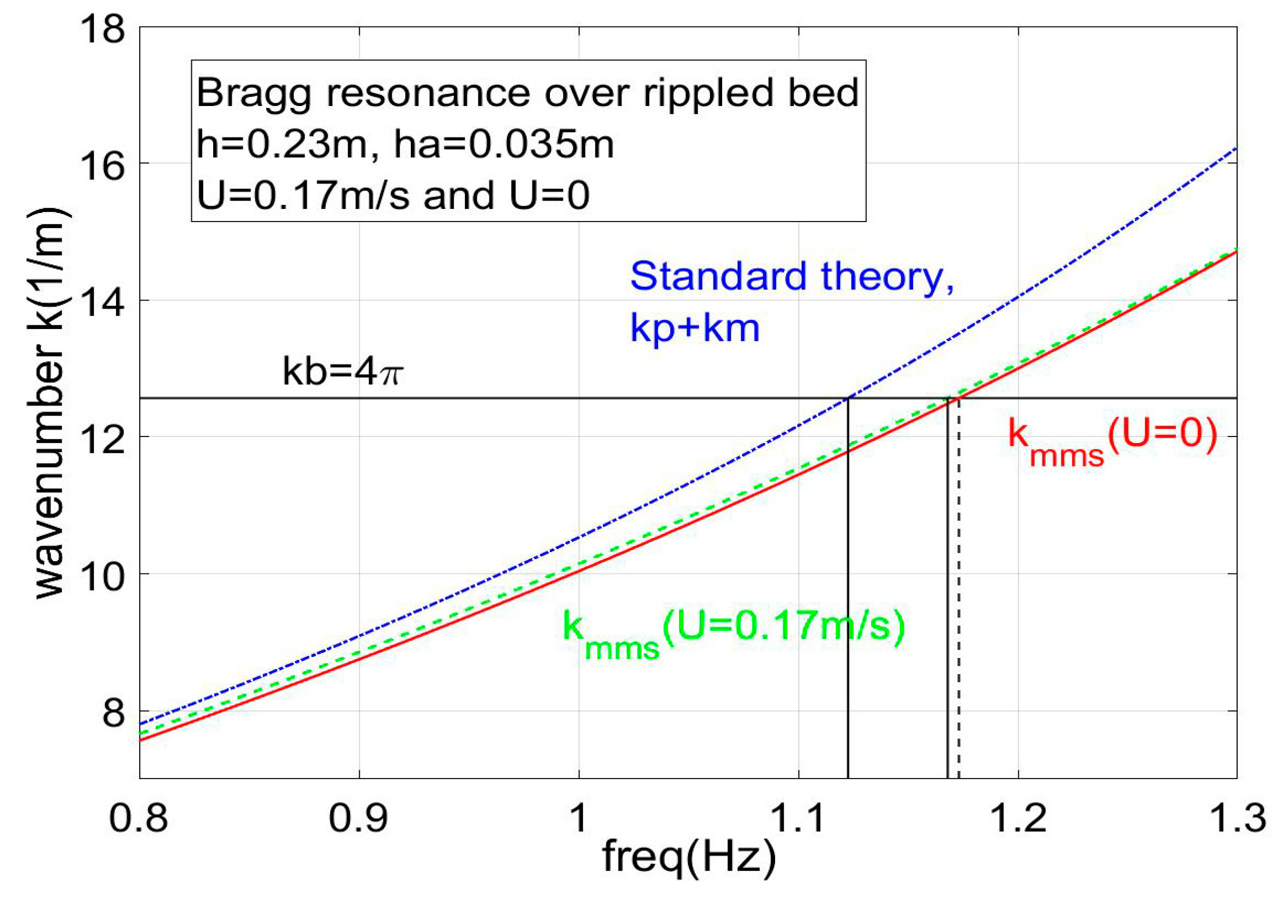
These dispersion relations are plotted together in
Figure 7, in a configuration corresponding to the present experimental conditions. The value of 2
, as obtained from the left-hand side of resonance condition, Equation (24a), appears as the solid line, denoted as “
kmms (
U = 0.17 m/s)”. Moreover, the value of
, corresponding to the left-hand side of the standard resonance condition Equation (24b), is also shown as the solid line denoted as “standard theory,
”. The dispersion equation obtained by the present MMS model, Equation (24a), in the absence of a current, is also plotted in this figure for reference, by using a dashed line denoted as “
kmms (
U = 0 m/s)”. In the specific case examined, the resonant conditions are manifested when the above dispersion curves intersect with the bottom wavenumber,
= 4π, which is shown by using a horizontal line.
It is shown that the present MMS provides a resonance frequency of 1.17 Hz without a current and this value is slightly reduced to 0.165 Hz when a current of mean speed 0.17 m/s is considered. On the contrary, the standard model, Equation (24b), results in a resonance frequency centered at 1.125 Hz, which is close to the experimental measurements; see also
Figure 6. It is also remarked that in the absence of a current, the above dispersion relation reduces to the same predictions concerning the resonant frequency.
It is concluded from the above analysis that the present one-equation MMS model, although it is found to be able to provide good predictions in inhomogeneous environments and flow conditions in the case of a smaller reflection where the direction of the wave propagation is well defined (as in the case of the waves over trapezoidal bar), it fails to provide accurate results in the case of multidirectional systems, as it happens to be near the resonance of scattered waves over bed ripples where both the forward- and back-propagating modes are strong.
4. Derivation of a Two-Equation Mild-Slope System
The purpose of the present work is first to explain why the MMS fails in the specific case characterized by strong backscattering and to propose a method to overcome this problem. A solution is offered by means of a coupled system describing the forward and backward wave propagation components. Such a mild-slope, two-equation system (CMS2) is developed in this section following the analysis presented by Belibassakis et al. [
18]. For this purpose, we use a representation of the wave system analyzed in forward- and back-propagating modes as follows:
where the vertical structure of the modes is given by
and the wavenumbers,
and
, are obtained from the dispersion relation of the forward and backward modes by Equations (5) and (13), respectively. For the derivation of the CMS2, we consider the variational principle presented by Belibassakis et al. [
18]:
where the term
4.1. The New CMS2
A coupled system of second-order equations with respect to the unknown modal amplitudes
is derived by using Expression (25) in the variational principle Equation (27), considering the relationship between the infinitesimal variations,
and
:
resulting in the following system of two equations
where
are given by Equations (9a)–(9c) and (10) using
and
, respectively. In Equation (30), the coefficients
are all functions of
x and are given by
where
.
4.2. Boundary Conditions for CMS2
Assuming weak shear at the ends of the domain
x = a corresponding to the wave incidence (in front of the wavemaker) and
x = b corresponding to the wave transmission zone (downwave end of the tank) and using the decomposition of the solution
the following boundary conditions are easily derived
which accurately model the required behavior of the wave components, respectively.
In the case of the CMS2, the reflection and transmission coefficients based on the wave potential are easily obtained as follows
and the corresponding coefficients are obtained by similar formulas applied to the free-surface elevation associated with each component
4.3. Application of CMS2 to Wave Reflection by the Sinusoidal Bottom and Opposing Current
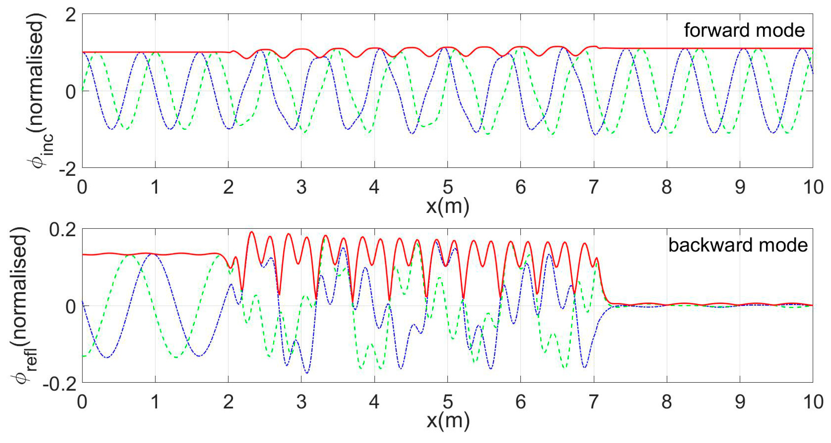
Results concerning the spatial evolution of waves in the considered environment with an opposing current of mean speed 0.17 m/s are presented in
Figure 8,
Figure 9,
Figure 10 and
Figure 11, for an incident wave frequency of 1.13 Hz near the expected resonance condition. Both cases of a shear current with
S(
x) distribution based on the measured data (
Figure 8 and
Figure 9) and of a current uniform in depth, involving no shear (
S = 0) (
Figure 10 and
Figure 11), are considered.
In these figures, solid lines indicate the real part, dashed lines the imaginary part and thick solid lines the spatial distribution of the modulus of both the forward and back-propagating modes, both concerning the wave potential and the calculated free surface elevation.
We observe in all cases that the back-propagating component, excited mainly over the rippled bed, becomes quite strong in the upwave subregion. Also, the consideration of a shear provides more complicated patterns of the physical quantities considered, especially over the sinusoidal bottom profile. Finally, comparisons between the calculated results by CMS2 and the experimental data concerning the modulus of the reflection coefficient are presented in
Figure 12. We observe that the present CMS2 is able to predict quite well the reflection properties including the resonance frequency, which is estimated to be 1.13 Hz, and the modulus of the reflection coefficient
= 0.41 and
= 0.31 in comparison to the experimental measurements, which are denoted by using open circles and dashed lines.
From the experimental data, the resonant frequency is observed to be 1.11 Hz and the reflection coefficient
= 0.36, respectively. On the other hand, it is observed that the CMS2, for the same case of waves and opposing current without shear, overestimates the resonance frequency and underestimates the value of the reflection coefficient, indicating that in the examined case the CMS2 is more sensitive to shear
S(
x) than the more simplified one-equation MMS model. This is due to the fact that the assumption of a vertically uniform current (
= 0) in Equation (20) results in a different distribution of surface current
, as presented comparatively in
Figure 5b,d, which has an effect on the coefficients of the present system CMS2 leading to the changes of reflection coefficient shown in
Figure 12b. As discussed in more detail in
Appendix A, the present model is based on the assumption that the shear S is a slowly varying function of the horizontal coordinate, and an additional source of error is possible due to vertical variations of S near the seabed associated with boundary layer viscous flow phenomena, which cannot be treated by the present model. Under the assumption that the above viscous effects do not significantly affect the global wave characteristics outside the seabed-boundary zone of small thickness compared to the water depth, it is shown that the present MMS model, being an averaged, in depth, one-equation model based on a specific assumption concerning the local vertical structure of the wave field of the form
, where
is an estimation of the forward propagating wavenumber, does not adequately predict strong reflection due to Bragg scattering.
The reason is that a second wave component is generated characterized by a different wavenumber, and the vertical structure of the wave field outside the viscous bottom boundary layer zone is not well represented by the above form, unless the two wavenumbers associated with the forward and backward modes are equal, which is the case for waves propagating over the rippled bed without a current. The problem is resolved by a system consisting of two interacting modes (CMS2) which behaves more efficiently.


