Latent Heat Flux Trend and Its Seasonal Dependence over the East China Sea Kuroshio Region

Abstract

Investigating latent heat flux (LHF) variations in the western boundary current region is crucial for understanding air–sea interactions. In this study, we examine the LHF trend in the East China Sea Kuroshio Region (ECSKR) from 1959 to 2021 using atmospheric and oceanic reanalysis datasets and find that the LHF has a significant strengthening trend. This strengthening can be attributed to sea surface warming resulting from the advection of sea surface temperatures. More importantly, the LHF trend has an apparent seasonal dependence: the most substantial increasing trend in LHF is observed in spring, while the trends are weak in other seasons. Further analysis illustrates that the anomaly of air–sea humidity difference plays a pivotal role in controlling the seasonal variations in LHF trends. Specifically, as a result of the different responses of the East Asian Trough to global warming across different seasons, during spring, the East Asian Trough significantly deepens, resulting in northerly winds that facilitate the intrusion of dry and cold air into the ECSKR region. This intensifies the humidity difference between the sea and air, promoting the release of oceanic latent heat. These findings can contribute to a better understanding of the surface heat budget balance within western boundary currents.

1. Introduction

The Kuroshio, the strong western boundary current in the North Pacific, originates from the bifurcation of the Northern Equatorial Current along the coast of the Philippines and flows northward through the Luzon Strait, enters the East China Sea (ECS) through the East Taiwan Strait, and exits the ECS through the Tokara Strait south of Kyushu Island [1]. It transports warm and salty water from the tropics to mid-latitudes, releasing significant heat into the atmosphere, particularly during winter, as cold and dry continental air is advected over the intense sea surface temperature (SST) gradient to waters that can be warmer than the air by 15° or more, leading to heat fluxes on the order of 1000 W/m² in the Kuroshio region [2,3]. This heat flux, known as turbulent heat flux (THF), which includes latent heat flux (LHF) and sensible heat flux (SHF), drives diabatic heating in the lower atmosphere and leads to long-term and synoptic-scale variations in atmospheric circulation [4,5,6]. Generally, LHF is significantly greater in magnitude (~2–3 times) than SHF over the Western Boundary Currents (WBCs) [7]. Furthermore, the THF (or LHF) between the atmosphere and WBCs is the most remarkable in the world’s oceans. These fluxes play an important role in global meridional heat transport and the transport of pollutants through air–sea exchange, exerting a significant influence on weather, climate, and the environment [8,9,10].

Over the past two decades, there has been a relative scarcity of attention towards the LHF over the Kuroshio mainstream compared to the Kuroshio Extension. However, it has come to light that the LHF over the Kuroshio in the ECS can have a notable influence on the prevailing atmospheric and oceanic conditions [11,12,13,14,15]. Bai et al. reported that variations in sea surface heat flux associated with the SST front result in anomalous vertical structures in the air–sea boundary layer [16]. This, in turn, strengthens local circulation and moisture conditions, thereby affecting precipitation in the middle and lower reaches of the Yangtze River and Southern China [17].

Currently, many studies have analyzed the LHF characteristics and roles in air–sea interactions across synoptic to interannual time scales [18,19,20,21], although they have not only focused on the Kuroshio region. Only several studies have investigated the long-term variations on ocean surface LHF, and they found that, on a global scale, positive linear trends in LHF are most significant over the tropical Indian and western Pacific warm pools as well as the boundary current regions [7,22,23]. In addition, some studies have revealed the relationship between SST and sea surface heat flux on long-term time scales over WBCs. For example, the warming SST is the primary driver for the enhanced LHF positive trend in the extended Brazil current region [23]. Li et al. found that SST is the main driving factor for the increase in LHF, while wind speed plays a secondary role in the long-term variations of LHF over the tropical and subtropical Pacific Ocean [24]. They also indicated that the consistent changes in LHF, temperature, and wind speed could be attributed to global warming [24].

In recent years, under the background of global warming, significant warming has been observed over the East China Sea Kuroshio Region (ECSKR) and the coastal area, with warming rates notably higher than the global average [25,26,27,28,29,30,31]. The sustained warming of SST can affect the LHF release over the Kuroshio current. As a key factor influencing climate and weather changes in the Northwest Pacific, understanding the sea surface LHF variations and trends over the Kuroshio region in the context of global warming is of great importance. In light of this, two fundamental questions arise: does the increase in SST promote the LHF release over the ECSKR? Considering the inherent seasonality of LHF, is there a seasonal dependence in its long-term variability?

In this study, we utilize long-term reanalysis datasets to determine the trends and seasonal differences in LHF in the ECSKR. Through estimating related variables using the bulk aerodynamic formula, we explore the primary factors driving the long-term trend and the seasonal dependence of LHF in the Kuroshio region and the associated physical mechanisms. The remaining sections of this paper are organized as follows: Section 2 describes the data and methods employed in this study. Section 3 investigates the climatological mean state of the LHF over ECSKR. The long-term trend of LHF over the ECSKR and its seasonal dependence are investigated in Section 4. Section 5 presents a discussion, and Section 6 provides a conclusion.

2. Data and Methods

2.1. The Fifth-Generation Global Atmospheric Reanalysis (ERA5)

The ERA5 reanalysis dataset was released by the European Centre for Medium-Range Weather Forecasts (ECMWF) [32], which offers hourly and monthly data on various atmospheric, land surface, and sea state parameters, along with estimations of uncertainty. This comprehensive dataset integrates model data with global observations, ensuring consistency through the application of physical principles. This dataset covers the entire globe with an original spatial resolution of 0.28° (approximately 31 km) and provides hourly outputs from 1950 to the present (with a 5-day delay). These characteristics make ERA5 suitable for a wide range of applications, including climate monitoring, research, education, policy-making, commercial purposes, as well as sectors like renewable energy and agriculture [33]. ERA5 data can be accessed in the Climate Data Store, presented on regular latitude-longitude grids at a resolution of 0.25° × 0.25°, encompassing atmospheric parameters across 37 pressure levels from 1940 to the present day. In this study, we analyze monthly gridded ocean surface LHF data and related surface oceanic and meteorological fields, such as surface air temperature, 2 m air dewpoint temperature, 10 m wind speed, and SST for 1959–2021.

2.2. Ocean Reanalysis System 5 Reanalysis (ORAS5)

In this study, we also use ECMWF ORAS5 monthly data to calculate mixed layer heat advection. The ORAS5 data employ ocean models utilizing Mercator coordinate grids south of the Arctic, which have been adjusted at high latitudes to prevent meridian convergence [34]. This dataset includes 75 vertical levels, with finer 1 m intervals near the surface, and 24 of these levels are within the upper 100 m. The approximately 0.25° × 0.25° (around 25 km in the tropics and 9 km in the Arctic) monthly gridded meridional and zonal velocity, potential temperature, and mixed layer depth (the depth of the ocean where the average sea water density exceeds the near surface density plus 0.03 kg/m³) are used. The time period of the ORAS5 data used is the same as the ERA5 data.

2.3. Goddard Institute for Space Studies Surface Temperature Analysis (GISTEMP) v4

GISTEMP [35] is a widely utilized product that leverages in situ surface measurements over land, compiled from publicly accessible surface air temperature data collected by approximately 6300 meteorological stations globally. Additionally, it incorporates an analysis of ship- and buoy-based SST [36], as well as data from Antarctic weather stations. We use global mean monthly SST data to examine the potential impacts of global warming.

2.4. The Coupled Ocean–Atmosphere Response Experiment (COARE) 3.5 Bulk Flux Algorithm

To estimate the contributions of variables to LHF changes, we apply the COARE 3.5 bulk flux algorithm [37,38] derived from the Monin–Obukhov similarity theory [39],

$$\mathrm{L}\mathrm{H}\mathrm{F}={\rho }_a{L}_e{C}_{e}U\Delta q={\rho }_a{L}_e{C}_{e}U\left(q_s-q_a\right),$$

(1)

where ${\rho }_a$ is the density of air, $L_e$ is the latent heat of vaporization, $C_e$ is the turbulent transfer coefficient of latent heat, $U$ is the scalar surface wind speed (typically at 10 m), $\Delta q$ is the air–sea-specific humidity difference, $q_s$ is the surface saturation specific humidity, and $q_a$ is the surface air specific humidity (usually at 2 m). Note that $q_s$ is computed from the saturation humidity $q_{sat}$ for pure water at skin SST $T_s$ [40]:

$$q_s=0.98q_{sat}\left(T_s\right).$$

(2)

In this study, ${\rho }_a$, $L_e$, $C_e$, $q_s$, and $q_a$ are calculated by the COARE toolkit using required data from ERA5. The COARE toolkit is provided by the National Oceanic and Atmospheric Administration.

To quantitatively estimate which factor is dominant in determining change in LHF, we follow the approach of Alexander and Scott and Tanimoto et al. [18,41] to rewrite the bulk formula for LHF in terms of time mean quantities and anomalies, as follows:

$$\begin{array}{cc}{\mathrm{LHF}}^{\mathrm{’}}& =\mathrm{LHF}-\overline{\mathrm{LHF}}\hfill \\ & ={\rho }_a{L}_e{C}_e\left\{U^{’}\left({\overline{q}}_s-{\overline{q}}_a\right)+\overline{U}{q}_s^{’}-\overline{U}{q}_a^{’}+\left[U^{’}\left(q_s^{’}-q_a^{’}\right)-\overline{U^{’}\left(q_s^{’}-q_a^{’}\right)}\right]\right\},\hfill \end{array}$$

(3)

where primes denote deviations from the mean and overbars are the time mean. In practice, we use climatological monthly means for overbar terms and deviations from climatological means for deviation terms. The items within square brackets are very small (see Figure S1 in Supporting Information) and have been neglected.

In practice, before evaluating the contribution of bulk variables to the trend of LHF using the COARE algorithm, we first need to confirm whether the estimated LHF by the COARE is consistent with that from ERA5 data. Figures S2 and S3 in the supporting information show that the LHF calculated by the COARE algorithm is generally consistent with ERA5, although slightly underestimated, which does not affect our trend contribution analysis.

2.5. The Student’s t-Test

In this paper, the linear trends (regression coefficients) are calculated by the least squares method. We use the Student’s t-test to test the significance of a linear trend. The null hypothesis H0 of the Student’s t-test is that there is no significant trend.

For time-varying atmospheric or oceanic data $y$, we use the least squares method to achieve its linear trend $a$. The residuals of regression, $e$, are defined as $e=\left(ax+b\right)-y$, where $x$ is time and $b$ is intercept. The standard error of the regression coefficient is

$$SE\left(a\right)=\sqrt{\frac{{\sum }_{i=1}^n{e}^2}{(n-2){\sum }_{i=1}^n{(x_i-\overline{x})}^2}},$$

(4)

where $n$ is the amount of data. Then the t-value is

$$t=\frac{a}{SE\left(a\right)}.$$

(5)

Here, we use the t-distribution with degrees of freedom $n-2$ to calculate the p-value. If the p-value is less than 0.025 (95% significance level), then we can reject the null hypothesis, indicating that there is a linear trend between the time $x$ and the dependent variable $y$.

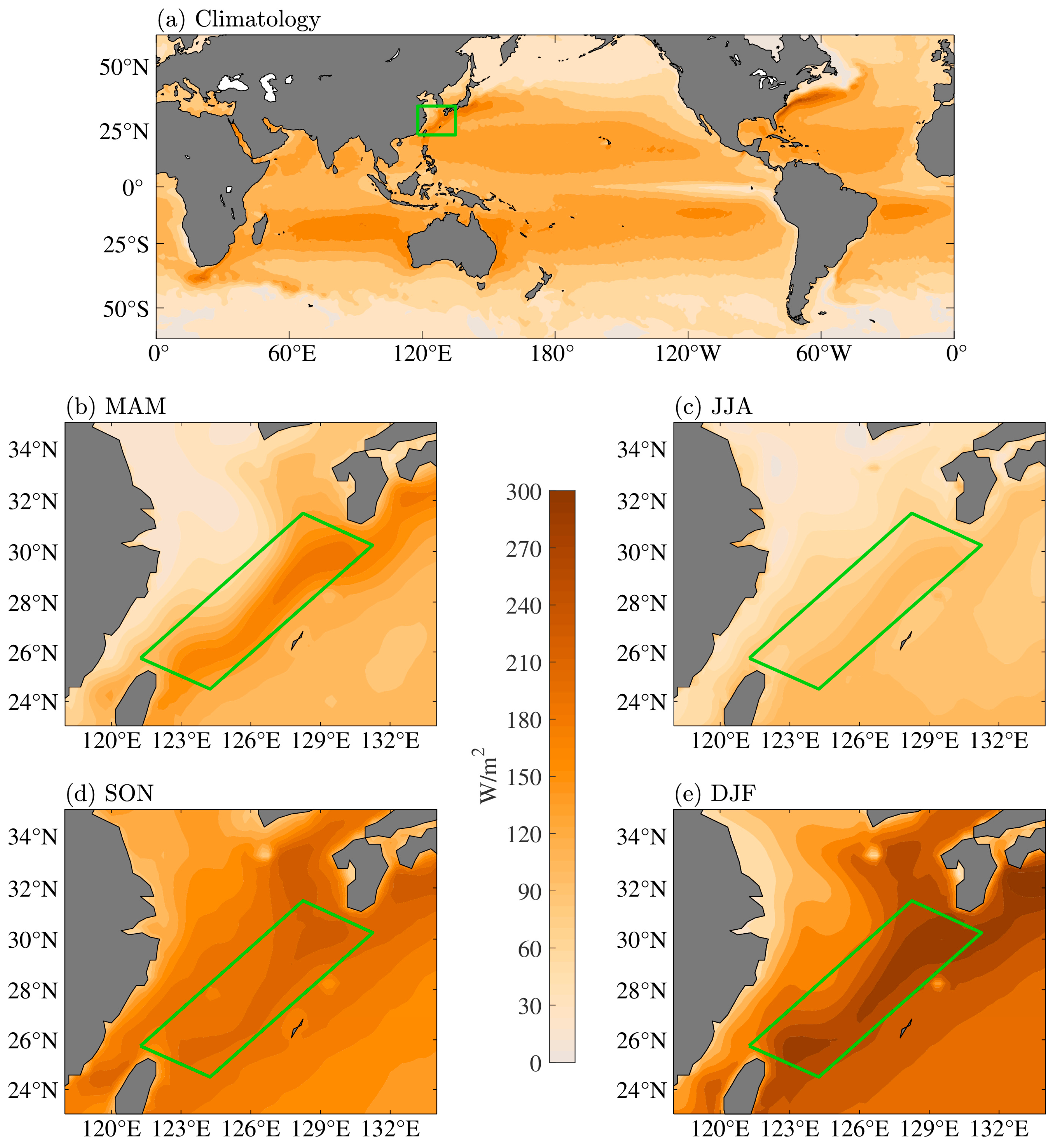
3. LHF Climatological Mean State in the ECSKR

Figure 1a shows the climatology features of LHF over the global ocean between 60° S and 60° N. It is evident that the Kuroshio and Gulf Stream regions are the main areas for LHF release in the Northern Hemisphere. This article mainly focuses on the Kuroshio region in the ECS (the green box in Figure 1a). Figure 1b–e show seasonal climatology for the four seasons in the ECS region. The spatial distribution is inhomogeneous, and the large values are along the Kuroshio axis (green box in Figure 1b–e), implying that the LHF has a strong relationship with the Kuroshio, which is in good agreement with previous studies [42,43,44].

In terms of seasonal variations, the LHF exhibits the highest magnitude during winter, followed by fall and spring, and the lowest one in summer. The maximum values of LHF are concentrated along the axis of the Kuroshio in each season. This infers the ECS’s significant role as a crucial heat dissipation region in the North Pacific, with the Kuroshio playing a vital role. During winter, the ECSKR exhibits the highest magnitude of latent heat release, reaching an average of 300 W/m². This can be attributed to the intense northerly winds and substantial disparities in air–sea humidity differences. In summer, due to the southerly wind and the weak humidity difference, the LHF in the ECSKR sharply decreases, with the maximum value along the Kuroshio current axis, where the LHF is only ~120 W/m².

Overall, the LHF demonstrates a distinct seasonal pattern in the ECSKR. Therefore, in order to investigate trends in the LHF within the study area, it is essential to evaluate the trend for each season separately. Furthermore, Figure 1 highlights the significant influence of ocean currents on LHF, necessitating a careful analysis of trends while considering the impact of these currents on the heat flux. It is worth noting that previous analyses of heat fluxes in the ECSKR predominantly relied on annual averages, without distinguishing between different season periods.

4. LHF Trend and Its Seasonal Dependence over the ECSKR

4.1. The Increasing Trend of LHF and Its Seasonal Dependence

Figure 2 shows the surface LHF linear trend for different seasons in the ECS, which exhibits a significant increasing trend of LHF in both the ESCKR and the western part of the ECS. More interestingly, the LHF trend demonstrates an obvious seasonal dependence, with the strongest growth in spring and the weakest one in summer. In addition to the student’s t-test, the Mann–Kendall test [45,46] is also widely used as a reliable method for trend test. In fact, we also employed the Mann–Kendall trend test to examine the trend of LHF (see Text S1) and found that the results of the Mann–Kendall trend test are generally consistent with the Student’s t-test, comparing Figures S4 and S5 in the supporting information with Figure 2.

To validate the robustness of this result, the trend analysis has also been performed based on the 20CRv3 and OAFlux datasets (detailed information about the datasets can be found in Texts S2 and S3 of Supporting Information). Despite the different time ranges covered by these two datasets compared to ERA5, long-term LHF trends and their seasonal variations, as depicted in Figures S6 and S7, are consistent with Figure 2. In particular, for ERA5, the ECSKR area-mean trend of LHF is 2.59 ± 0.32 W/m² per decade in spring during 1959–2021, followed by 1.54 ± 0.34 W/m² per decade in winter. The weakest trend emerges in the summer with 0.48 ± 0.17 W/m² per decade.

4.2. Dominant Factors Causing the Positive Trend of LHF

To achieve a better understanding of the LHF trend, we apply the COARE 3.5 algorithm to quantitively identify which bulk variables (Equations (1)–(3)) determine this trend. Figure 3 illustrates the spatial distribution of linear trend of each term in Equation (3), which can quantify the contributions from $U^{’}$, $q_s^{’}$, $q_a^{’}$, and $\Delta q$ to the total surface LHF trend, respectively. It is evident that $U^{’}$ has a relatively smaller impact (Figure 3a–d), compared to $q_s^{’}-q_a^{’}$ (Figure 3m–p). In addition, air–sea-specific humidity differences ($\Delta q$) in Figure 3m–p exhibit a remarkably similar spatial structure and magnitude to Figure 2a–d. This suggests that the long-term trend of LHF is predominantly influenced by fluctuations in local air–sea humidity differences rather than local wind speed. Furthermore, $q_s^{’}$ in Figure 3e–h show a significant positive trend, indicating its positive contribution to local LHF. The changes in the near sea surface air humidity $q_a^{’}$ in Figure 3i–l display a negative trend and play a decreasing role in LHF. More quantitatively, we calculate the area average value of each term in Equation (3) in the ECSKR, as shown in Figure 4. Indeed, the sea surface air humidity change $q_s^{’}$ presents a large positive value, while $q_a^{’}$ has a negative value. This reveals that $q_s^{’}$ ($q_a^{’}$) promotes (suppresses) the release of latent heat.

As is well known, although $q_s$ is calculated by Equation (2) using the skin SST, it is closely related to SST. As such, we show the variations of SST together with $q_s$ over the ECSKR in Figure 5. The figure indicates a significant interdecadal variability. The decade-to-decade fluctuations in SST and $q_s$ demonstrate a remarkable correlation. To validate this relationship, linear trends (

Table 1. Trend of the surface LHF and related surface bulk variables averaged over the ECSKR ^a.

Trend Slope per DECADE	Spring	Summer	Fall	Winter
$\mathrm{SST} (°C$)	0.12 ± 0.01	0.12 ± 0.01	0.12 ± 0.01	0.15 ± 0.01
$\mathrm{SAT} (°C$)	0.11 ± 0.02	0.13 ± 0.01	0.15 ± 0.01	0.20 ± 0.02
$q_s$ (g/kg)	0.11 ± 0.01	0.16 ± 0.01	0.15 ± 0.01	0.13 ± 0.01
$q_a$ (g/kg)	0.02 ± 0.01 *	0.13 ± 0.01	0.11 ± 0.02	0.10 ± 0.01
$\Delta q$ (g/kg)	0.10 ± 0.01	0.03 ± 0.01	0.04 ± 0.01	0.03 ± 0.01
LHF (W/m2)	2.59 ± 0.32	0.48 ± 0.17	1.13 ± 0.22	1.54 ± 0.34

^a The symbol “*” indicates the trend that does not exceed the 95% confidence level. The trends without “*” denote that they pass the 95% significance tests.

) and correlation coefficients (shown in Figure 5) are given for the time series of LHF and the bulk variables. For all four seasons, SST exhibits a strong positive correlation with $q_s$, with coefficients of 0.999 (spring), 0.999 (summer), 1.000 (fall), and 1.000 (winter), respectively. We also examined the spatial correlation between LHF and SST. The results, as shown in Figure S8 in the supporting information, demonstrate similar spatial patterns, which is consistent with Figure 6. This indicates a robust relationship between SST and $q_s$. Thus, the local enhancement of SST is the main driving factor for the growth of LHF in this area during 1959–2021.

To further demonstrate the rise in SST, we plot the spatial structure of the SST trend in Figure 6a–d. The SST has a significant increase in winter and spring in the ECSKR and nearshore area, while the increase is relatively weak in summer and autumn, which appears to be consistent with the trend of LHF (Figure 2). This again confirms the dominant contribution of SST to the LHF trend. In fact, the significant increase in SST in the ECSKR has been acknowledged and investigated by some previous studies, in which oceanic lateral heat advection was found to play a primary role [30,47]. Furthermore, in order to clarify which advection process ($-\left(\overline{\mathrm{U}}·\nabla \mathrm{T}\right)$ or $-(\mathrm{U}·\nabla \overline{\mathrm{T}})$) is more important, we indicate their time average spatial patterns in Figure 6, where $-\left(\overline{\mathrm{U}}·\nabla \mathrm{T}\right)$ denotes the SST advection by climatological surface flow velocity, $-(\mathrm{U}·\nabla \overline{\mathrm{T}})$ represents the advection of climatological SST by surface flow velocity. The figure shows that $-\left(\overline{\mathrm{U}}·\nabla \mathrm{T}\right)$ has a more pronounced effect in spring and winter compared to summer and autumn, whereas $-(\mathrm{U}·\nabla \overline{\mathrm{T}})$ exhibits opposite behavior. Meanwhile, the spatial structures of the SST trend in spring and winter (summer and autumn) are similar to those of $-\left(\overline{\mathrm{U}}·\nabla \mathrm{T}\right)$ ($-(\mathrm{U}·\nabla \overline{\mathrm{T}})$) in the ECSKR. This reflects that the SST trend in the ECSKR during spring and winter is determined by SST advection by the climatological flow velocity, while the trend in summer and autumn is caused by the climatological SST advection by flow velocity.

4.3. Possible Mechanism for Seasonal Dependence of the LHF Trend

Another crucial aspect of the LHF trends over the ECSKR is their seasonal variations. Figure 3 and Figure 4 clearly illustrate that the highest LHF trend in spring is due to the low negative contribution of $q_a^{’}$ compared to the other three seasons, despite the positive contribution from $q_s^{’}$ being relatively lower than that of the other seasons. In this situation, the variations in sea surface air humidity $q_a^{’}$ contribute to those ($q_s^{’}-q_a^{’}$) of the air–sea-specific humidity difference (Figure 4), which yields the seasonal difference.

The results regarding the impact of atmospheric humidity advection on the anomaly of air–sea humidity difference in the ECSKR, as determined through regression analysis, are presented in Figure 7. In spring, a pressure decreasing trend occurs over Japan, resulting in stronger northerly winds (as seen in vectors), which transport dry and cold air from the north into the ECSKR, thereby enhancing the air–sea humidity difference. This indicates that the deepening East Asian trough (EAT) strengthens the northerly winds, resulting in more cold air from the mainland moving southward to affect LHF over ECSKR. In summer, the impact of this pressure decreasing is primarily felt in the northeastern region of Japan and greatly weakened in fall. In winter, it appears in the center of the North Pacific and has a little impact on the East China Sea. The regression findings reveal a significant influence of atmospheric humidity advection, with the most pronounced effect in spring. This is the reason for the strongest increase in the LHF trend in spring over the ECSKR.

The LHF, geopotential height field, and wind field all exhibit consistent seasonal variations, with the EAT playing a crucial role in this process. This may indicate the presence of a common cause leading to their synchronized changes. Recent studies have shown that global warming plays an important role in the evolution of the EAT, which will affect the atmospheric circulation throughout East Asia [48,49]. We regress 850 hpa moisture advection, 850 hpa wind speed, and 500 hpa geopotential height against the GISTEMP global average surface temperature (Figure 8). The results show that the deepening effect of global warming on spring EAT corresponds well to the results of Figure 7. This demonstrates that the seasonal dependence of the LHF trend in the ECSKR region may be the result of different seasonal responses of EAT to global warming. These findings suggest a robust correlation between the trends in LHF over the ECSKR and the East Asian atmospheric circulation response to global warming, revealing the important role of atmospheric forcing in the long-term variations of air–sea interactions.

5. Discussions

5.1. Significance of the Study

Our study contributes to a better understanding of the air–sea interaction processes in the Kuroshio region and their response to global warming. The significance of our findings can be summarized as follows:

Identification of dominant drivers: We identify SST as the primary driving factor for the increasing trend of LHF. This highlights the crucial role of oceanic processes, such as the Kuroshio current, in modulating air–sea heat exchange.

Seasonal dependence of the LHF trend: The observed seasonal dependence of the LHF trend underscores the importance of considering seasonal variations in future studies. Our findings emphasize the need for a seasonal approach when analyzing long-term trends in air–sea interaction processes.

Implications for climate research: Understanding the mechanisms driving the observed trends in LHF is essential for accurately assessing the impacts of global warming on regional climate and weather patterns.

5.2. Future Research Directions

While our study provides valuable insights into the long-term trends and seasonal variations of LHF over the ECSKR, several avenues for future research exist:

Reduce the uncertainty of data: Although the three sets of data used in this paper show a consistent trend and seasonal dependence, there are still large differences in their magnitude and detailed patterns. Reducing the error and uncertainty of data is a direction of work.

Modeling studies: Numerical modeling studies can help simulate the complex interactions between oceanic currents, atmospheric circulation, and heat exchange processes over the ECSKR, providing additional insights into the observed trends.

Regional climate projections: Understanding how the observed trends in LHF over the ECSKR may evolve in the future under different climate change scenarios is crucial for regional climate projections and adaptation strategies, especially for neighboring countries.

In conclusion, our study enhances our understanding of the air–sea interaction processes over the Kuroshio region and provides valuable insights into the response of these processes to global warming. Our findings underscore the importance of considering seasonal variations when analyzing long-term trends in air–sea heat exchange and have implications for regional climate research and projections.

6. Conclusions

We examined the LHF trends in the ECS region from 1959 to 2021, mainly using the ERA5 reanalysis dataset from ECMWF. It was demonstrated that there exists a robust, increasing trend in LHF. This trend is primarily observed in the Kuroshio and western parts of the ECS, exhibiting uneven patterns across the entire ECS. Analysis of bulk variables indicates that this growth in LHF is correlated with the elevated sea surface humidity associated with SST. The significant increase in SST might be associated with the enhanced ocean heat transfer by the Kuroshio current in the ECS. A rising SST trend initiates heightened specific humidity in the air–sea interface and greater disparities in temperature, resulting in stronger LHF release.

Interestingly, the increasing trend of LHF displays seasonal variability, with the strongest growth in spring and weak growth in summer and fall. The trend contributions of bulk variables show that the anomaly of air–sea humidity difference plays a vital role in this peculiar phenomenon. Regression results indicate that deepening of the EAT causes the strongest northerly winds, carrying cold and dry air, which contributes to the anomaly of air–sea humidity difference over the ECSKR and subsequently enhances the LHF in spring. In other seasons, the impact of EAT on the ECSKR is not significant. Further, we find that the forcing of global warming may lead to this EAT change in spring, which determines the unique seasonal dependence of the LHF trend.

References

1. Ichikawa, H.; Beardsley, R.C. The Current System in the Yellow and East China Seas. J. Oceanogr. 2002, 58, 77–92. [Google Scholar] [CrossRef]
2. Kelly, K.A.; Small, R.J.; Samelson, R.M.; Qiu, B.; Joyce, T.M.; Kwon, Y.-O.; Cronin, M.F. Western Boundary Currents and Frontal Air–Sea Interaction: Gulf Stream and Kuroshio Extension. J. Clim. 2010, 23, 5644–5667. [Google Scholar] [CrossRef]
3. Jensen, T.G.; Campbell, T.J.; Allard, R.A.; Small, R.J.; Smith, T.A. Turbulent Heat Fluxes during an Intense Cold-Air Outbreak over the Kuroshio Extension Region: Results from a High-Resolution Coupled Atmosphere–Ocean Model. Ocean Dyn. 2011, 61, 657–674. [Google Scholar] [CrossRef]
4. Joyce, T.M.; Kwon, Y.-O.; Yu, L. On the Relationship between Synoptic Wintertime Atmospheric Variability and Path Shifts in the Gulf Stream and the Kuroshio Extension. J. Clim. 2009, 22, 3177–3192. [Google Scholar] [CrossRef]
5. Kwon, Y.-O.; Alexander, M.A.; Bond, N.A.; Frankignoul, C.; Nakamura, H.; Qiu, B.; Thompson, L.A. Role of the Gulf Stream and Kuroshio–Oyashio Systems in Large-Scale Atmosphere–Ocean Interaction: A Review. J. Clim. 2010, 23, 3249–3281. [Google Scholar] [CrossRef]
6. Nakamura, H.; Nishina, A.; Minobe, S. Response of Storm Tracks to Bimodal Kuroshio Path States South of Japan. J. Clim. 2012, 25, 7772–7779. [Google Scholar] [CrossRef]
7. Yu, L.; Weller, R.A. Objectively Analyzed Air–Sea Heat Fluxes for the Global Ice-Free Oceans (1981–2005). Bull. Am. Meteorol. Soc. 2007, 88, 527–540. [Google Scholar] [CrossRef]
8. Cronin, M.F.; Gentemann, C.L.; Edson, J.; Ueki, I.; Bourassa, M.; Brown, S.; Clayson, C.A.; Fairall, C.W.; Farrar, J.T.; Gille, S.T.; et al. Air-Sea Fluxes with a Focus on Heat and Momentum. Front. Mar. Sci. 2019, 6, 450. [Google Scholar] [CrossRef]
9. Yu, L. Global Air–Sea Fluxes of Heat, Fresh Water, and Momentum: Energy Budget Closure and Unanswered Questions. Annu. Rev. Mar. Sci. 2019, 11, 227–248. [Google Scholar] [CrossRef]
10. Yang, M.; Guo, X.; Ishizu, M.; Miyazawa, Y. The Kuroshio Regulates the Air–Sea Exchange of PCBs in the Northwestern Pacific Ocean. Environ. Sci. Technol. 2022, 56, 12307–12314. [Google Scholar] [CrossRef]
11. Xu, H.; Xu, M.; Xie, S.-P.; Wang, Y. Deep Atmospheric Response to the Spring Kuroshio over the East China Sea. J. Clim. 2011, 24, 4959–4972. [Google Scholar] [CrossRef]
12. Sasaki, Y.N.; Minobe, S.; Asai, T.; Inatsu, M. Influence of the Kuroshio in the East China Sea on the Early Summer (Baiu) Rain. J. Clim. 2012, 25, 6627–6645. [Google Scholar] [CrossRef]
13. Kunoki, S.; Manda, A.; Kodama, Y.-M.; Iizuka, S.; Sato, K.; Fathrio, I.; Mitsui, T.; Seko, H.; Moteki, Q.; Minobe, S.; et al. Oceanic Influence on the Baiu Frontal Zone in the East China Sea. J. Geophys. Res. Atmos. 2015, 120, 449–463. [Google Scholar] [CrossRef]
14. Liu, J.-W.; Xie, S.-P.; Yang, S.; Zhang, S.-P. Low-Cloud Transitions across the Kuroshio Front in the East China Sea. J. Clim. 2016, 29, 4429–4443. [Google Scholar] [CrossRef]
15. Xu, M.; Xu, H.; Ren, H. Influence of Kuroshio SST Front in the East China Sea on the Climatological Evolution of Meiyu Rainband. Clim. Dyn. 2018, 50, 1243–1266. [Google Scholar] [CrossRef]
16. Bai, H.; Hu, H.; Ren, X.; Yang, X.-Q.; Zhang, Y.; Mao, K.; Zhao, Y. The Impacts of East China Sea Kuroshio Front on Winter Heavy Precipitation Events in Southern China. J. Geophys. Res. Atmos. 2023, 128, e2022JD037341. [Google Scholar] [CrossRef]
17. Bai, H.; Hu, H.; Perrie, W.; Zhang, N. On the Characteristics and Climate Effects of HV-WCP Events over the Kuroshio SST Front during Wintertime. Clim. Dyn. 2020, 55, 2123–2148. [Google Scholar] [CrossRef]
18. Alexander, M.A.; Scott, J.D. Surface Flux Variability over the North Pacific and North Atlantic Oceans. J. Clim. 1997, 10, 2963–2978. [Google Scholar] [CrossRef]
19. Araligidad, N.M.; Maloney, E.D. Wind-Driven Latent Heat Flux and the Intraseasonal Oscillation. Geophys. Res. Lett. 2008, 35, L04815. [Google Scholar] [CrossRef]
20. Foltz, G.R.; Grodsky, S.A.; Carton, J.A.; McPhaden, M.J. Seasonal Mixed Layer Heat Budget of the Tropical Atlantic Ocean. J. Geophys. Res. Oceans 2003, 108, 3146. [Google Scholar] [CrossRef]
21. Behera, S.K.; Salvekar, P.S.; Yamagata, T. Simulation of Interannual SST Variability in the Tropical Indian Ocean. J. Clim. 2000, 13, 3487–3499. [Google Scholar] [CrossRef]
22. Liu, J.; Curry, J.A. Variability of the Tropical and Subtropical Ocean Surface Latent Heat Flux during 1989–2000. Geophys. Res. Lett. 2006, 33, L05706. [Google Scholar] [CrossRef]
23. Leyba, I.M.; Solman, S.A.; Saraceno, M. Trends in Sea Surface Temperature and Air–Sea Heat Fluxes over the South Atlantic Ocean. Clim. Dyn. 2019, 53, 4141–4153. [Google Scholar] [CrossRef]
24. Li, G.; Ren, B.; Yang, C.; Zheng, J. Revisiting the Trend of the Tropical and Subtropical Pacific Surface Latent Heat Flux during 1977–2006. J. Geophys. Res. Atmos. 2011, 116, D10115. [Google Scholar] [CrossRef]
25. Belkin, I.M. Rapid Warming of Large Marine Ecosystems. Prog. Oceanogr. 2009, 81, 207–213. [Google Scholar] [CrossRef]
26. Tang, X.; Wang, F.; Chen, Y.; Li, M. Warming Trend in Northern East China Sea in Recent Four Decades. Chin. J. Oceanol. Limnol. 2009, 27, 185–191. [Google Scholar] [CrossRef]
27. Wu, L.; Cai, W.; Zhang, L.; Nakamura, H.; Timmermann, A.; Joyce, T.; McPhaden, M.J.; Alexander, M.; Qiu, B.; Visbeck, M.; et al. Enhanced Warming over the Global Subtropical Western Boundary Currents. Nat. Clim. Chang. 2012, 2, 161–166. [Google Scholar] [CrossRef]
28. Bao, B.; Ren, G. Climatological Characteristics and Long-Term Change of SST over the Marginal Seas of China. Cont. Shelf Res. 2014, 77, 96–106. [Google Scholar] [CrossRef]
29. Trenberth, K.; Jones, P.; Ambenje, P.; Bojariu, R.; Easterling, D.; Klein Tank, A.; Parker, D.; Rahimzadeh, F.; Renwick, J.; Rusticucci, M.; et al. Observations: Surface and Atmospheric Climate Change. In Climate Change 2007: The Physical Science Basis. Contribution of Working Group 1 to the 4th Assessment Report of the Intergovernmental Panel on Climate Change; Solomon, S., Qin, D., Manning, M., Chen, Z., Marquis, M., Averyt, K., Tignor, M., Miller, H., Eds.; Cambridge University Press: Cambridge, UK, 2007. [Google Scholar]
30. Cai, R.; Tan, H.; Kontoyiannis, H. Robust Surface Warming in Offshore China Seas and Its Relationship to the East Asian Monsoon Wind Field and Ocean Forcing on Interdecadal Time Scales. J. Clim. 2017, 30, 8987–9005. [Google Scholar] [CrossRef]
31. Toda, M.; Watanabe, M. Mechanisms of Enhanced Ocean Surface Warming in the Kuroshio Region for 1951–2010. Clim. Dyn. 2020, 54, 4129–4145. [Google Scholar] [CrossRef]
32. Hersbach, H.; Bell, B.; Berrisford, P.; Hirahara, S.; Horányi, A.; Muñoz-Sabater, J.; Nicolas, J.; Peubey, C.; Radu, R.; Schepers, D.; et al. The ERA5 Global Reanalysis. Q. J. R. Meteorol. Soc. 2020, 146, 1999–2049. [Google Scholar] [CrossRef]
33. Buontempo, C.; Hutjes, R.; Beavis, P.; Berckmans, J.; Cagnazzo, C.; Vamborg, F.; Thépaut, J.-N.; Bergeron, C.; Almond, S.; Amici, A.; et al. Fostering the Development of Climate Services through Copernicus Climate Change Service (C3S) for Agriculture Applications. Weather. Clim. Extrem. 2020, 27, 100226. [Google Scholar] [CrossRef]
34. Zuo, H.; Balmaseda, M.A.; Tietsche, S.; Mogensen, K.; Mayer, M. The ECMWF Operational Ensemble Reanalysis–Analysis System for Ocean and Sea Ice: A Description of the System and Assessment. Ocean Sci. 2019, 15, 779–808. [Google Scholar] [CrossRef]
35. Hansen, J.; Ruedy, R.; Sato, M.; Lo, K. Global Surface Temperature Change. Rev. Geophys. 2010, 48, RG4004. [Google Scholar] [CrossRef]
36. Huang, B.; Thorne, P.W.; Banzon, V.F.; Boyer, T.; Chepurin, G.; Lawrimore, J.H.; Menne, M.J.; Smith, T.M.; Vose, R.S.; Zhang, H.-M. Extended Reconstructed Sea Surface Temperature, Version 5 (ERSSTv5): Upgrades, Validations, and Intercomparisons. J. Clim. 2017, 30, 8179–8205. [Google Scholar] [CrossRef]
37. Fairall, C.W.; Bradley, E.F.; Rogers, D.P.; Edson, J.B.; Young, G.S. Bulk Parameterization of Air-Sea Fluxes for Tropical Ocean-Global Atmosphere Coupled-Ocean Atmosphere Response Experiment. J. Geophys. Res. Ocean. 1996, 101, 3747–3764. [Google Scholar] [CrossRef]
38. Fairall, C.W.; Bradley, E.F.; Hare, J.E.; Grachev, A.A.; Edson, J.B. Bulk Parameterization of Air–Sea Fluxes: Updates and Verification for the COARE Algorithm. J. Clim. 2003, 16, 571–591. [Google Scholar] [CrossRef]
39. Monin, A.S.; Obukhov, A.M. Basic Laws of Turbulent Mixing in the Surface Layer of the Atmosphere. Contrib. Geophys. Inst. Acad. Sci. USSR 1954, 151, e187. [Google Scholar]
40. Yu, L.; Jin, X.; Weller, R.A. Multidecade Global Flux Datasets from the Objectively Analyzed Air-Sea Fluxes (OAFlux) Project: Latent and Sensible Heat Fluxes, Ocean Evaporation, and Related Surface Meteorological Variables; OAFlux Project Technical Report OA-2008-01; Woods Hole Oceanographic Institution: Woods Hole, MA, USA, 2008. [Google Scholar]
41. Tanimoto, Y.; Nakamura, H.; Kagimoto, T.; Yamane, S. An Active Role of Extratropical Sea Surface Temperature Anomalies in Determining Anomalous Turbulent Heat Flux. J. Geophys. Res. Oceans 2003, 108, 3304. [Google Scholar] [CrossRef]
42. Chou, S.-H.; Nelkin, E.; Ardizzone, J.; Atlas, R.M. A Comparison of Latent Heat Fluxes over Global Oceans for Four Flux Products. J. Clim. 2004, 17, 3973–3989. [Google Scholar] [CrossRef]
43. Tomita, H.; Kutsuwada, K.; Kubota, M.; Hihara, T. Advances in the Estimation of Global Surface Net Heat Flux Based on Satellite Observation: J-OFURO3 V1.1. Front. Mar. Sci. 2021, 8, 612361. [Google Scholar] [CrossRef]
44. Jing, Z.; Wang, S.; Wu, L.; Chang, P.; Zhang, Q.; Sun, B.; Ma, X.; Qiu, B.; Small, J.; Jin, F.-F.; et al. Maintenance of Mid-Latitude Oceanic Fronts by Mesoscale Eddies. Sci. Adv. 2020, 6, eaba7880. [Google Scholar] [CrossRef] [PubMed]
45. Mann, H.B. Nonparametric Tests Against Trend. Econometrica 1945, 13, 245–259. [Google Scholar] [CrossRef]
46. Kendall, M.G. Rank Correlation Methods; Griffin: Oxford, UK, 1948. [Google Scholar]
47. Sasaki, Y.N.; Umeda, C. Rapid Warming of Sea Surface Temperature along the Kuroshio and the China Coast in the East China Sea during the Twentieth Century. J. Clim. 2021, 34, 4803–4815. [Google Scholar] [CrossRef]
48. You, Q.; Jiang, Z.; Yue, X.; Guo, W.; Liu, Y.; Cao, J.; Li, W.; Wu, F.; Cai, Z.; Zhu, H.; et al. Recent Frontiers of Climate Changes in East Asia at Global Warming of 1.5 °C and 2 °C. npj Clim. Atmos. Sci. 2022, 5, 1–17. [Google Scholar] [CrossRef]
49. Miao, J.; Wang, T.; Chen, D. More Robust Changes in the East Asian Winter Monsoon from 1.5 to 2.0 °C Global Warming Targets. Int. J. Climatol. 2020, 40, 4731–4749. [Google Scholar] [CrossRef]
50. Compo, G.P.; Slivinski, L.C.; Whitaker, J.S.; Sardeshmukh, P.D.; McColl, C.; Brohan, P.; Allan, R.; Yin, X.; Vose, R.; Spencer, L.J.; et al. The International Surface Pressure Databank Version 4. 2019. Available online: https://rda.ucar.edu/datasets/ds132.2/ (accessed on 29 March 2024).
51. Cram, T.A.; Compo, G.P.; Yin, X.; Allan, R.J.; McColl, C.; Vose, R.S.; Whitaker, J.S.; Matsui, N.; Ashcroft, L.; Auchmann, R.; et al. The International Surface Pressure Databank Version 2. Geosci. Data J. 2015, 2, 31–46. [Google Scholar] [CrossRef]
52. Giese, B.S.; Seidel, H.F.; Compo, G.P.; Sardeshmukh, P.D. An Ensemble of Ocean Reanalyses for 1815–2013 with Sparse Observational Input. J. Geophys. Res. Ocean. 2016, 121, 6891–6910. [Google Scholar] [CrossRef]
53. Titchner, H.A.; Rayner, N.A. The Met Office Hadley Centre Sea Ice and Sea Surface Temperature Data Set, Version 2: 1. Sea Ice Concentrations. J. Geophys. Res. Atmos. 2014, 119, 2864–2889. [Google Scholar] [CrossRef]
54. Coddington, O.; Lean, J.L.; Pilewskie, P.; Snow, M.; Lindholm, D. A Solar Irradiance Climate Data Record. Bull. Am. Meteorol. Soc. 2016, 97, 1265–1282. [Google Scholar] [CrossRef]
55. Crowley, T.J.; Unterman, M.B. Technical Details Concerning Development of a 1200 Yr Proxy Index for Global Volcanism. Earth Syst. Sci. Data 2013, 5, 187–197. [Google Scholar] [CrossRef]
56. Cionni, I.; Eyring, V.; Lamarque, J.F.; Randel, W.J.; Stevenson, D.S.; Wu, F.; Bodeker, G.E.; Shepherd, T.G.; Shindell, D.T.; Waugh, D.W. Ozone Database in Support of CMIP5 Simulations: Results and Corresponding Radiative Forcing. Atmos. Chem. Phys. 2011, 11, 11267–11292. [Google Scholar] [CrossRef]
57. Saha, S.; Moorthi, S.; Pan, H.-L.; Wu, X.; Wang, J.; Nadiga, S.; Tripp, P.; Kistler, R.; Woollen, J.; Behringer, D.; et al. The NCEP Climate Forecast System Reanalysis. Bull. Am. Meteorol. Soc. 2010, 91, 1015–1058. [Google Scholar] [CrossRef]
58. Chou, S.-H.; Nelkin, E.; Ardizzone, J.; Atlas, R.M.; Shie, C.-L. Surface Turbulent Heat and Momentum Fluxes over Global Oceans Based on the Goddard Satellite Retrievals, Version 2 (GSSTF2). J. Clim. 2003, 16, 3256–3273. [Google Scholar] [CrossRef]
59. Reynolds, R.W.; Smith, T.M.; Liu, C.; Chelton, D.B.; Casey, K.S.; Schlax, M.G. Daily High-Resolution-Blended Analyses for Sea Surface Temperature. J. Clim. 2007, 20, 5473–5496. [Google Scholar] [CrossRef]
Figure 1. Distribution of time mean LHF (upward is positive) in the ECS from 1959 to 2021 for (a) annual mean, (b) spring (DJF), (c) summer (JJA), (d) fall (SON), and (e) winter (DJF). The green boxes in (a) and (be) denote the ECS and ECSKR regions, respectively.
Jmse 12 00722 g001
Figure 2. Linear trend of LHF in the ECS from 1959 to 2021 for (a) spring, (b) summer, (c) fall, and (d) winter, obtained using the least squares method. The dots indicate the values passing the 95% significance test.
Jmse 12 00722 g002
Figure 3. Slope distribution of 11-years running mean monthly (ad) ρ a L e C e U q s ¯ q a ¯ , (eh) ρ a L e C e U ¯ q s , (il) ρ a L e C e U ¯ q a , and (mp) ρ a L e C e U ¯ q s q a trend components for four seasons during 1959–2021.
Jmse 12 00722 g003
Figure 4. The average of each component within the green box in Figure 3 during the period of 1959–2021.
Jmse 12 00722 g004
Figure 5. The 11-year running mean SST and q s over the ECSKR in (a) spring, (b) summer, (c) fall, and (d) winter. The Pearson correlation coefficient is given in each panel.
Jmse 12 00722 g005
Figure 6. Trend of SST (top), and time average patterns of U ¯ · T (middle) and ( U · T ¯ ) (bottom) for spring (a,e,i), summer (b,f,j), fall (c,g,k), and winter (d,h,l). U and T are the flow velocity and temperature at a depth of 0.5 m below the sea surface, respectively. The dots indicate the values passing the 95% significance test.
Jmse 12 00722 g006
Figure 7. Regression map of q s q a onto moisture advection (850 hpa, shading), wind speed (850 hpa, vectors), and geopotential height (500 hpa, contours); all variables have been conducted with an 11-year running mean. Contour interval is 0.1. The thick black lines represent coastlines. Only regression results with a significance level exceeding 95% are plotted.
Jmse 12 00722 g007
Figure 8. Regression map of moisture advection (850 hpa, shading), wind speed (850 hpa, vectors), and geopotential height (500 hpa, contours) onto GISTEMP global average surface temperature; all variables have been conducted with an 11-year running mean. Contour interval is 0.1. The thick black lines represent coastlines. Only regression results with a significance level exceeding 95% are plotted.
Jmse 12 00722 g008