Article

A Framework for Structural Analysis of Icebreakers during Ramming of First-Year Ice Ridges

1
College of Shipbuilding Engineering, Harbin Engineering University, Harbin 150001, China
2
School of Ocean Engineering, Harbin Institute of Technology, Weihai 264209, China
3
Department of Marine Technology, Norwegian University of Science and Technology, 7491 Trondheim, Norway
4
Department of Civil and Environmental Engineering, Norwegian University of Science and Technology, 7491 Trondheim, Norway
*
Author to whom correspondence should be addressed.
J. Mar. Sci. Eng. 2024, 12(4), 611; https://doi.org/10.3390/jmse12040611
Submission received: 18 February 2024 / Revised: 19 March 2024 / Accepted: 29 March 2024 / Published: 31 March 2024
(This article belongs to the Special Issue Design of Marine Structures against Ice Actions)

Abstract

:
This paper presents a framework for structural analysis of icebreakers during ramming of first-year ice ridges. The framework links the ice-ridge load and the structural analysis based on the physical characteristics of ship–ice-ridge interactions. A ship–ice-ridge interaction study was conducted to demonstrate the feasibility of the proposed framework. A PC-2 icebreaker was chosen for the ship–ice interaction study, and the geometrical and physical properties of the ice ridge were determined based on empirical data. The ice ridge was modeled by solid elements equipped with the continuous surface cap model (CSCM). To validate the approach, the simulated ice resistance was computed using the Lindqvist solution and in situ tests of R/V Xuelong 2. First, the local ice-induced pressure on the hull shell was determined based on numerical simulations. Subsequently, the local ice pressure was applied to local deformable sub-structural models of the PC-2 icebreaker hull by means of triangular impulse loads. Finally, the structural response of sub-structural models with refined meshes was computed. This case study demonstrates that the proposed framework is suitable for structural analysis of ice-induced stresses in local hull components. The results show that the ice load and the structural response obtained based on the four first-year ice-ridge models show obvious differences. Furthermore, the ice load and corresponding structural response increases with the width of the ridge and with increasing ship speed.

1. Introduction

Traditional ship design is based on simplifying the complex ship–ice interactions and following the rule-based formulae for dimensioning the hull [1,2,3,4]. One of these simplifications is related to the interaction between a moving ship and an ice ridge. The ice ridge is a linear feature formed by ice blocks that are created by the relative motion between ice sheets [5]. The newly formed first-year ridge is composed of individual pieces of ice that are poorly bonded. Due to the complex formation process of ice ridges, their geometrical and physical properties are complicated. Local ice-ridge loads for dimensioning the ship’s hull are often represented via simplified semi-empirical methods with parameters reflecting current operational experience. If the ship’s speed is not explicitly included in the ice-load formulation, it makes it difficult (if not impossible) to back-calculate the admissible ship speed (from the viewpoint of ship damage) based on the hull scantlings. There is a need for approaches that link ice-load estimation with ship-resistance models that are also dependent on the ship’s speed.
Currently, there are few research studies on the interaction between ice ridges and moving and deforming structures [6,7,8,9]. In semi-analytical approaches, the geometrical and physical properties of the ship’s hull and the ice ridge are frequently represented in a very simplified manner. The ice ridge is often replaced by gross models, e.g., the effects of the ice ridge on ship–ice interaction are considered by multiplying the mean level ice thickness with a factor, Kr [10]. The factor Kr can be obtained based on the occurrence probability, Pr, of ridges in an ice-covered area [11]. However, such an empirical procedure fails to represent the inherent mechanics of the ice ridge and the complex hull geometry, since a mean level ice thickness combined with an amplification factor does not reflect precisely the geometrical and physical properties of the ice ridge.
Recently, researchers carried out the ship–ridge interaction by using a dimensional discrete element method (DEM) [7,12]. Gong and Polojärvi [7] uses ridges of equal depth but different widths and observes that ridge width has a major effect on ridge resistance: ridge resistance increases with ridge width until the ridge width is of the same order of magnitude as the ship’s length. Hisette and Alekseev [12] describe a simulation tool for estimating the ridge breaking ability of ships and offshore structures, based on the Discrete Element Method (DEM).
However, the hull is frequently represented as a rigid body. Utilization of numerical simulations [13,14] allows for the inclusion of complex hull and ridge geometry and 3D effects, etc., but is often limited to ice-ridge-load estimation without consequent structural analysis. Refined ice-ridge models combined with deformable-structure hull models require further developments for analysis of ship–ice interaction as part of focused research efforts [15,16,17].
To address this shortcoming, we present a framework that can explicitly link a speed-dependent ice-load model and a structural hull model. To demonstrate the feasibility of the proposed framework, a numerical model for the analysis of ship–ice-ridge interaction is established, and structural analyses are carried out based on the calculated local ice loads. The effects of model parameters for the ice ridge as well as the ship speed on structural responses are also discussed. Section 2 presents the proposed framework. Section 3 describes the application example including the ice-ridge model and structural analysis of the icebreaker ramming a first-year ice ridge. Section 4 discusses the effects of model parameters and the ship speed on local ice loads and the responses obtained by the structural analysis. The last section summarizes the primary conclusions drawn from the present study.

2. The Proposed Framework

This section presents a framework for the structural analysis of icebreakers during ramming of first-year ice ridges (see Figure 1). There are two main steps in the proposed framework: (Step 1) reconstructing local ice pressure variation in time and space and (Step 2) analysis of the related structural response. As part of the proposed framework, in this study, numerical simulations of the ship–ice-ridge interaction are utilized as a tool to reconstruct the local ice pressures and analyze the related structural response. The novelty of the framework lies in linking the ice-ridge load and the structural analysis based on the physical characteristics of ship–ice-ridge interactions. The following sections detail the different parts of the proposed framework.
The sub-steps of Step 1 include the identification of plausible ice scenarios and ice events for defining design situations based on the structural design, the local ice conditions, and the metocean environment [5]. The interaction scenario needs to be determined, including ship characteristics, ice data, speed, etc. Subsequently, the numerical–mathematical representations of the involved objects and their interactions are established. For the ship–ice-ridge interaction, the main objects include the ice ridge, the water body, the ship hull, and its relevant components. The governing equations/material models, discretization approach, and contact models are determined for these objects. It is worth noting that for different scenarios, the corresponding mathematical representations of objects (ice ridge, water body, and ship hull) can be different.
After that, the ship–ice-ridge interaction scenario is built. Analysis option parameters are specified, e.g., the Explicit Dynamic Analysis Method. Based on analysis and postprocessing, the ice-load histories (ice resistance, ice pressure) can be obtained. In order to perform structural analysis of localized structural components in Step 2, the location-specific ice load histories (local ice pressure) need to be extracted from the global interaction study.
As the next step (Step 2 in Figure 1), the “structural strength analysis” is performed. The key structural components are determined based on the location-specific ice-load histories (from Step 1) and the experience of the analyst. For the selected target structural components, the force–time histories at a specified location may need to be simplified. A locally refined structural FE model is established and subjected to the simplified load representation at the local level. Finally, based on post-processing of the analysis results, the structural response of the hull being subjected to ice-ridge impacting can be obtained.
The framework requires a geometric description of the ice ridge, the ship hull structure, ice and water material models, a ship–ice interaction model, and a structural analysis model (see Figure 1).
In the current work, to demonstrate the feasibility of the proposed framework, an application example is carried out according to the steps outlined in Figure 1 for the scenario of an icebreaker ramming a first-year ridge at a given speed V. All numerical simulations are performed using LS-DYNA version R12. Four ice-ridge models with homogeneous or in homogeneous material properties have been considered, including the homogeneous CSCM model, homogeneous elastic model, combined elastic model and CSCM model, and homogeneous CSCM model. The ship structure in Step 1 was modeled as a rigid body, while a deformable-body model including structural details was used in Step 2. The ice ridge and ship interactions were modeled using FEM based on solid element discretization for the ice, and with shell elements (linear quadrilateral, type S4R) for the ship hull. The water was modeled by means of the ALE method (solid elements). In Step 2, the load computed in Step 1 was slightly simplified (e.g., represented as a triangular pulse load [18,19]). However, the proposed framework can be applied beyond this choice of discretization, simplifications, and software (e.g., using DEM or SPH in LS DYNA R11.0 MPP for the ice ridge and FEM for the ship).

3. The Interaction between Ship and First-Year Ice Ridge

3.1. Select the Interaction Scenario

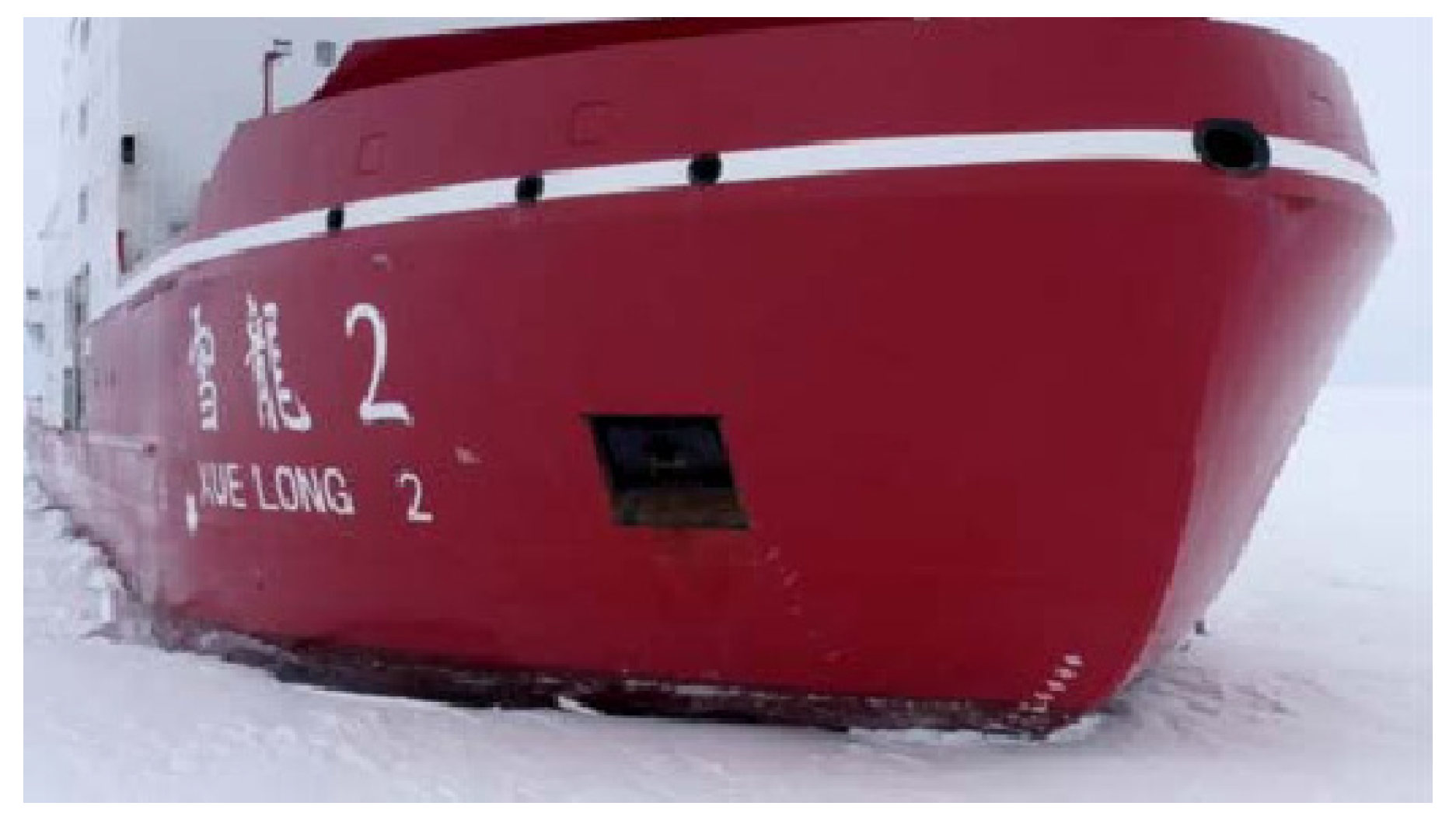
3.1.1. The Adopted Ship Structure

To illustrate the proposed framework (Figure 1), a numerical example corresponding to the PC-2 icebreaker ramming first-year ice ridge is studied. Since the bow is the main part that interacts with ice ridge, the main structural damage also occurs in this part. Therefore, the bow of the PC-2 icebreaker is chosen for ice-load simulation and structural analysis, as shown in Figure 2.

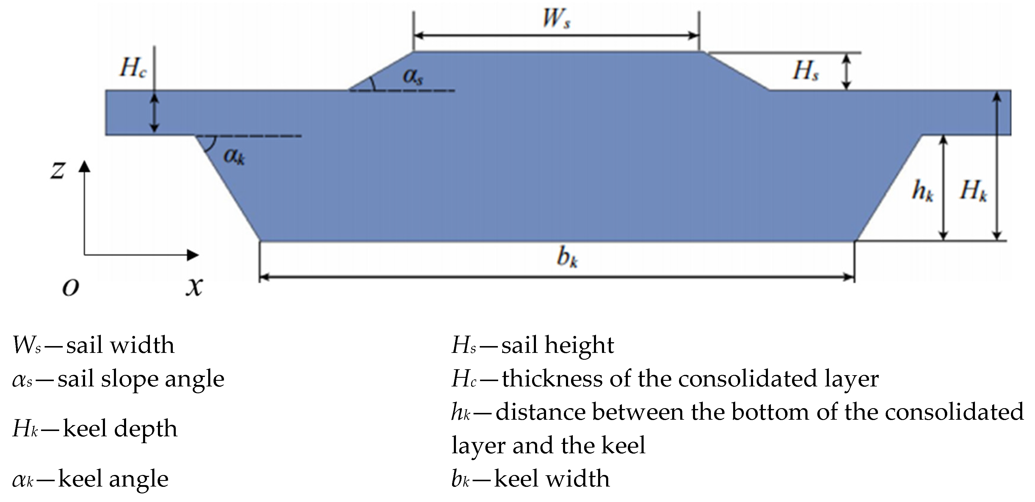
3.1.2. The Morphology and Main Dimensions of First-Year Ice Ridges

An ice ridge is composed of sail and the keel. The keel in first-year ridges consists of an upper consolidated layer and a lower unconsolidated layer (the rubble). Both the sail and the rubble consist of loosely connected pieces of ice whereas the consolidated layer is refrozen and solid and is similar to level ice. The key geometrical parameters of ridges are the keel depth, the thickness of the consolidated layer, the sail height, the keel width, the keel shape, and possibly the block thickness, where the keel depth and the consolidated layer are the two most important parameters of ridge loads (Figure 3).
The sail height provides some valuable information about the feature of an ice ridge. The sail height ratio (keel depth/sail height) for first-ice ridges is about 4~5. The keel width is about 2–3 times the sail width.
The geometry and morphology of the ice ridges are taken from a ridge mapped by Høyland [20] in the North-western Barents Sea (Table 1). Furthermore, the width of an ice ridge is an important factor which affects the ‘passability’ of icebreakers. This quantity is set in Section 4.3 to account for the 3D effects.

3.2. The Ship–Ridge Interaction Model

3.2.1. The Numerical Models for Ice Ridge

To analyze the effect of ice-ridge model, four different ice-ridge models were set up in this work, as shown in Table 2.
In Table 2, the model A sets the whole first-year ice ridge (including the sail, consolidated layer, and keel, ref Section 3.1.2) as a homogenous continuous surface cap (CSCM) model (MAT 145 in LS DYNA, version: R11.0 MPP). This model was earlier used to model a first-year ice ridge by [13] and is coupled with a continuum-damage-mechanics formulation to provide strain-softening feature.
The Model B sets the whole first-year ice ridge (including the sail, consolidated layer, and keel) as an elastic–brittle model; the elastic modulus and maximum failure criterion need to be determined. When the strain of element reaches the maximum failure strain of the elastic–brittle model, the element will be removed. The elastic–brittle model for ice has been corroborated experimentally by numerous researchers [21,22,23] and has high computational efficiency.
Model C sets the consolidated layer as an elastic–brittle model that is the same as that of Model B, whereas the sail and keel are modelled using CSCM with weak strength parameters.
The Model D sets the consolidated layer as a CSCM model that is the same as that of Model A, whereas the sail and keel are modelled using CSCM with weak strength parameters. For model details, refer to Appendix A.1. The employed parameters for the CSCM and elastic–brittle model are given in Appendix A.2.
Since this work mainly focus on the framework for structural analysis of icebreakers during ramming of first-year ice ridges, the material model of an ice ridge is not discussed here; one can also adopt other ice-material models of the ice ridge based on the specific scenario.

3.2.2. The Numerical Setup for Ship–Ridge Interaction

An icebreaker of the PC-2 ice class was employed for the ship–ice interaction analysis. The principal dimensions of the PC-2 icebreaker are presented in Table 3. The bow of the icebreaker is modeled by means of rigid shell elements, the ice ridge is discretized by means of solid elements, as shown in Figure 4.
The morphology of the ice ridge in Figure 3 was applied in the ship–ice interaction analysis. The length (in y-direction) of the ice-ridge model is 80 m, which is almost 4 times the hull width. To obtain convergent results while retaining a reasonable CPU time, the element mesh of the level ice is set to 400 × 400 × 400 mm3. The degrees of freedom in the x and y directions (the coordinate system is defined in Figure 4) at the ice boundary are fixed. The ship speed is set as 3 kn (constant speed).
The large deformation when the ship penetrates the ice ridge was simulated by the element-erosion technique (CONTACT_ERODING_SURFACE_TO_SURFACE for the contact between the ship and the ice ridge, and CONTACT_ERODING_SINGLE_SURFACE for ice ridge alone [24]. The ship–ice friction coefficient was set to 0.15 [25].
The effect of sea water on the behavior of the ship and the ice ridge was simulated with the Arbitrary Lagrangian Eulerian (ALE) approach. The equations of state (EOS) and material models for sea water and air are implemented. An EOS according to the Gruneisen model is suggested to simulate fluid domains in the current FE solver [26]. The numerical set up for analysis of ship–ice interaction is shown in Figure 4a, the displacement and rotation angle at the edge of ice ridge are fixed in the simulation setup (Figure 4b). The preliminary results related to the effects of the water on the ship and the ice ridge can be seen in Figure 5. It is observed that the bow of the icebreaker creates waves, and that the waves are acting on the ice ridge.

3.3. The Validation of Ship–Ridge Interaction Model

Based on the simulation of ship–ice interaction, the ice resistance (resultant force) for ship-ramming of a first-year ice ridge can be obtained, as shown in Figure 6.
It can be seen from Figure 6 that the ice resistance shows an increasing trend as the icebreaker progresses during Phase I. The contact area gradually increases during the time interval from 0 to 8 s. After 8 s, most of the bow part has entered into the ice ridge and the ice resistance fluctuates within a relatively stable range during Phase II. Therefore, the ice-load data during Phase II is averaged to represent the ice resistance, which is compared with experimental values found in the literature [27]. It is also worth noting that the ice resistance decreases when the bow part gradually crosses the ice ridge, as shown in Figure 7a. This is because the flexural failure of the consolidation layer of ice ridge causes boundary element failure (Figure 7b), which in turn causes the ice resistance to decrease. As the bulk of the bow structure enters the ice ridge, the ice resistance remains relatively constant as the overall contact area remains constant.
Wu et al. [27] examined the ice-breaking capability of R/V Xuelong 2 under full-scale conditions. A series of tests were carried out in the fast-ice area near Zhongshan Station in the Prydz Bay during the maiden Antarctic voyage of R/V Xuelong 2 (Figure 8). During the in situ tests, R/V Xuelong 2 navigates at a speed of 0.9~6 kn in a level ice field. The average ice thickness of the level ice field is 1.4 m ± 0.2 m.
The Lindqvist formulation is an engineering tool for the evaluation of ice resistance [28]. In this work, The Lindqvist solution is compared to the simulated ice resistance. The detailed Lindqvist formulas are given in Appendix A. Table 4 presents the employed ship and ice parameters presently being input to the Lindqvist formulation. The obtained ice resistances based on the Lindqvist formulation and the related parameters are shown in Figure 9.
In Figure 9, the simulated ice resistance obtained based on the ship–ridge interaction is compared with results from the in situ tests of Xuelong 2 and with the Lindqvist solution. The consolidated layer of the ice ridge can be considered as being equivalent to level ice, and the thickness of the equivalent level ice will then have a value bounded by 1.5 m and 2.5 m. Therefore, these two values of the ice thickness are employed as inputs for the Lindqvist formulation. Although the sail is modeled in Figure 7a, the material properties of sail is weak, it contributes little to the total ice resistance.
It can be seen from Figure 9 that the simulated ice resistance at a speed of 3 kn is almost 3600 kN, which lies between the values obtained from the Lindqvist formulation with H = 1.5 m and the Lindqvist formulation with H = 2.5 m. The ice resistance obtained by numerical simulation is around 3600 kN, which is more than twice the experimental value of Xuelong 2 (about 1500 kN). Furthermore, the ice resistance obtained by Lindqvist solution with 2.5 m thickness ice is almost two times the ice resistance obtained by numerical solution in this work. The difference is due to the consolidated layer contributing the most to the ice resistance, while the sail and keel contribute little to the ice resistance. The thickness of consolidated layer is 1.5 m, which is closer to the half of 2.5 m. Therefore, the ice resistance obtained by numerical simulation is lower than that of Lindqvist solution, with 2.5 m thickness.
It is worth noting that the in situ tests of Xuelong 2 were carried out in the Antarctic. Reference [29] showed a significant difference in the spatial scale of the variability of sea–ice properties between the Arctic and Antarctic; this difference could cause different ice resistance on the icebreaker. Furthermore, the main dimensions of Xuelong 2 are different from those of the adopted PC-2 icebreaker. In particular, the width of Xuelong 2 is around 22.3 m, while the width of the adopted PC-2 icebreaker is 29 m. The difference in the main dimensions of the ship also contributes to the discrepancy in the results for the ice resistance.
In general, the ice resistance obtained by the numerical simulation in this work is within a reasonable range. The difference in ice resistance between the in situ tests and the numerical simulation is caused by many effects, such as ice type, ice properties, ship dimensions, etc. Furthermore, the simulated ice resistance is close to that of the Lindqvist formulation, which also may support the simulated ice resistance. As for the employed PC-2 icebreaker in this work, it is still at the design stage, so the experimental data of the as-built PC-2 icebreaker is not available currently. Due to the lack of experimental data of ship ramming ice ridge, the current numerical results can not be verified by in situ tests.
It is also worth noting that the ice resistance obtained by the numerical simulation in this work is consistent with the Lindqvist formulation when the ice thickness is 2.0 m. This implies that the target ice ridge can be taken as level ice characterized by the equivalent ice thickness.
Niiler [30] compared the ice resistance calculated using an equivalent ice thickness with the actual resistance measured onboard a ship. He defined equivalent ice thickness as
H v = c ( h i + ( 1 ρ p ) μ h k 2 tan α k + k s n h s n )
where c is the ice concentration; hi is the thickness of the level ice, in m; ρ p is the porosity of the unconsolidated ice rubble in the ridge; μ is the frequency of occurrence of ridges within the ice field, in m−1, assumed as 1/(ridge width) in this work; hk is the ridge keel height; ksn is the snow resistance coefficient; hsn is the snow cover thickness, in m; α k is the base angle of ridge keel.
Adopted parameter values applied in Equation (1) are shown in Table 5. The equivalent ice thickness Hv for the target ice ridge can then be obtained. The obtained value of Hv is 2.05 m which is close to the equivalent ice thickness (almost 2.0 m) in Figure 9.

4. Local Loads and Structural Response

4.1. Local Models for the Structural Analysis

Since the bow is the main area affected by the sea ice, a local model of the bow (extract from left side of real icebreaker) with a refined element mesh was built for the purpose of structural analysis, as shown in Figure 10.
For the local structural part, an elasto-plastic material model was adopted. When the plastic strain reaches the maximum effective plastic strain (around 0.35), the corresponding element of the local structure is deleted from the calculation. The adopted material parameters for the local structure are shown in Table 6.
In order to verify the material model for the local structure, a tensile simulation was carried out and compared with corresponding tensile tests [31]. A series of tensile tests at low temperatures were carried out in our previous work [32]. Zhao et al. [32] studied the mechanical properties of marine DH36 steel within the temperature range from −60 °C to 10 °C. The specimen and the corresponding schematic diagram are shown in Figure 11a and Figure 11b, respectively. Results from the tensile simulation based on the material parameters in Table 6 were compared with related test data from the work of Zhao et. al. [26]. In Figure 12a, the stress and strain in the middle region of the tensile model, then the stress–strain curve can be obtained. A comparison of the stress-strain curve from the simulation versus the test is shown in Figure 12b. It is seen that the adopted material model performs well with respect to tensile behavior at −60 °C. Hence, the elasto-plastic material model with related material parameters in Table 6 is employed in the structural analysis. Furthermore, large deformations are represented within the Total Lagrangian Description (TLD) framework.

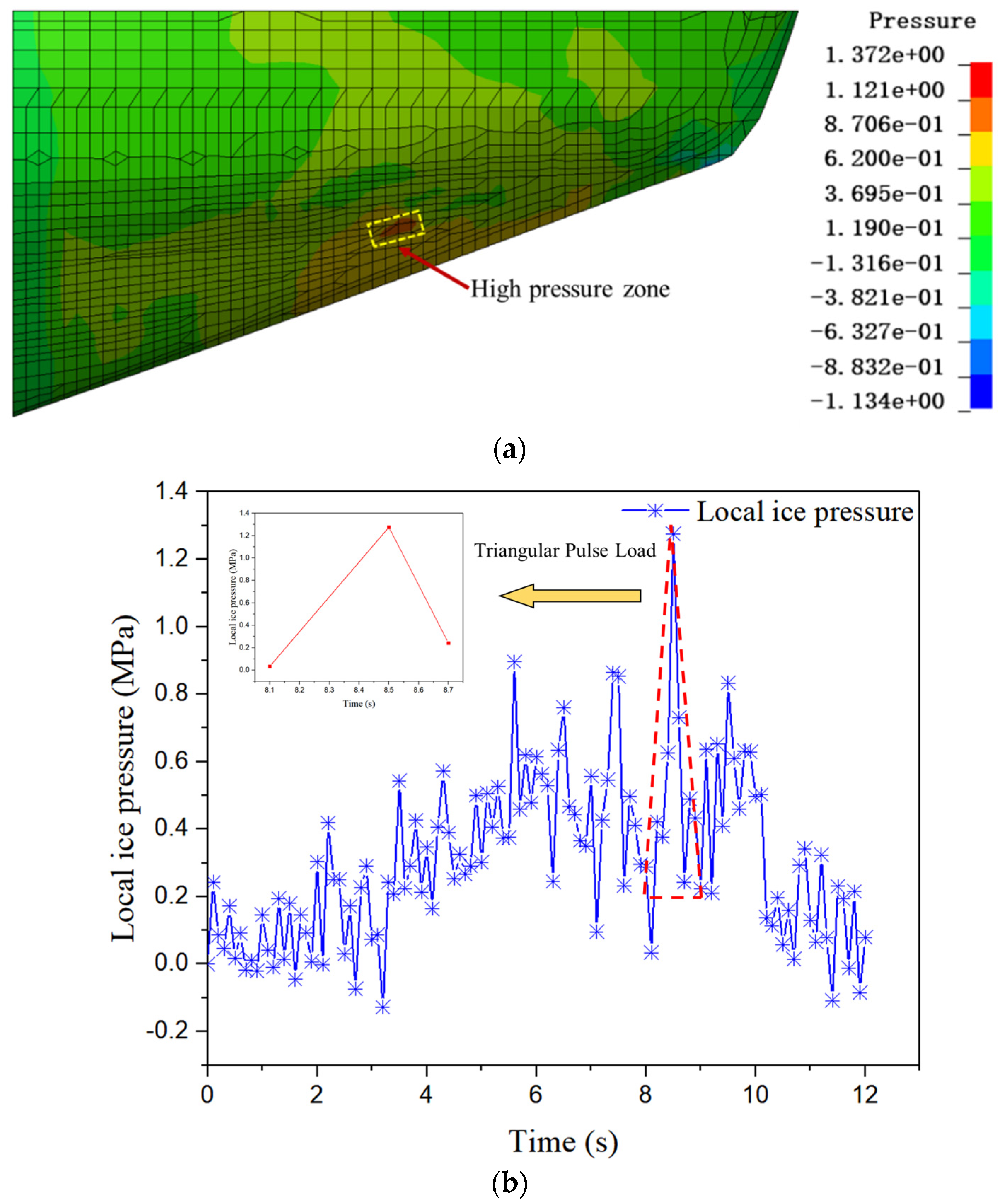
4.2. The Applied Ice Pressure on Local Ship Structures

Based on the numerical model in Section 3.1, the ice load induced by the ridge can be simulated. Figure 13 shows the failure pattern of the ice ridge. It can be seen from Figure 13b that crushing failure mainly takes place during the interaction process.
The local ice pressure acting at the hull in the bow area can be obtained as represented by the local contact pressure, PL. The time–space dependency of the local contact pressure is predicted in this work. For a target monitoring point, the current simulation can predict the time variation of the local contact pressure. Furthermore, the time history of the ice contact pressure at any specified monitoring point can be predicted. For the purpose of simplification, the high-pressure zone (HPZ) is chosen to illustrate the results obtained by application of the proposed framework, as shown in Figure 14. Subsequently, the local contact pressure is applied to the corresponding part of the local model of the ship hull. It is worth noting that the load-patch size applied in the structural analysis corresponds to the HPZ in the present analysis.
It is worth noting that the local ice pressure is not the ultimate ice pressure whose maximum value is around 5~80 MPa [5]. In this work, the peak ice-pressure history (around 8 s in Figure 14b) was extracted and translated into a triangular pulse load.

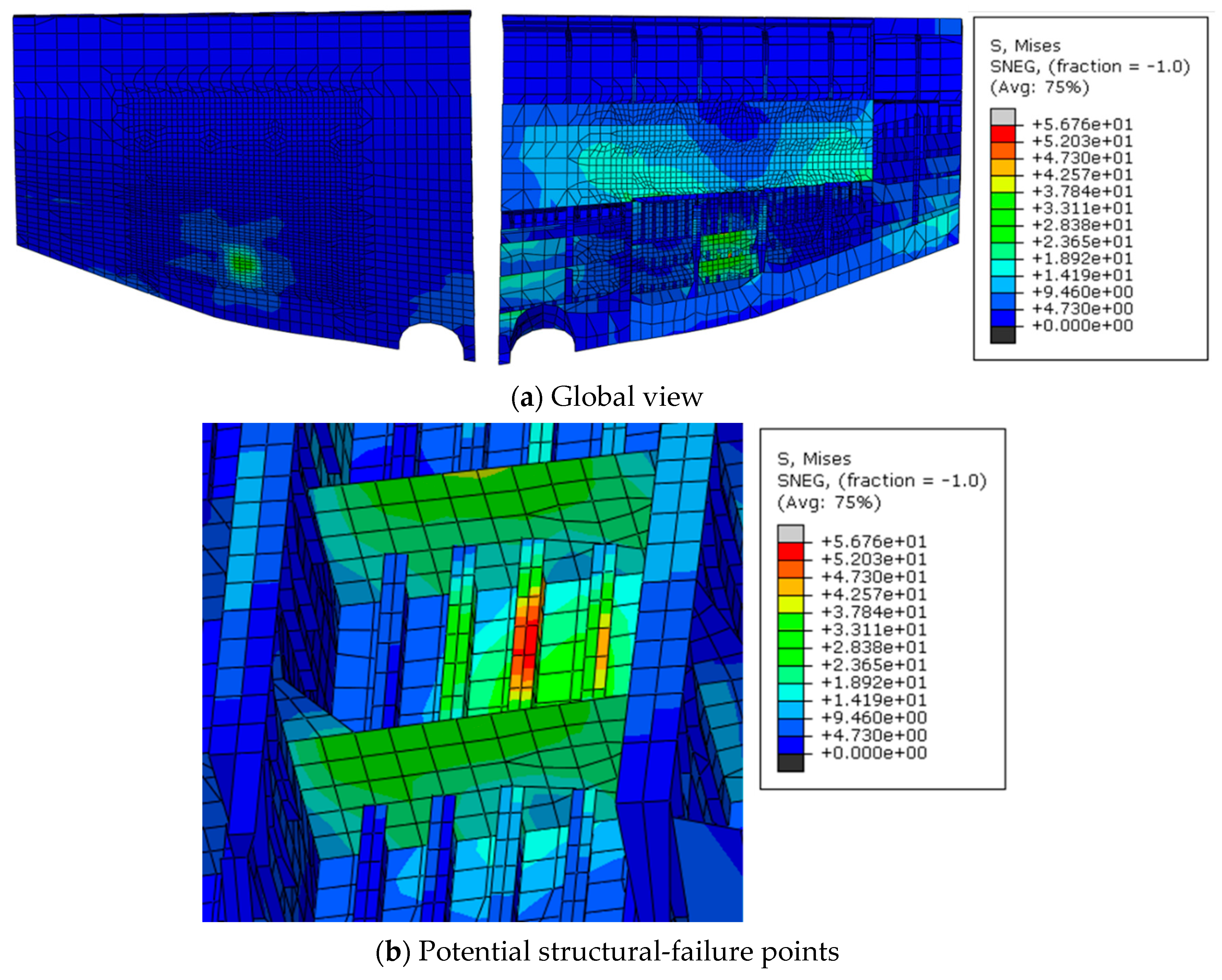
4.3. The Structural Analysis of Local Ship Structures

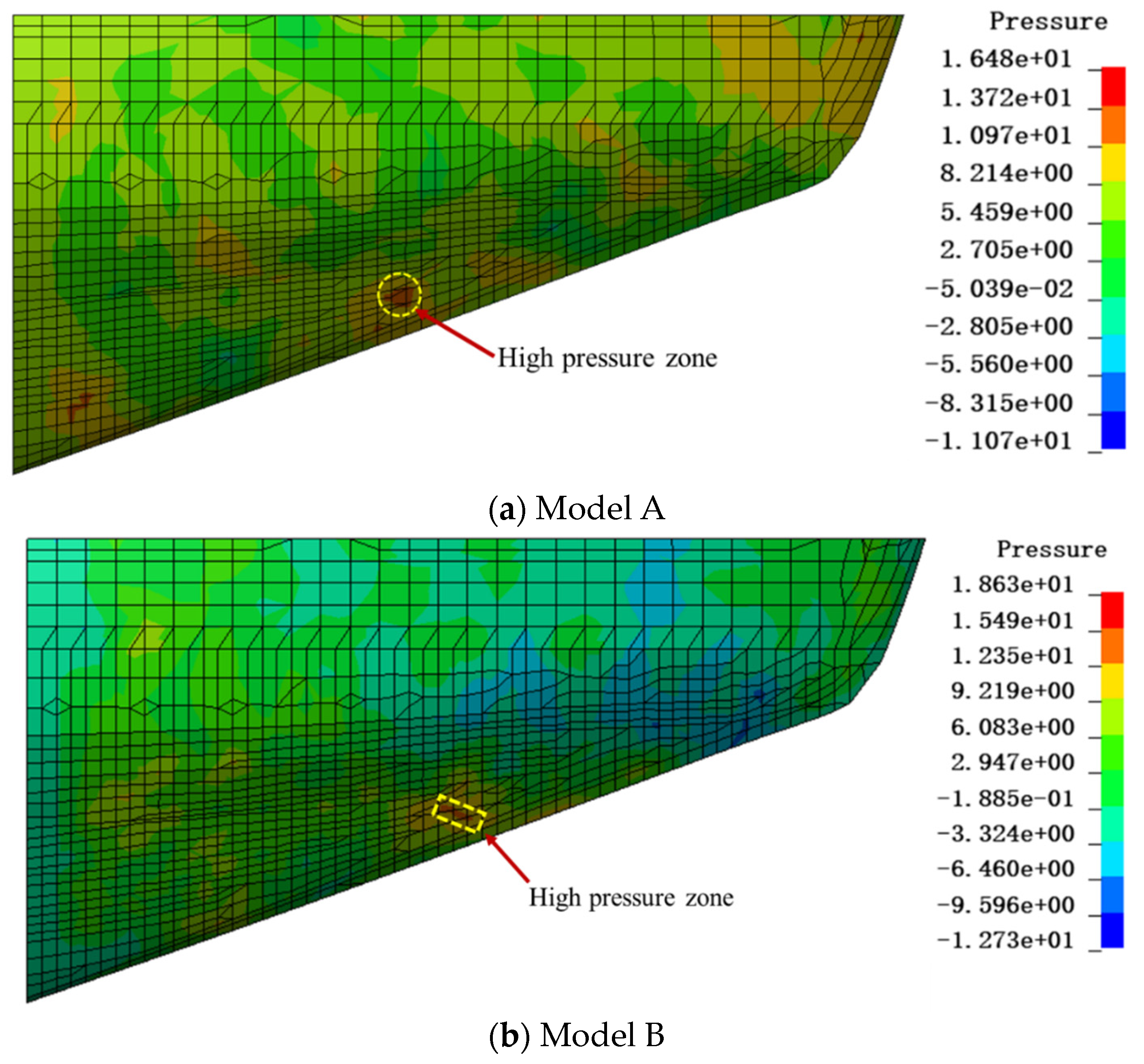
4.3.1. The Design Ice Pressure Based on Ship–Ridge Interaction

The triangular pulse load in Figure 14 is then applied to the local ship sub-structural model, as shown in Figure 15. The degrees of freedom in the x, y and z directions at the boundary of the local model are fixed, as shown in Figure 15a. The load area in Figure 15a is chosen based on the ship–ice interaction event that gives rise to the highest stresses (Von Mises stress in the local substructural models of the hull). Figure 15b illustrates the extension of the load patch (3.2 m × 2.2 m) which corresponds to the contact area.
Based on the dynamic structural analysis, the corresponding response in terms of von Mises stress level was obtained, as shown in Figure 16a. Figure 16b shows the potential structural-failure points located at the backside of the loaded area. The shell side longitudinal in Figure 16b bends under the external ice pressure, and this gives rise to high stress levels.
Figure 17 shows the strain-energy density within the local sub-structure. It can be seen from this figure that the strain energy is continuously rising during the loading stage and reaches its peak at around 0.45 s. After that, the strain energy decreases and approaches zero which means that only elastic processes take place due to the present impact loading.

4.3.2. The Ice Pressure under Dangerous Scenario

Considering the extreme ice pressure (5~80 MPa) that is acting on the local structure, a corresponding stress-response analysis of the local sub-structure is carried out. According to ISO 19906 [5], the ice pressure on local areas can increase to a level around 25 MPa to 40 MPa. Here, a 25 MPa ice pressure is applied on local ship hull components, and the resulting stress distribution for the local structural model is shown in Figure 18. It can be seen from this figure that plastic deformations take place in parts of the sub-structure. The peak of the induced von Mises stress is around 515.1 MPa, which exceeds the yield strength of the ship hull material (384.5 MPa).
Figure 19 presents a comparison between the two loading scenarios. It is obvious that the strain-energy density corresponding to PL = 25 MPa is almost 1000 times the strain-energy density for the case with PL = 1.27 MPa. In general, the assumed ultimate state can represent a critical condition for the target local sub-structures.

5. Discussion

5.1. The Comparison of Different Ice Ridge Material Models

The results in Appendix A.2.1 show that the elastic material model exhibits a good performance for the undamaged state when performing simulation of uniaxial compression of the ice ridge. Hence, the elastic material model is also employed for the purpose of analyzing the effect of the ice material model on the ship–ice interaction process (corresponding to model B below).
Furthermore, in the above analysis based on the inelastic CSCM model, the ice ridge was represented as having different material properties for the different parts of the ice ridge. This is referred to as model D in the analysis below. As an alternative simplified model, the ice ridge is set as having uniform material properties, and the CSCM is deployed with the parameters presented in Table A2 (in Appendix A.2.1), as shown in Figure 20. This model is referred to as model A in the analysis below.
Based on four different ice-ridge models (A, B, C and D), a comparison between the results obtained by application of the different models is obtained.
Model A. The whole ice ridge was modeled as a CSCM material (homogenous).
Model B. The whole ice ridge was modeled as an elastic material.
Model C. The materials of the consolidated layer and the keel were represented by the elastic model and the CSCM material, respectively.
Model D. The materials of the consolidated layer and the keel (sail) were represented by different CSCM models.
Based on the four ice-ridge models, the corresponding pressure contours for the ship hull structure can be obtained, as shown in Figure 21 (The pressure contour of Model D is already given in Figure 14a). For the four ice-ridge models, the obtained characteristics of the local ice pressure within the HPZ are listed in Table 7. It can be seen from Table 7 that there is a clear difference between the characteristics of the local ice pressure corresponding to the four ice-ridge models.
Comparison between the peak ice pressure and the maximum von Mises stress within the local sub-structure is shown in Figure 22. These two quantities exhibit a similar trend when comparing results from the three different models. It can be seen from Figure 22 that the peak ice pressure and maximum von Mises stress obtained by Model A and Model B are obviously higher than those of Model C and Model D. Model A and Model B lead to a higher lower-peak pressure and maximum stress than Model C and Model D. This is due to the fact that Model A and Model B represent the keel part with the same mechanical properties as the consolidated layer. From the perspective of polar ship design, Model A and Model B could be good choices since the structural response obtained by these models is most likely higher than the actual value, which implies a certain safety margin. Model C and Model D are still suitable for structural assessment of polar structures for certain ice conditions.
Figure 23 shows the comparison of the strain-energy density among the three models. Similar to the trend for the peak stress, the strain-energy density predicted by Model A and Model B is higher than that of the two other models. Model D results in the lowest strain-energy-density value. Furthermore, the time span of the strain-energy density for the four ice-ridge material models is also different. The span value is related to the load period in Table 7.

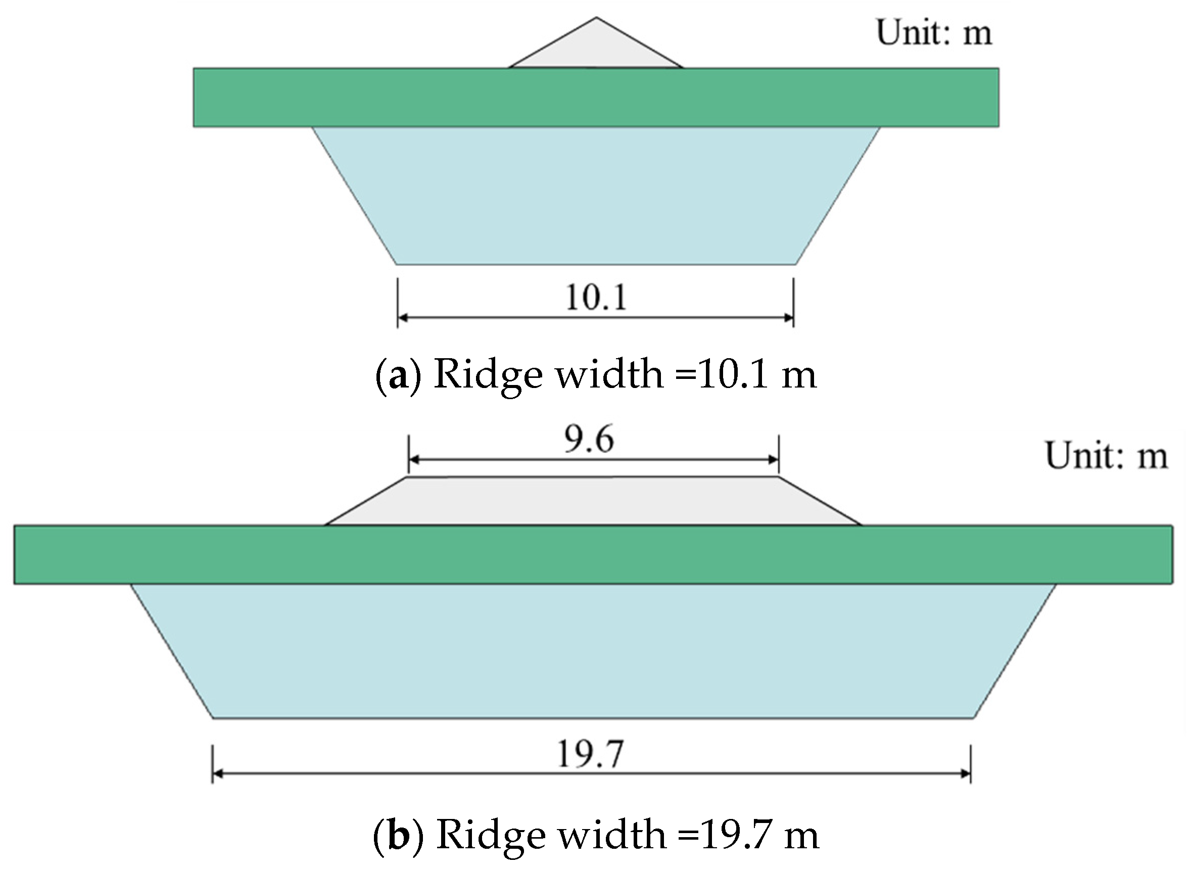
5.2. The Effect of Ridge Width on Structural Response

The results given in Ref. [7] show that the ridge width has a significant effect on the ridge resistance. In this work, the effect of varying ridge widths on the structural response is discussed. The ridge width (keel width in this work) is set as 10.1 m, 19.7 m, and 28.7 m for the three different cases to be analyzed (see Figure 24).
Figure 25 shows the simulated ridge resistance of the icebreaker for different ridge widths. It can be seen from Figure 25 that the simulated ice resistance for the three ridge widths show good consistency up to 7.2 s. The simulated ice resistance for a ridge width of 10.1 m reaches its peak at around 7.2 s. After that, the ice resistance decreases since global bending failure of the ice takes place. The ice resistance for the other two ridge widths reaches its peak at 8.6 s and 12.8 s, respectively. Figure 26 shows the simulated peak ridge resistance of the icebreaker as a function of the ridge width. For the PC-2 icebreaker employed here, the peak ridge resistance increases when the ridge width increases.
Table 8 presents the local contact pressure for different ridge widths. It can be seen from this table that the peak pressure in the HPZ for a ridge width of 10.1 m is lower than that for a ridge width of 19.7 m and for a ridge width of 28.7 m. Still, there is little difference between the peak pressure for a ridge width of 19.7 m and a ridge width of 28.7 m. The size of the HPZ increases for increasing ridge widths. The load period does not show any clear trend as a function of the ridge width.
Figure 27 presents the structural response for different ridge widths. Figure 27a shows that the maximum structural stress for a ridge width of 10.1 m is significantly lower than for the cases with a ridge width of 19.7 m and with a ridge width of 28.7 m (still the peak pressure is almost the same for these to latter cases). This trend is consistent with the fact that the peak ridge resistance changes with the ridge width.
In Figure 27b, the span of the strain-energy density curves for different ridge widths is consistent with the respective load periods in Table 8. The peak value of the strain-energy density also exhibits the same trend for increasing ridge widths. In general, the peak ridge resistance, the peak pressure at the HPZ, the maximum structural stress and the peak strain-energy density show the same trend for increasing the ridge widths.

5.3. The Effect of Ship Speed on Structural Response

According to the “Polar Ship Guide” published by China Classification Society (CCS) [33], the recommended speed limit for a PC-2 icebreaker is 8 kn. Hence, an 8 kn speed limit is chosen to study the effect of ship speed on the absorbed strain energy.
Figure 28 shows the failure pattern for the ice ridge based on this speed. It is found that the crushing failure mainly occurs during the ship–ridge interaction process. Table 9 presents the local contact pressure corresponding to different ship speeds. The size of the HPZ and the peak pressure in the HPZ for the case with a speed of 8 kn are both larger than the values for a speed of 3 kn, while the load period for a speed of 8 kn speed is shorter than that for a speed of 3 kn.
Based on the simulated ice pressure at HPZ, the structural analysis is carried out, as shown in Figure 29. The peak structural stress for a speed of 8 kn is around 433.8 MPa and located at the frame behind the HPZ. The peak structural stress at 8 kn is significantly higher than at 3 kn (for which it is around 56 MPa).
The obtained strain-energy density for a local sub-structure corresponding to a speed of 8 kn is compared with that for a speed of 3 kn, as shown in Figure 30. Apparently, the strain-energy density at 8 kn is much higher than that at 3 n. Furthermore, the time span of the strain-energy density for the two speeds is also different, which is related to the associated load period. In general, ship speed has a significant effect on the structural response of ship structures during ramming of first-year ice ridges.

6. Concluding Remarks

The determination of ice-ridge forces on ships in relation to ship strength is of significant practical importance in relation to the safety and economy of icebreakers sailing in ice-covered regions. A framework for the structural analysis of icebreakers ramming first-year ice ridges is proposed in this work. An application example illustrating structural analysis of an icebreaker during the ramming of a first-year ice ridge is carried out according to the proposed framework. The obtained results lead to the following conclusions:
(1) Four ridge models are introduced in this work. Among them, the simulation efficiency of model B is much better than it is for the other models since it requires few material parameters. Model D can simulate the situation after ice ridge failure but requires a large number of material parameters.
(2) The strength of the keel is lower than that of the consolidated layer of the ice ridge. It is recommended to differentiate between the material parameters of the keel and the consolidated layer when analyzing the structural response of ship structures ramming into ice ridges, while a homogeneous ice-ridge model could be an adequate choice for strength design of other types of structures in polar areas.
(3) The width of the ridge affects the ice resistance and the structural response of polar ship hulls. The peak ice resistance, peak structural stress, and strain-energy density increase with increasing widths of the ridge.
(4) Ship speed has a significant effect on local ice loads and structural response. The strain-energy density that is obtained for the case with 8 kn speed is clearly higher than that obtained for the case with 3 kn speed. Safe ship-speed design deserves to be studied as part of future work in this area.
Furthermore, due to the lack of in situ data on the collision between ships and ice ridges, the results from the present study cannot be compared with measurements of ice-ridge forces acting on the hull surface. Rather, the objective has been to provide a comparative study between results obtained for the different cases. Verification and possibly calibration of the present calculation models should be carried out as part of future research work. The local ice pressure has strong randomness, which will be analyzed by means of probabilistic methods as part of future studies.

Author Contributions

Conceptualization, B.J.L. and K.V.H.; methodology, W.Z.; software, W.Z.; validation, W.Z. and E.K.; formal analysis, B.J.L.; investigation, K.V.H.; resources, E.K.; data curation, G.F.; writing—original draft preparation, W.Z. and E.K.; writing—review and editing, B.J.L. and K.V.H.; visualization, E.K.; supervision, G.F. and H.R.; project administration, G.F.; funding acquisition, G.F. All authors have read and agreed to the published version of the manuscript.

Funding

This paper was supported by the Shandong Provincial Natural Science Foundation (Fund No. ZR2022QE092) and the National Natural Science Foundation of China (Fund No. 52171301) China Postdoctoral Science Foundation (Grant No. 2023M730829).

Institutional Review Board Statement

Not applicable.

Informed Consent Statement

Not applicable.

Data Availability Statement

Data are contained within the article.

Conflicts of Interest

The authors declare no conflict of interest.

Appendix A. The Material Model of Ice Ridge

Appendix A.1. The Continuous Surface Cap Model

At present, there does not exist any perfect ice material model due to the complex physical properties and microstructure of ice. In this work, the CSCM is employed for the material found in consolidated ice ridges. Within the proposed framework, it is also possible to implement alternative material models for the ice.
The CSCM model provided reasonable results for the purpose of demonstration of the proposed framework. Note that the framework is not limited to this particular modelling technique and there are other ways of modelling ice ridges.
As for the CSCM, this material model is a smooth or continuous surface cap model and is available for solid elements. Furthermore, the damage during the post-failure stage was also embedded in the CSCM based on a Continuum Damage Mechanics model [24].
The CSCM model is based on the work of Lemaitre [34] and Dufailly and Lemaitre [35]. The failure surface of the smooth cap model is defined as
F f ( J 1 ) = α λ exp ( β J 1 ) + θ J 1
where J1 is the first invariant of the deviatoric stress tensor; and α, θ, λ, and β designate model parameters used to match the triaxial compression. The isotropic hardening or cap surface of the model is based on a nondimensional functional form
F c ( J 1 , κ ) = 1 [ J 1 L ( κ ) ] [ | J 1 L ( κ ) | + J 1 L ( κ ) ] 2 [ X ( κ ) L ( κ ) ] 2
where κ denotes the hardening parameter that controls the motion of the cap surface, and L(κ) and X(κ) define the geometry of the cap surface. The smooth cap model, shown in Figure A1, is formed by combining the failure and hardening surface functions to form a smoothly varying function given by
f ( J 1 , J 2 , κ ) = J 2 F f 2 F C
where J 2 denotes the second invariant of the deviatoric stress tensor.
Figure A1. The shear surface of the CSCM material model (The pressure is a hydrostatic pressure which is equal to σ 1 + σ 2 + σ 3 3 ) [36].
Jmse 12 00611 g0a1
Considering the complex morphology and properties of ice ridges, an equivalent ice-ridge model applying the CSCM material model is employed in this work.
The softening mechanism of the CSCM model in the tensile and low-to-moderate compressive regimes is accounted for by the following expression [24]:
σ i j d = ( 1 d ) σ i j v p
Here, a scalar damage parameter, d, transforms the viscoplastic stress tensor without damage, denoted σ v p , into the stress tensor with damage, denoted by the superscript d. Damage accumulation is based upon two distinct formulations, which we call brittle damage and ductile damage. The initial damage threshold is coincident with the shear plasticity surface, so the threshold does not have to be specified by the user.
(a) Ductile Damage. Ductile damage accumulates when the pressure, P, is compressive and an energy-type term, τ C , exceeds the damage threshold, τ 0 C . Ductile damage accumulation depends upon the total strain components, ε i j , as follows:
τ C = 1 2 σ i j ε i j
The stress components, σ i j are the elasto-plastic stresses (with kinematic hardening) calculated before application of damage and rate effects.
(b) Brittle Damage. Brittle damage accumulates when the pressure is tensile and when an energy-type term, τ t , exceeds the damage threshold, τ 0 t . Brittle damage accumulation depends upon the maximum principal strain, ε max follows:
τ t = E ε max 2
The viscoplastic rate effect (embedded in the CSCM model) is also consider in this work. At each time step, the viscoplastic algorithm interpolates between the elastic trial stress, σ i j T , and the inviscid stress (without rate effects), σ i j p , to set the viscoplastic stress (with rate effects), σ i j vp [24]:
σ i j vp = ( 1 γ ) σ i j T + γ σ i j p
where
γ = Δ t / η 1 + Δ t / η
This interpolation depends upon the effective fluidity coefficient, η, and the time step, Δt. The effective fluidity coefficient is calculated based on five user-supplied input parameters and interpolation equations:
Tensile   pressure :                 η = η s + J 1 3 J 2 P S T η t η s
Compressive   pressure :                 η = η s + J 1 3 J 2 P SC η c η s
where
η s = R s t × η t
η t = η 0 T ε ˙ N T
η c = η 0 C ε ˙ N C
where,
P S C is the shear-to-compression transition parameter,
P S T is the shear-to-tension transition parameter,
η 0 C is the rate effect parameter for uniaxial compressive stress,
η 0 T is the rate effect parameter for uniaxial tensile stress,
N C is the rate effect power for uniaxial compressive stress,
N t is the rate effect power for uniaxial tensile stress,
R s t is the ratio of effective shear stress to tensile stress fluidity parameters.
When the rate effect is considered in the CSCM model, the main parameters affected by the rate effect should be given, which mainly includes η 0 C , η 0 T , N C , N t . Regarding the tensile behavior, as mentioned above, experimental results show brittle failure and a negligible influence of strain rate on the strength of ice, so the rate effect on the tensile strength of ice is not considered in this work [37].

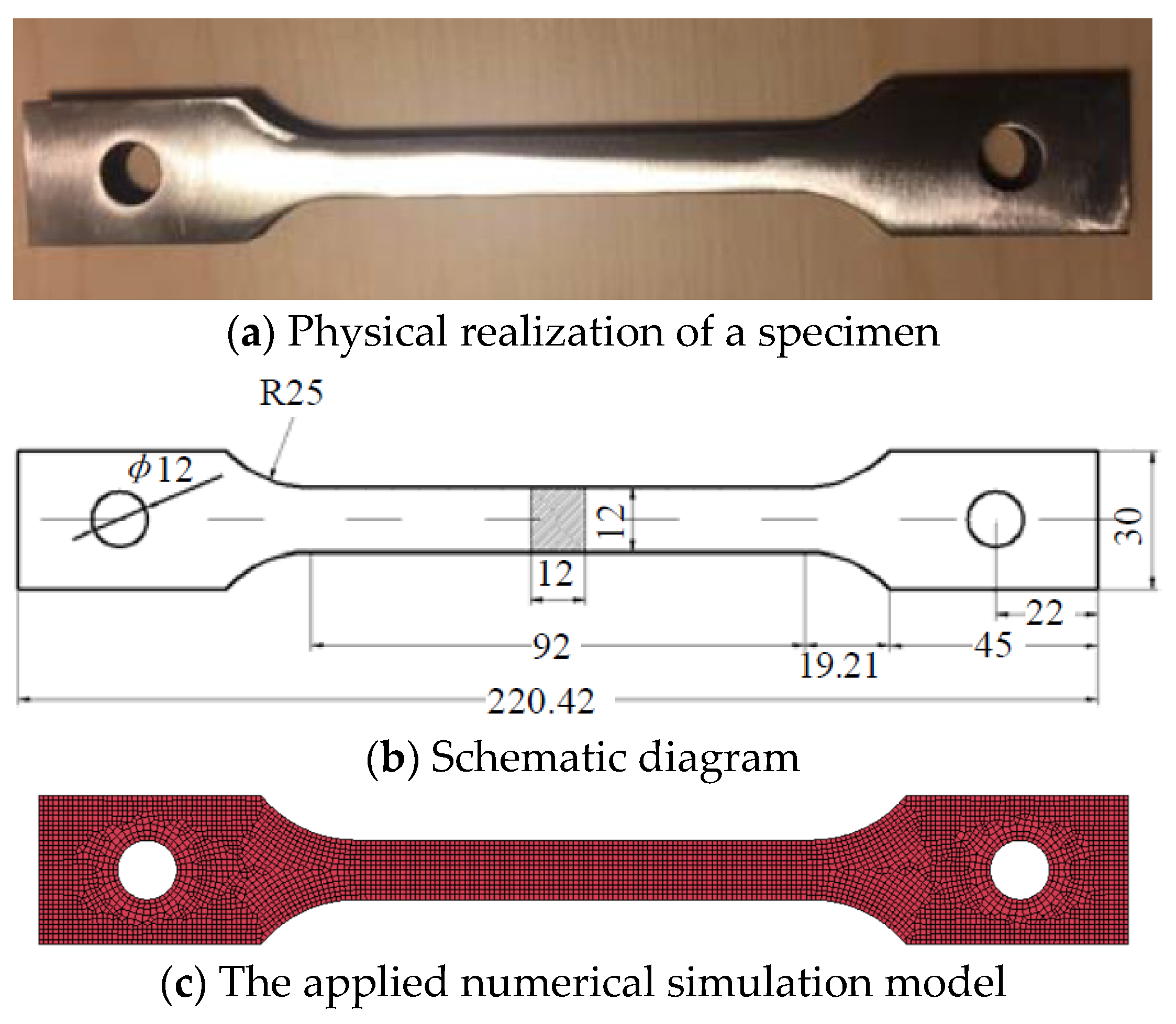
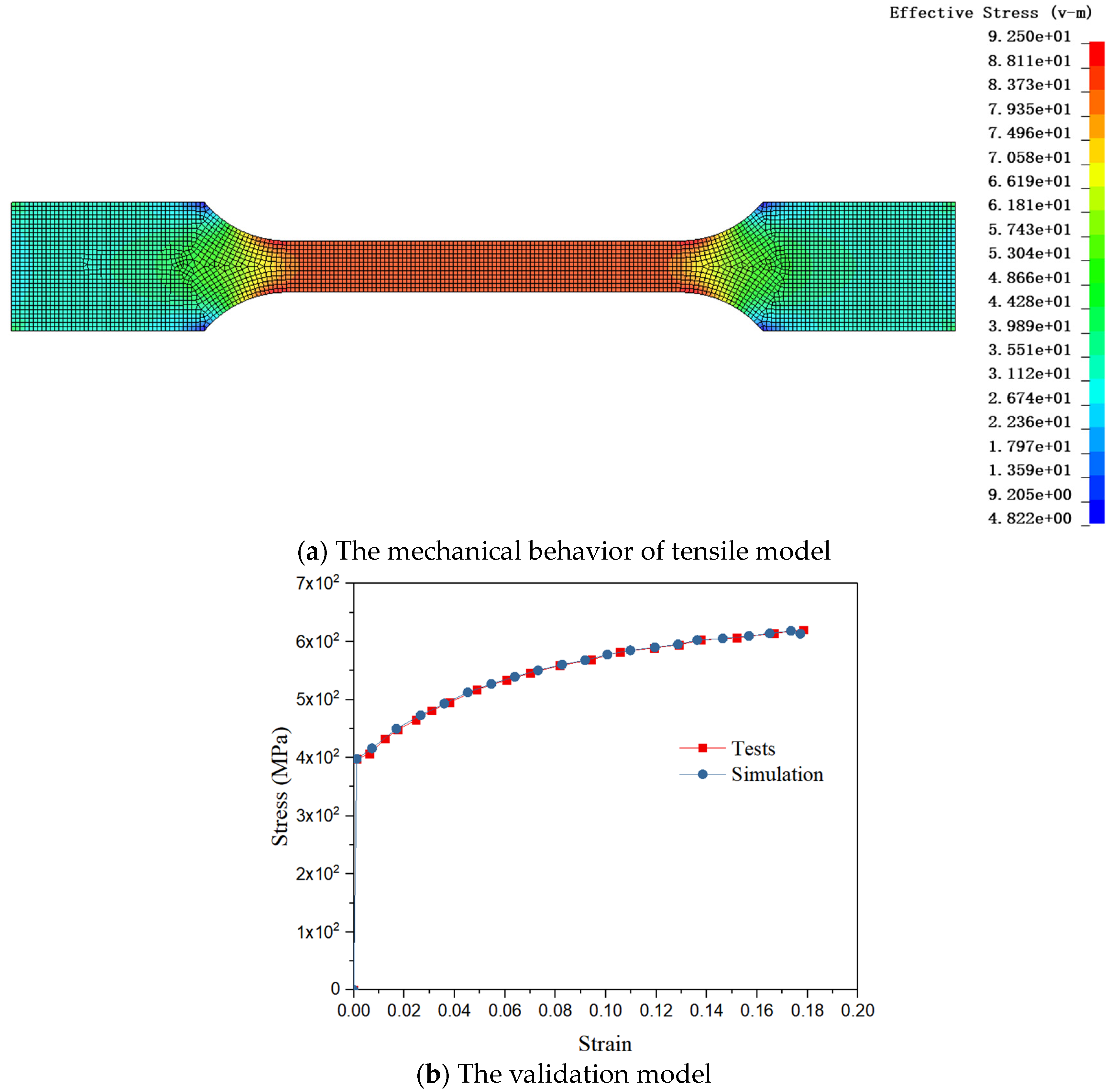
Appendix A.2. The Material Parameters and Validation of Ice Ridge

A considerable knowledge gap was found to exist with respect to the mechanical properties of the consolidated layer of first-year ridges. So far, the most comprehensive studies on the uniaxial compressive strength of ice samples from first-year ridges have been published by Shafrova and Høyland [38]. Table A1 lists the main mechanical properties and ice strength of first-year ice ridges which are obtained based on ref. [20].
Table A1. The main physical and mechanical properties of first-year ice ridges [20].
Consolidated layer (2004 lab tests, Barents Sea)porosity (%)salinity (ppt)density (kg/L)ice strength (MPa)
5~104.40.883.94 (±1.62)
The CSCM material model is employed in order to simulate the properties of the first-year ice ridge. During the ship–ridge interaction process, mainly crushing failure takes place in the consolidated layer of the ice ridge, while shear failure takes place within the keel part. To validate the ice model, uniaxial compression tests of the consolidated layer and punch-through shear tests of the keel are simulated, respectively.
Furthermore, the verification of the ice model is related to the primary failure modes of ice during the process of ship–ice interaction. Within the proposed framework, other types of material verifications can also be accommodated depending on the characteristics of each specific ship–ice interaction scenario. As an example, this may correspond to validation of the crushing and flexural strength properties of level ice when the ship is navigating in a level-ice field.

Appendix A.2.1. Uniaxial Compression Tests for Consolidated Layer of Ice Ridge

As we have primarily focused on compressive behavior of an ice ridge (especially the consolidated part), the ice material model performance is verified against experimental data obtained from uniaxial compression tests in this section.
Bonath et al. [39] carried out 410 small-scale uniaxial compression tests at different strain rates and ice temperatures. The specimens were taken from the consolidated layer of six different first-year ridges in the sea around Svalbard. The physical and mechanical properties of the first-year ice ridges are estimated based on these test results [39].
A uniaxial compression model of the ice is applied to verify the ice material model in this work. According to the research by Bonath [39], the shape of the ice specimens was a rectangular prism with 170 mm height and a square base with 70 mm side length. The same dimensions of the ice specimens are applied here for simulation of compressive strength (Figure A2).
Figure A2. The FEM model for simulating compressive loading.
Jmse 12 00611 g0a2
Table A2. The material parameters of the CSCM applied for the consolidated layer of ice ridge [37,40].
ParameterSymbolValue
Density (Kg/m3) ρ c l 887
Shear modulus (MPa)G1538
Bulk modulus (MPa)K3333
Compression surface termsα1.0
θ0.396
Cap ellipticity ratioR8.957
Initial intercept of the cap surfaceXD10.0
Maximum plastic volumetric strainW0.093
Linear shape parametersD186.0
Quadratic shape parametersD20.03
Ductile shape softening parameterB1.0
Fracture energy in uniaxial compressionGfc0.327
Brittle shape softening parameterD1.0
Fracture energy in uniaxial tensionGfs0.0372
Fracture energy in pure shearGft0.0372
Rate effects parameter for uniaxial compressive stress η 0 C 10.976
Rate effect power for uniaxial compressive stress N C 0.093783
The CSCM ice material model based on the parameters in Table A2 above was applied for the uniaxial compression model. The value of the CSCM material parameters are determined by related field tests of ice ridges (shear modulus) [39] and by empirical values found in the literature (compression surface terms) [40].
For the purpose of comparison, an elastic model based on the maximum effective strain as a failure criterion is also introduced. When the strain in an ice element reaches the ε f max value, the element is deleted, which solves the problem of accounting for large deformations of ice elements.
The non-linear behavior of the ice ridge under compression makes it difficult to determine an elastic modulus by mechanical tests. In the literature, the elastic modulus can be referred to as the effective modulus or tangent modulus [41]. Figure A3 illustrates this concept. The tangent modulus in ref. [39] is employed as elastic modulus in this work. The material parameters in Table A3 are employed for this elastic model.
Figure A3. Typical stress–strain curve for ice under uniaxial compression [39].
Jmse 12 00611 g0a3
Table A3. The material parameters of the elastic model for the consolidated layer of the ice ridge [39].
Density
(kg/m3)
Elastic Modulus (MPa)Poisson’s RatioMaximum Effective Strain at Failure
88721600.35 × 10−5~5 × 10⁻³
The results corresponding to compression for the model of consolidated layer obtained based on numerical simulation above are compared with results from the literature [39], as shown in Figure A4. The stress in Figure A4 is the nominal stress which is equal to Force/Area. It is assumed that the stress state of the consolidated layer corresponds to the undamaged state before the nominal stress reaches the peak, and after that, the consolidated layer enters the damaged state. The comparison between the test data and the model predictions indicates that the CSCM shows good performance when predicting the compressive behavior of the consolidated layer of ice ridge in the undamaged and the damaged state, while the elastic model fails to represent the damaged state of the consolidated layer of the ice ridge.
Figure A4. Comparison between the numerical results versus test data (nominal strain rates ε nom = 10 3 s 1 and ice temperatures T = 3.5   ° C ).
Jmse 12 00611 g0a4

Appendix A.2.2. Punch-through Shear Tests for the Keel of Ice Ridge

The punch-through shear tests were introduced to verify the material model of the keel in the ice ridge. In punch-through shear tests, a plate is pushed down through a pre-cut consolidated layer, forming a plug in the rubble underneath. The consolidated layer beneath the plate is separated from the rest of the keel field to reduce the loading capacity and separate the contribution from the consolidated layer [40]. The material model of the consolidated layer is consistent with Table A2, and the material model of the keel is derived from relevant results found in the literature [40], as shown in Table A4.
Figure A5. Illustration of punch-through shear tests for an ice ridge.
Jmse 12 00611 g0a5
Table A4. The parameters of the CSCM material model for the keel [40].
ParameterSymbolValue
Density (Kg/m3) ρ k 541
Shear modulus (MPa)G17.31
Bulk modulus (MPa)K37.5
Compression surface termsα0.016
θ0.182
Cap ellipticity ratioR9.44
Initial intercept of the cap surfaceXD0.595
Maximum plastic volumetric strainW0.05
Linear shape parametersD10.001
Quadratic shape parametersD20.65
Ductile shape softening parameterB20
Fracture energy in uniaxial compressionGfc0.4
Brittle shape softening parameterD1
Fracture energy in uniaxial tensionGfs0.065
Fracture energy in pure shearGft0.065
Rate effects parameter for uniaxial compressive stress η 0 C 10.976
Rate effect power for uniaxial compressive stress N C 0.093783
Figure A6 presents the punch-through shear-test model represented by means of FEM elements. All parts in Figure A6 are modeled by solid elements with homogenous material models. The sea water is dealt with by means of the Arbitrary Lagrangian Eulerian (ALE) approach, which is designed to simulate buoyancy forces acting on the keel. Nodes at the edge of keel geometry are constrained with respect to any displacement in the horizontal and the out-of-plane direction. The consolidated layer is fixed from the anchor location toward the outward horizontal direction. Figure A6 shows a comparison between results from field tests and the simulation of punch-through shear tests. It is seen that the simulated force obtained by the punch-through shear-test model agrees with the test results, which verifies the material model and the related material parameters.
Figure A6. Verification of material model based on punch shear tests for the ice ridge.
Jmse 12 00611 g0a6

Appendix B. The Lindqvist Formulation for Ice Resistance

The Lindqvist formulation [28] is a commonly used calculation approach for ice resistance in ice-covered areas for icebreakers, as shown in Equations (A14)~(A17).
R c = 0.5 σ H 2 tan ϕ + μ k cos ϕ cos ψ 1 μ k sin ϕ cos ψ
R b = 27 64 σ B H 1.5 E 12 ( 1 ν 2 ) g ρ w ( tan ψ + μ k cos ϕ sin α cos ψ ) ( 1 + 1 cos ψ )
R s = ( ρ w ρ i ) g H B { T ( B + T ) B + 2 T + μ k [ 0.7 L T tan ϕ B 4 tan α + T cos ϕ cos ψ 1 sin 2 ϕ + 1 tan 2 α ] }
R t = ( R c + R b ) ( 1 + 1.4 V g H ) + R s ( 1 + 9.4 V g L )
where,
R c is the crushing resistance,
R b is the bending resistance,
R s is the immersion resistance,
R t is the total resistance,
σ is the bending strength of ice,
H is the ice thickness,
E is the elastic modulus of ice,
ν is the Poisson ratio of ice,
μ k is the friction coefficient associated with ship-ice interaction,
ρ w is the density of sea water,
ρ i is the density of ice,
V is the ship speed,
L is the length of the ship,
T is the draught of the ship,
B is the breadth of the ship,
ϕ is the stem angle,
α is the waterline entrance angle,
ψ is the angle between the surface and a vertical vector, tan ψ = tan ϕ / sin α

References

  1. Xie, C.; Zhou, L.; Ding, S.; Lu, M.; Zhou, X. Research on self-propulsion simulation of a polar ship in a brash ice channel based on body force model. Int. J. Nav. Archit. Ocean Eng. 2023, 15, 100557. [Google Scholar] [CrossRef]
  2. Dong, W.; Zhou, L.; Ding, S.; Wang, A.; Cai, J. Two-Staged Method for Ice Channel Identification Based on Image Seg-mentation and Corner Point Regression. China Ocean. Eng. 2024, 38, 1–13. [Google Scholar]
  3. Zhou, L.; Sun, Q.; Ding, S.; Han, S.; Wang, A. A Machine-Learning-Based Method for Ship Propulsion Power Prediction in Ice. J. Mar. Sci. Eng. 2023, 11, 1381. [Google Scholar] [CrossRef]
  4. Tikanmäki, M.; Heinonen, J. Estimating extreme level ice and ridge thickness for offshore wind turbine design: Case study Kriegers Flak. Wind. Energy 2022, 25, 639–659. [Google Scholar] [CrossRef]
  5. EN ISO 19906:2019; Petroleum and Natural Gas Industries—Arctic Offshore Structures. ISO: Geneva, Switzerland, 2019.
  6. Grevsgård, S.M. Finite Element Simulations of Unconsolidated Keel Actions from First-Year Ice Ridges. Master’s Thesis, Norwegian University of Science and Technology, Trondheim, Norway, 2015. [Google Scholar]
  7. Gong, H.; Polojärvi, A.; Tuhkuri, J. Discrete element simulation of the resistance of a ship in unconsolidated ridges. Cold Reg. Sci. Technol. 2019, 167, 102855. [Google Scholar] [CrossRef]
  8. Timco, G.W.; Johnston, M. Ice loads on the caisson structures in the Canadian Beaufort Sea. Cold Reg. Sci. Technol. 2004, 38, 185–209. [Google Scholar] [CrossRef]
  9. Song, M.; Yuan, W.; Liu, K.; Han, Y. Analysis of Ship Motion in An Ice Ridge Field Based on Empirical Approach. China Ocean Eng. 2023, 37, 912–922. [Google Scholar] [CrossRef]
  10. Su, B.; Riska, K.; Moan, T. A numerical method for the prediction of ship performance in level ice. Cold Reg. Sci. Technol. 2010, 60, 177–188. [Google Scholar] [CrossRef]
  11. Kujala, P.; Tuhkuri, J.; Varsta, P. Ship-Ice Contact and Design Loads. In Proceedings of the International Conference on Ships and Marine Structures in Cold Regions, Calgary, AB, Canada, 16–18 March 1994. [Google Scholar]
  12. Hisette, Q.; Alekseev, A.; Seidel, J. Discrete Element Simulation of Ship Breaking Through Ice Ridges. In Proceedings of the 27th International Ocean and Polar Engineering Conference, San Francisco, CA, USA, 25–30 June 2017; ISOPE-I-17-207, Vol. All Days. Available online: https://onepetro.org/ISOPEIOPEC/proceedings-abstract/ISOPE17/All-ISOPE17/ISOPE-I-17-207/17416 (accessed on 25 June 2017).
  13. Lubbad, R.; Løset, S. A numerical model for real-time simulation of ship–ice interaction. Cold Reg. Sci. Technol. 2011, 65, 111–127. [Google Scholar] [CrossRef]
  14. Su, B.; Riska, K.; Moan, T. Numerical study of ice-induced loads on ship hulls. Mar. Struct. 2011, 24, 132–152. [Google Scholar] [CrossRef]
  15. Kim, J.-H.; Kim, Y.; Kim, H.-S.; Jeong, S.-Y. Numerical simulation of ice impacts on ship hulls in broken ice fields. Ocean Eng. 2019, 182, 211–221. [Google Scholar] [CrossRef]
  16. Jeon, S.; Kim, Y. Numerical simulation of level ice–structure interaction using damage-based erosion model. Ocean Eng. 2021, 220, 108485. [Google Scholar] [CrossRef]
  17. Xue, Y.; Liu, R.; Li, Z.; Han, D. A review for numerical simulation methods of ship–ice interaction. Ocean Eng. 2020, 215, 107853. [Google Scholar] [CrossRef]
  18. Aleksandrov, A.; Matantsev, R. Impulse Model for Estimation of Local and Global ice Loads on Fixed Offshore Ice-Resistant Structures. In Proceedings of the Twenty-fifth International Ocean and Polar Engineering Conference, Big Island, HI, USA, 21–26 June 2015; ISOPE-I-15-440, Vol. All Days. Available online: https://onepetro.org/ISOPEIOPEC/proceedings-abstract/ISOPE15/All-ISOPE15/ISOPE-I-15-440/14833 (accessed on 21 June 2015).
  19. Qu, Y.; Yue, Q.; Bi, X.; Kärnä, T. A random ice force model for narrow conical structures. Cold Reg. Sci. Technol. 2006, 45, 148–157. [Google Scholar] [CrossRef]
  20. Høyland, K.V. Morphology and small-scale strength of ridges in the North-western Barents Sea. Cold Reg. Sci. Technol. 2007, 48, 169–187. [Google Scholar] [CrossRef]
  21. Robin, G.d.Q. Seismic shooting and related investigations. In Norwegian-British-Swedish Antarctic Expedition, Norsk Polarinstitutt: Tromsø, Norway, 1959.
  22. Goodman, D.J.; Wadhams, P.; Squire, V.A. The Flexural Response of a Tabular Ice Island to Ocean Swell. Ann. Glaciol. 1980, 1, 23–27. [Google Scholar] [CrossRef]
  23. Schulson, E.M. The structure and mechanical behavior of ice. JOM 1999, 51, 21–27. [Google Scholar] [CrossRef]
  24. Hallquist, J.O. LS-DYNA Keyword User’s Manual; Livermore Software Technology Corportation (LSTC): Livermore, CA, USA, 2018. [Google Scholar]
  25. Frederking, R.J.; Barker, A. Friction of Sea Ice on Steel For Condition of Varying Speeds. In Proceedings of the Twelfth International Offshore and Polar Engineering Conference, Kitakyushu, Japan, 26–31 May 2002; ISOPE-I-02-118, Vol. All Days. Available online: https://onepetro.org/ISOPEIOPEC/proceedings-abstract/ISOPE02/All-ISOPE02/ISOPE-I-02-118/8752 (accessed on 26 May 2002).
  26. Zhao, W.; Leira, B.J.; Kim, E.; Feng, G.; Sinsabvarodom, C. A Probabilistic Framework for the Fatigue Damage Assessment of Ships Navigating through Level Ice Fields. Appl. Ocean Res. 2021, 111, 102624. [Google Scholar] [CrossRef]
  27. Wu, G.; Tang, W.; Wang, Q.; Zhao, Y.; Ma, Q.; Li, Z. Full-scale ice trials of R/V Xuelong 2 during her maiden Antarctic voyage. J. Ship Mech. 2021, 25, 981–990. [Google Scholar]
  28. Lindqvist, G. A Straightforward Method for Calculation of Ice Resistance of Ships. In Proceedings of the POAC 89, 10th International Conference, Port and Ocean Engineering under Arctic Conditions, Luleaa, Sweden, 12–16 June 1989; pp. 722–735. [Google Scholar] [CrossRef]
  29. Castellani, G.; Schaafsma, F.L.; Arndt, S.; Lange, B.A.; Peeken, I.; Ehrlich, J.; David, C.; Ricker, R.; Krumpen, T.; Hendricks, S.; et al. Large-Scale Variability of Physical and Biological Sea-Ice Properties in Polar Oceans. Front. Mar. Sci. 2020, 7, 536. [Google Scholar] [CrossRef]
  30. Niiler, H. Equivalent Ice Thickness for Evaluating Ship Resistance in Ice; Aalto University: Espoo, Finland, 2014. [Google Scholar]
  31. ISO 15579:2000; Metal Material-Tensile Testing at Low Temperature. ISO: Geneva, Switzerland, 2000.
  32. Zhao, W.; Cao, J.; Feng, G.; Ren, H. Investigation on Temperature Dependence of Yielding Strength for Marine DH36 Steel. Shipbuild. China 2018, 59, 108–115. [Google Scholar]
  33. CCS. Rules and Regulations for the Construction and Classification of Sea-Going Steel Ships; China Communications Press: Beijing, China, 2018. [Google Scholar]
  34. Lemaitre, J. A Course on Damage Mechanics; Springer: Berlin/Heidelberg, Germany, 1992. [Google Scholar] [CrossRef]
  35. Dufailly, J.; Lemaitre, J. Modeling Very Low Cycle Fatigue. Int. J. Damage Mech. 1995, 4, 153–170. [Google Scholar] [CrossRef]
  36. Schwer, L.E.; Murray, Y.D. A three-invariant smooth cap model with mixed hardening. Int. J. Numer. Anal. Methods Géoméch. 1994, 18, 657–688. [Google Scholar] [CrossRef]
  37. Pernas-Sánchez, J.; Pedroche, D.A.; Varas, D.; López-Puente, J.; Zaera, R. Numerical modeling of ice behavior under high velocity impacts. Int. J. Solids Struct. 2012, 49, 1919–1927. [Google Scholar] [CrossRef]
  38. Shafrova, S.; Høyland, K.V. The freeze-bond strength in first-year ice ridges. Small-scale field and laboratory experiments. Cold Reg. Sci. Technol. 2008, 54, 54–71. [Google Scholar] [CrossRef]
  39. Bonath, V.; Edeskär, T.; Lintzén, N.; Fransson, L.; Cwirzen, A. Properties of ice from first-year ridges in the Barents Sea and Fram Strait. Cold Reg. Sci. Technol. 2019, 168, 102890. [Google Scholar] [CrossRef]
  40. Patil, A.; Sand, B.; Fransson, L. Finite Element Simulation of Punch Through Test Using a Continuous Surface Cap Model. 2015. Available online: http://hdl.handle.net/11250/2640254 (accessed on 14 June 2015).
  41. Sinha, N.K. Short-Term Rheology of Polycrystalline Ice. J. Glaciol. 1978, 21, 457–474. [Google Scholar] [CrossRef]
Figure 1. The proposed framework for ice-ridge-induced structural response and strength analysis.
Jmse 12 00611 g001
Figure 2. Analyzed structural components for the PC-2 icebreaker.
Jmse 12 00611 g002
Figure 3. The geometry and morphology of ice ridges.
Jmse 12 00611 g003
Figure 4. The numerical set up for analysis of ship–ice interaction. (a) The numerical set up for the ship–ridge interaction. (b) The boundary condition of ice ridge.
Jmse 12 00611 g004
Figure 5. The water effect on the ship and the ice ridge (Only part of the ice ridge is shown).
Jmse 12 00611 g005
Figure 6. The ice resistance during ship-ramming of a first-year ice ridge (obtained based on Model D).
Jmse 12 00611 g006
Figure 7. The interaction between the icebreaker and the first-year ice ridge. (a) The ship–ridge interaction model. (b) The failure elements in the boundary of the ice ridge.
Jmse 12 00611 g007aJmse 12 00611 g007b
Figure 8. Ice trial of Xuelong 2.
Jmse 12 00611 g008
Figure 9. Validation of the simulated ice resistance.
Jmse 12 00611 g009
Figure 10. The local structural model of icebreaker.
Jmse 12 00611 g010
Figure 11. Models for validation of tensile behavior [31].
Jmse 12 00611 g011
Figure 12. Comparison between test results and the numerical simulation of material behavior.
Jmse 12 00611 g012
Figure 13. Failure pattern of the ice ridge obtained, based on the two CSCM models.
Jmse 12 00611 g013
Figure 14. The local ice pressures. (a) High-pressure zone (the contact area size is around 0.92 m × 0.86 m). (b) The monitored ice pressures.
Jmse 12 00611 g014
Figure 15. The loading on local ship structures. (a) Loading on the local sub-structure (indicated by the violet rectangle). (b) Illustration of the load-patch characteristics b and w.
Jmse 12 00611 g015
Figure 16. Von Mises stress levels within the local sub-structure.
Jmse 12 00611 g016
Figure 17. Strain-energy density of the local sub-structure (elements within the load-patch area).
Jmse 12 00611 g017
Figure 18. Structural response of the local sub-structure with induced plastic deformations.
Jmse 12 00611 g018
Figure 19. The strain-energy density of the local structural component corresponding to the ultimate limit state with plastic deformation (PL is the local contact pressure).
Jmse 12 00611 g019
Figure 20. The numerical set up for ship–ice interaction (for an ice ridge with homogeneous material properties).
Jmse 12 00611 g020
Figure 21. The pressure contour for three different ice-ridge models.
Jmse 12 00611 g021aJmse 12 00611 g021b
Figure 22. Comparison of peak ice pressure and maximum von Mises stress within the local ship sub-structure.
Jmse 12 00611 g022
Figure 23. Comparison of strain-energy density for different ice-ridge material models.
Jmse 12 00611 g023
Figure 24. Variation of ridge characteristics applied for evaluation of structural response.
Jmse 12 00611 g024aJmse 12 00611 g024b
Figure 25. The simulated ridge resistance for the icebreaker in the case of different ridge widths (obtained based on model D).
Jmse 12 00611 g025
Figure 26. The peak ridge resistance of the icebreaker for different ridge widths (obtained based on model D).
Jmse 12 00611 g026
Figure 27. The structural response for different ridge widths (obtained based on model D).
Jmse 12 00611 g027
Figure 28. Failure pattern of the ice ridge (Model D, 8 kn speed).
Jmse 12 00611 g028
Figure 29. The structural response of local sub-structure for the case with 8 kn speed.
Jmse 12 00611 g029
Figure 30. Effect of ship speed (results obtained based on Model D).
Jmse 12 00611 g030
Table 1. The geometry and morphology of the analyzed ice ridge [20].
Hs (m)Ws (m)αs (°)Hk (m)hk (m)αk (°)bk (m)Hc (m)
1.359.586305.03.55819.71.5
Table 2. The numerical model for ice ridge.
ModelNumerical ModelCost CPU Time (Hours) *
AThe whole ice ridge was modeled as a CSCM material (homogenous)17
BThe whole ice ridge was modeled as an elastic–brittle material17
CThe materials of the consolidated layer and the keel (sail) were represented by the elastic–brittle model and the CSCM material, respectively25
DThe materials of the consolidated layer and the keel (sail) were represented by different CSCM models25
* The calculation condition is 48 processors, 3.0 Hz, 32 G memory.
Table 3. The principal dimensions of the PC-2 icebreaker.
Main DimensionSymbolValue
Overall lengthLOA161.0 m
Waterline length L p p 149.0 m
Molded breadthB29.0 m
Molded depthD15.0 m
Designed molded draftd8.5 m
Table 4. The employed ship and ice parameters applied as input to the Lindqvist formulation.
ParameterSymbolValue
Length of ship (m)L149.0
Breadth of ship (m)B29.0
Draught of ship (m)T8.5
Stem angle (°) ϕ 20
Waterline entrance angle (°) α 40
Angle between the surface and a vertical vector ψ *30
Bending strength of ice (kPa) σ 718.6
Equivalent ice thickness (m) H 1.5, 2.5
Elastic modulus of ice (GPa) E 2.0
Poisson ratio of ice ν 0.3
* ψ is defined by tan ψ = tan ϕ / sin α .
Table 5. The adopted parameters for calculation of equivalent ice thickness.
chi (m)ρμ (m−1)hk (m)ksnhsn (m)αk (°)
1.01.530%0.0550.33058
Table 6. The material parameters for the local structure (Temperature: −60 °C).
ParameterSymbolValueUnit
Density ρ 7850kg/m3
Poisson ratio μ 0.3-
Yield strength σ s 384.5MPa
Elastic modulus E 210GPa
Shear modulus G 846GPa
Strain hardening rate n 0.4-
Strain rate parameterC40.4-
Strain rate parameterP5-
Table 7. Details of local ice pressure within the HPZ.
ModelSize of HPZ
(m2)
Peak Pressure of HPZ
(MPa)
Load Period
(s)
A0.94 × 0.9516.480.2
B0.85 × 0.717.00.3
C1.2 × 0.983.120.2
D0.92 × 0.861.270.6
Table 8. The local contact pressure for different ridge widths.
Width
(m)
Size of HPZ
(m2)
Peak Pressure of HPZ
(MPa)
Load Period
(s)
10.10.44 × 0.780.9170.3
19.70.915 × 0.8551.270.6
28.70.88 × 1.31.240.4
Table 9. The local contact pressure with different ship speeds.
Speed
(kn)
Size of HPZ
(m2)
Peak Pressure of HPZ
(MPa)
Load Period
(s)
30.915 × 0.8551.270.6
81.6 × 1.812.240.2
Disclaimer/Publisher’s Note: The statements, opinions and data contained in all publications are solely those of the individual author(s) and contributor(s) and not of MDPI and/or the editor(s). MDPI and/or the editor(s) disclaim responsibility for any injury to people or property resulting from any ideas, methods, instructions or products referred to in the content.

