Ocean-Current-Motion-Model-Based Routing Protocol for Void-Avoided UASNs

Abstract

An increasing number of scholars are researching underwater acoustic sensor networks (UASNs), including the physical layer, the protocols of the routing layer, the MAC layer, and the cross-layer. In UASNs, the ultimate goal is to transmit data from the seabed to the surface, and a well-performed routing protocol can effectively achieve this goal. However, the nodes in the network are prone to drift, and the topology is easily changed because of the movement caused by ocean currents, resulting in a routing void. The data cannot be effectively aggregated to the sink terminal on the surface. Thus, it is extremely important to determine how to find an alternative node as a relay node after node drift and how to rebuild a reliable transmission path. Although many relay routing protocols have been proposed to avoid routing voids, few of them consider the relay node selection between the outage probability and the ocean current model. Therefore, we propose an ocean current motion model based routing (OCMR) protocol to avoid the routing void in UASNs. We predicted underwater node movement based on the ocean current motion model and designed a protection radius to construct a limited search coverage based on the optimal outage probability; then, the node with the best fitness value within the protection radius was selected as the alternative relay node using an improved WOA. In OCMR, the problem of the routing void caused by ocean current motion is effectively suppressed. The simulation results show that, compared with VBF, HH-VBF, and QELAR, the proposed OCMR platform performs well in terms of the PDR (packet delivery ratio), average end-to-end delay, and average energy consumption.

1. Introduction

In recent years, with attention being paid to marine resources by many countries around the world, the exploration and application of the ocean have been increasing, and the study of UASNs [1] is also attracting considerably more attention. UASNs are widely used in environmental monitoring, underwater early warning applications, oil exploration, marine biological research, etc. [2,3,4]. As shown in Figure 1, underwater sensor nodes collect data and transmit them to the sink node from deep to shallow depths using single-hop or multi-hop processes [5]. However, the nodes of UASNs are easily moved because of the ocean current movement, temperature, pressure, and salinity [6], along with other unpredictable factors in the harsh underwater environment. This results in a change in the topology of the network, the formation of the routing void [7,8], and the interruption of the original route. These factors lead superfluous data retransmission [9,10,11,12] in order to seek out the latest route. Furthermore, it is difficult to replace the battery [13] embedded in the underwater node, and the increase in data retransmission will frequently consume a large amount of node energy and reduce network life. Therefore, it is particularly important to find the alternate relay nodes and rebuild new routes quickly and efficiently to recover the network communication when the topologies change and routing voids appear in dynamic underwater network environments.

The main factors that influence node movement in the ocean are the tide and ocean current. Consequently, we need to analyze the tide and ocean current and predict the movement of nodes. However, the traditional node motion prediction algorithms need to calculate the node positional information, such as TOA [14] and TDOA [15]. This requires a large amount of computation, resulting in greater energy consumption and a reduction in network life. In this study, we obtain the node velocity vector information, based on a simple ocean current motion model with limited coverage. To determine the optimal value of the velocity vector, we can choose from many global optimization approaches, such as the WOA [16], ALO [17], GWO [18], etc. In [16], the WOA is highly competitive with other optimization approaches and is also appropriate for continuous optimization problems. The node of movement happens to be a continuous optimization problem in ocean current motion. However, the traditional WOA is limited by slow convergence. In order to increase the rate of convergence of the traditional WOA, we set the protection radius based on the optimal outage probability and constructed the relay node candidate set within the protection radius. The optimal velocity vector is obtained with the improved WOA, and the node with this velocity is the optimal alternative relay node. In terms of the routing strategy, a new route is constructed after selecting the optimal candidate node, which maintains the stability of the network topology, effectively solves the problem of routing voids caused by ocean current movement and reduces the end-to-end delay and average energy consumption. The contributions of this paper are as follows:

(1)

We use the Gaussian radial basis function curve multiplied by multiple influence factors and tidal components of ocean currents to predict the ocean motion with limited coverage. The velocity vector of network nodes is calculated by this model to simulate the real-time node motion.

(2)

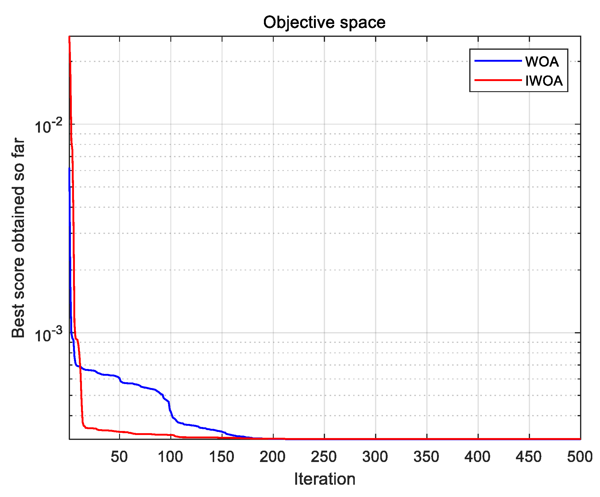
We improve the WOA and design a protection radius with optimal outage probability so that we can search the alternative nodes within the limited protection radius and improve the convergence rate of the traditional WOA.

(3)

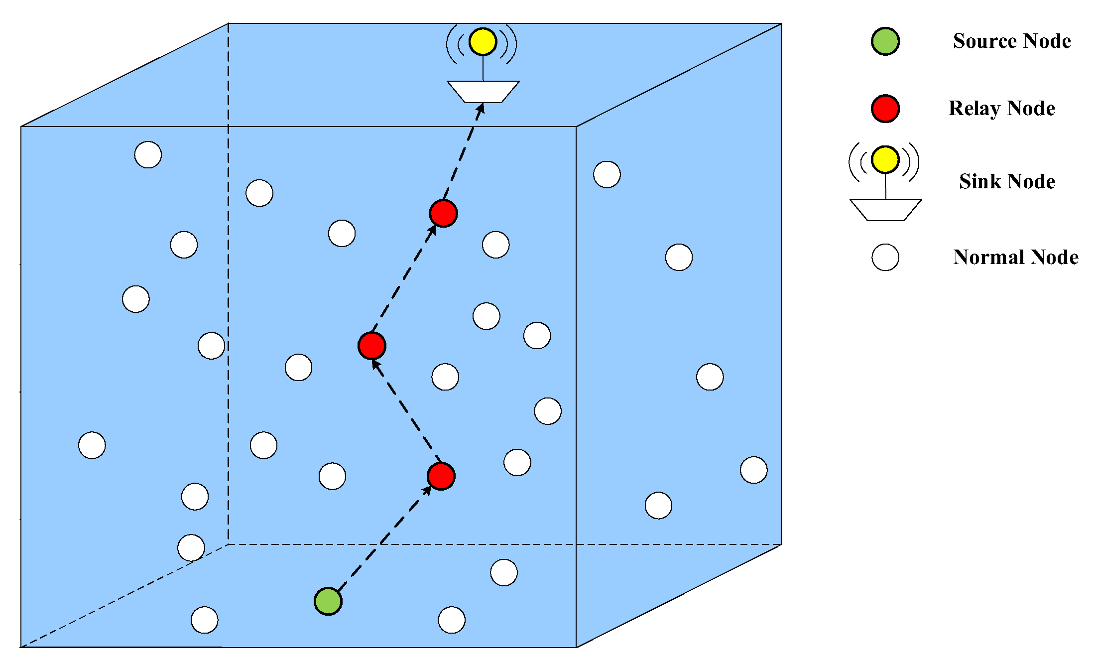
We design the void avoided strategy to suppress the problem of the routing void. In addition, the OCMR can select the optimal relay node in the candidate forwarding set and rapidly rebuild a new route to avoid retransmission when the void occurs.

The remainder of this paper is structured as follows: Section 2 summarizes the related research on UASNs. Section 3 introduces the preliminary WOA and ocean current motion model investigations. In Section 4, the OCMR protocol is described in detail. Section 5 analyses the simulation and results. Finally, the conclusion is given in Section 6.

2. Related Research

The routing protocol has become one of the most important links in UASNs to ensure efficient delivery to the destination node [19]. A well-designed routing protocol is crucial for UASNs to achieve reliable and efficient data transmission. Therefore, scholars from different countries have carried out different studies on the routing protocols of UASNs.

At the beginning of the routing protocol, many studies were based on the geographic locations of sensor nodes with the assumption of their own location information. A routing protocol called vector-based forwarding (VBF) is proposed in [20]. It improves the energy efficiency of the networks with the node location information and creates a virtual routing pipeline. The relay node receives the data transmitted from the sender and then sends them to next receiver within the virtual pipeline. However, nodes falling within this range will be used at a higher frequency than those outside of this range, resulting in uneven energy consumption and a shorter lifetime. However, VBF could not find the relay nodes when the routing void occurred within the pipeline. Hop-by-hop VBF (HH-VBF) was proposed in [21] to address this issue. The pipeline of HH-VBF is different to that of VBF; the routing pipeline is dynamically adjusted according to the location information between the forwarding node and the receiving node in the sparse network, which increases the reliability of data transmission. In [22], an LBL acoustic repeater system was presented, a method based on GNSS. Although the study proved the feasibility of this scheme for obtaining the location of the underwater node, it required four buoys and deduced the underwater node position through three parameters: the surface position, transmission time and depth information of the node. It would eventually cause a higher cumulative error once a parameter error occurred.

In order to avoid using the geographic locations of sensor nodes, a depth-based routing protocol called DBR was proposed in [23]. The packets are greedily delivered from the deep nodes to the shallow nodes. The PDR is improved, and the latency is reduced. However, DBR cannot find the next node as the forwarder when a routing void happens in a sparse network. To address this issue, distance-vector-based opportunistic routing (DVOR) was proposed in [24]. The distance vector is established between the node and destination with the node query mechanism, and the packets are transmitted to the destination node via the shortest path of opportunity.

Energy efficiency in energy-based routing protocols is also an important factor for UASNs because of the energy limitation of underwater sensor nodes. A power-efficient routing protocol (PER) [25] was proposed to reduce the unnecessary power consumption; the overall lifetime of the underwater network will be extended during data forwarding. In addition, a reliable energy-efficient cross-layer routing protocol (RECRP) was proposed in [26]; with a scale-measurement-based Doppler and received-signal-strength indicator, the PDR is increased, and the energy is balanced by a max–min model. However, it is hard to achieve the goal because of the particularity of the underwater environment. Localization-free energy-efficient routing (LFEER) is proposed in [27] to save energy. Although the energy is lowest with an energy-saving mechanism, all nodes will forward the data within the transmission range based on the maximum residual energy. Energy efficiency can still be considered in cluster-based routing protocols. W. R et al. [28] reported a low-energy adaptive clustering hierarchy (LEACH) protocol to reduce the amount of information and minimize energy dissipation with a merging data strategy. The energy load is balanced and benefits from the fair mechanism of cluster head selection. W. Khan et al. [29] proposed a multi-layer cluster-based energy-efficient (MLCEE) protocol to solve the problem of unbalanced transmission via the division of the layer, clustering of the sensor nodes, and forwarding of the data. However, it still has the disadvantages of a delay in data transmission and void hole problems.

Many routing protocols based on data forwarding [30] are used to deliver data to the destination. An evidence-theory-based opportunistic routing (EBOR) [31] protocol was proposed by Z. Jin et al. They chose the best next forwarder according to the residual energy of the node and packet transmission probability. However, this causes high data overheads. There are also some dynamic routing protocols. In [32], the authors propose the self-organized ad hoc mobile (SOAM) routing protocol to solve the routing problem of mobile nodes, but the broadcast packets need to traverse the whole network to achieve connectivity, which leads to higher energy consumption.

Although traditional routing protocols have performed well in UASNs, they are limited by multiple constraints and a high computational complexity [33]. With the advance of artificial intelligence (AI), many intelligent algorithms have been developed for the routing protocol of UASNs, for example, the artificial fish swim algorithm (AFSA), simulated annealing algorithm (SAA), ant colony algorithm (ACA) [34], and Q-learning algorithm. Although these intelligent algorithms can determine the optimal solution through iteration, they still have the shortcoming of falling into the local optimum because of the long search time. QELAR [35] is an energy-efficient and lifetime-aware routing protocol based on Q-learning. In QELAR, the reward function is designed using energy consumption and residual energy to calculate the Q-value; then, the nodes are selected to forward data with a high Q-value. Although QELAR is more energy efficient, it cannot optimize the routing process without depth and latency information. Thus, in [36], Lu et al. propose an energy-efficient depth-based opportunistic routing protocol that performed well in terms of power consumption and PDR. However, the end-to-end delay of the network increased due to the advance detection for the void hole.

The protocols above have their advantages in terms of energy consumption, PDR, network lifetime, etc. However, most of them do not consider the routing void problem caused by the movement of underwater nodes in a real environment. Therefore, we propose OCMR to reduce this problem to avoid data retransmission, reduce the end-to-end delay and improve PDR.

3. Preliminary Investigations

In this section, we mainly explain the reserve knowledge of the whale optimization algorithm (WOA) and ocean current motion model.

3.1. Traditional WOA

The searching process of the WOA includes two phases [37,38,39]: the exploitation phase and the exploration phase. These two phases are explained in the following subsection.

3.1.1. Encircling Prey

Traditionally, humpback whales will surround their prey once they have located them. However, whales are initially unable to determine the optimal location of their prey, so they assume that the current solution is the optimal solution. Subsequently, other search agents update their position to obtain the latest optimal solution iteratively.

The mathematical expression of encircling prey is shown as

$$\overrightarrow{P}=\left|\overrightarrow{C}.\overrightarrow{X^{*}}(t)-\overrightarrow{X}(t)\right|$$

(1)

$$\overrightarrow{X}(t+1)=\overrightarrow{X^{*}}(t)-\overrightarrow{A}\cdot \overrightarrow{P}$$

(2)

where t indicates the number of current iterations, $\overrightarrow{A}$ and $\overrightarrow{C}$ represent the coefficient vectors, $\overrightarrow{X^{*}}(t)$ is the optimal position vector obtained previously, $\overrightarrow{X}(t)$ is the position vector, $\overrightarrow{X}(t+1)$ represents the optimal position vector of next iteration, and $\overrightarrow{P}$ represents the difference in the position vector between two preys. Equation (1) will update $\overrightarrow{X^{*}}(t)$ iteratively when we obtain a better solution.

In Equations (1) and (2), $\overrightarrow{A}$ and $\overrightarrow{C}$ are obtained by

$$\overrightarrow{A}=2\overrightarrow{a}\cdot \overrightarrow{r}-\overrightarrow{a}$$

(3)

$$\overrightarrow{C}=2\cdot \overrightarrow{r}$$

(4)

where $\overrightarrow{a}$ ranges from 2 to 0 and decreases linearly in this interval; $\overrightarrow{r}$ is a random vector in [0, 1].

3.1.2. Bubble-Net Attacking Method (Exploitation Phase)

There are two phases during the exploitation phase: the shrinking encircling mechanism phase and the spiral updating position phase. They are shown as follows:

A. Shrinking encircling mechanism

This behavior is simulated in Equation (3) when we decrease the value of $\overrightarrow{a}$ during this phase. As $\overrightarrow{A}$ ranges from $-a$ to $a$, according to the introduction of $a$, $\overrightarrow{A}$ is at $[-1,1]$.

B. Spiral updating position

Whales search for prey with a spiral encircling approach; this usually occurs during this phase. A spiral equation is expressed as follows:

$$\overrightarrow{X}(t+1)=\overrightarrow{P^{\prime }}\cdot e^{bl}\cdot \cos (2\pi l)+\overrightarrow{X^{*}}(t)$$

(5)

where $\overrightarrow{P^{\prime }}=\left|\overrightarrow{X^{*}}(t)-\overrightarrow{X}(t)\right|$ indicates the distance of the ith whale to the current prey, b is a constant of the logarithmic spiral, and $l$ is a number randomly distributed between −1 and 1.

To update the whale’s optimal position, we assume a 50% chance of choosing between either the shrinking encircling mechanism or the spiral model. The mathematical model of this phase is given as

$$\overrightarrow{X}(t+1)=\{\begin{array}{ll}\overrightarrow{X^{*}}(t)-\overrightarrow{A}\cdot \overrightarrow{P}& if\mathrm{Q}<0.5\\ \overrightarrow{P^{\prime }}\cdot e^{bl}\cdot \cos (2\pi l)+\overrightarrow{X^{*}}(t)& if\mathrm{Q}\ge 0.5,\mathrm{Q}\in [0,1]\end{array}$$

(6)

3.1.3. Search for Prey (Exploration Phase)

In this phase, whales will search for their prey randomly with $\left|\overrightarrow{A}\right|>1$. In this case, the agent will conduct a global search and the optimal position can be updated in a randomly chosen way without reference to the position of the best search agent acquired previously.

The mathematical model is defined as

$$\overrightarrow{P}=\left|\overrightarrow{C}\cdot \overrightarrow{X_{\mathrm{rand}}}-\overrightarrow{X}\right|$$

(7)

$$\overrightarrow{X}(t+1)=\overrightarrow{X_{\mathrm{rand}}}-\overrightarrow{A}\cdot \overrightarrow{P}$$

(8)

where $\overrightarrow{X_{\mathrm{rand}}}$ is a random position vector during the global search.

3.2. Ocean Current Motion Model

It is necessary to estimate the tide and ocean current as these are the main factors affecting the movement of underwater sensor nodes deployed along the seashore.

The movement of nodes in seawater was simulated by a kinematic motion model in [40], which is used on the seashore to handle the specific distribution of nodes. Based on the assumption of the superposition of tidal and remnant flow fields, the Gaussian radial basis function curve is multiplied by different influence factors and tidal components of ocean currents to approximate the movement of sea water. The accurate and real-time seawater motion model is obtained by the selection of the spatial basis function and optimization of model parameters. The model is approximated as

$$\mathrm{y}(v,t)=\{\begin{array}{l}\phi \cdot s\cdot d\cdot {\displaystyle {\sum }_i^N\sin ({\lambda }_i\cdot \mathrm{t})\cdot \psi \cdot \cos ({\eta }_i\cdot \mathrm{t})\cdot \psi }+{\displaystyle {\sum }_i^N\phi \cdot s\cdot \cos (2{\lambda }_i\cdot \mathrm{t})\cdot \psi }+\mu \cdot \psi \\ -s\cdot d\cdot {\displaystyle {\sum }_i^N\cos ({\lambda }_i\cdot \mathrm{t})\cdot \psi \cdot \sin ({\eta }_i\cdot \mathrm{t})\cdot \psi }+p\cdot \psi \end{array}$$

(9)

$$\psi (x,x\prime )=e^{-\frac{\Vert x-x{\prime \Vert }^2}{2{\sigma }^2}}$$

(10)

where N is the tidal number of ocean currents; the time basis functions are denoted by $\sin ({\lambda }_i\cdot \mathrm{t})$, $\sin ({\eta }_i\cdot \mathrm{t})$, $\cos ({\eta }_i\cdot \mathrm{t})$, and $\cos (2{\lambda }_i\cdot \mathrm{t})$; and the frequencies of these functions are $\phi$, $\lambda$, and $\eta$, respectively. $\psi$ is the Gaussian radial basis function; v is the resultant velocity vector of V_y and V_x; and S, d, $\mu$, and p are the impact factors that represent the salinity of the sea water, density, temperature, and pressure, respectively.

As shown in Figure 2 and Figure 3, the motion of sea water shows some semi-periodic and space–time correlation properties. The movement of nodes underwater will change weakly and regularly, so the trajectory of sensor nodes will be predicted by the velocity vector in each direction with limited coverage of the nodes. In the following section of this paper, we will analyze the routing void caused by node drift based on this movement model.

4. OCMR Protocol

This section includes four parts: the protection radius-based construction of the candidate forwarding set, the optimal speed-based relay node selection algorithm, the searching process of the optimal relay node, and the void avoided strategy. These are described in detail below.

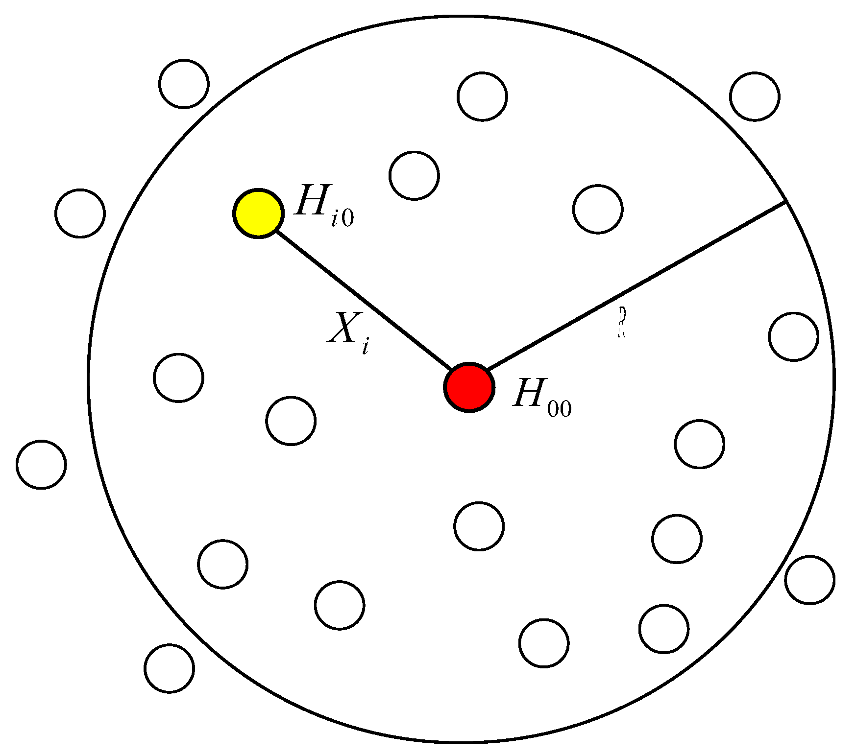
4.1. Protection Radius-Based Construction of the Candidate Forwarding Set

The traditional WOA still has some disadvantages, namely, a low convergence accuracy and rate. Therefore, we need to infer the radius of protection as the selection area of the candidate forwarding set to improve the convergence rate of the traditional WOA.

Data transmission will be affected in a certain area regardless of whether there are too few or too many nodes. If the nodes in the area are few in a sparse network, the point-to-point distance will exceed the maximum communication distance, which will lead to ineffective data transmission. If the nodes in the area are dense, the load of the network will increase, resulting in congestion and data interruption. In order to find an applicable set of forwarding candidates and maintain the nodes of the network in an equilibrium state, we construct the candidate forwarding set with the optimal outage probability as the decision threshold. A suitable WOA search coverage with the optimal outage probability is derived and an appropriate relay node is found within the search coverage. The range is a circle with radius R, namely, the protection radius, in which it can not only select an appropriate relay node to overcome the routing void in the network, but also improve the efficiency of the search.

As shown in Figure 4, a circle is constructed with $H_{00}$ as the center and R as the radius. $H_{i0}$ is the ith node, distributed randomly in the circle. $X_i$ is the distance between $H_{00}$ and $H_{i0}$. We can calculate the communication outage probability among all nodes within the circle as follows:

$$\begin{array}{ll}q(\lambda )& =\mathrm{Pr}(\frac{H_{00}{R}^{-\alpha }}{{\displaystyle \sum _{i\in \Pi }{H}_{i0}{X}_i^{-\alpha }}}<\beta )\\ & =\mathrm{Pr}(H_{00}<\beta R^{\alpha }{I}_{\prod interf})\end{array}$$

(11)

where $\alpha$ is the attenuation coefficient, $\beta$ is the SNR threshold, and $I_{\prod interf}$ is the total interference signal calculated as

$$I_{\prod interf}={\displaystyle \sum _{i\in \Pi }{H}_{i0}{X}_i^{-\alpha }}$$

(12)

As $H_{ij}$ follows an exponential distribution, we obtain

$$f_H(x)=\tau \exp (-\tau x),x\ge 0$$

(13)

Therefore, Equation (11) is converted into

$$q(\lambda )=E[{\displaystyle {\int }_0^{\beta R^{\alpha }{I}_{\Pi }}\tau \exp (-\tau x)dx}]=1-{ℒ}_{I_{\prod interf}}(\tau \beta R^{\alpha })$$

(14)

where ${ℒ}_{I_{\prod interf}}(x)$ is the Laplace transform of $I_{\prod interf}$, which is expressed as

$${ℒ}_{I_{\prod interf}}(s)=\exp (-\alpha \pi \lambda {\displaystyle {\int }_d^{\infty }\frac{s{x}^{-\alpha +1}}{s{x}^{-\alpha }+u}}dx)$$

(15)

Then, we take the iteration from $d$ to $\alpha$. By substituting (15) into (11), Equation (11) can be converted into

$$\begin{array}{ll}q\left(\lambda \right)& =1-\exp \left(-2\pi \lambda {\displaystyle {\int }_d^{\infty }\frac{\tau \beta R^{\alpha }{x}^{-\alpha +1}}{\tau \beta R^{\alpha }{x}^{-\alpha }+\tau }dx}\right)\\ & =1-\exp \left(-2\pi \lambda {\displaystyle {\int }_d^{\infty }\frac{x^{-\alpha +1}}{x^{-\alpha }+{\beta }^{-1}{R}^{-\alpha }}dx}\right)\end{array}$$

(16)

We set $\alpha =4$ due to the Rayleigh fading, and we obtain

$$\begin{array}{ll}{q}_{\alpha =4}\left(\lambda \right)& =1-\exp \left(-2\pi \lambda {\displaystyle {\int }_d^{\infty }\frac{x^{-3}}{x^{-4}+{\beta }^{-1}{R}^{-4}}dx}\right)\\ & =1-\exp [-\pi \lambda {\beta }^{0.5}{R}^{2}arctan({\beta }^{0.5}{R}^2{d}^{-2})]\end{array}$$

(17)

Let $q\left(\lambda \right)=\epsilon$, and $q\left(\lambda \right)$ can be rewritten as

$$q\left(\lambda \right)=1-\exp \{-\lambda \pi {\beta }^{\frac{2}{\alpha }}{R}^2[\frac{1}{\alpha -2}+\ln (\frac{2}{1+d^2{R}^{-2}{\beta }^{-\frac{2}{\alpha }}})]\}$$

(18)

According to the above equation with the optimal outage probability, the optimal protection radius could be calculated as

$$d_{\epsilon }=\sqrt{\frac{\frac{2}{\alpha }{\beta }^{\frac{2}{\alpha }}{R}^2\pi \csc (\frac{2}{\alpha }\pi )}{1-e\ln (1-\epsilon )}}$$

(19)

It can be inferred from the above derivation that the nodes in this circle with radius $d_{\epsilon }$ are the alternative nodes that form the candidate forwarding set.

4.2. Optimal Speed-Based Relay Node Selection Algorithm

The traditional WOA updates the position iteratively based on the position vector, and the optimal node is determined by the fitness value according to different fitness functions. In this paper, we use the velocity vector instead of the node coordinate position to select the relay node.

As is described in Section 3.2, the seawater movement model is used to fit the movement of nodes to reflect the impact of seawater flow on the nodes. We obtain the velocity $V_x$ perpendicular to the coast, velocity $V_y$ along the coast, and velocity function $\mathrm{y}(v,t)$ of time t by Equation (9). The traditional WOA is based on the position vector $\overrightarrow{X}$, and the velocity in the velocity function is also a vector. We can replace $\overrightarrow{X}$ with $\overrightarrow{V}$ to determine the optimal relay node with optimal velocity iteratively in a similar way.

During the initialization phase of the WOA, assuming the number of whales involved in predation is N, the dimension of the searching space is d. The D-dimensional space is represented by

$$\overrightarrow{D}{=(D}^1{,D}^2,\dots {,D}^d)$$

(20)

The position of each whale in the d-dimensional space is given as

$$\overrightarrow{X_i}=(X_i^1,X_i^2,\dots ,X_i^d),i=1,2,\dots ,N$$

(21)

where $\overrightarrow{X_i}$ represents the position of the ith whale in the d-dimensional space. We substitute velocity V of the node into the Equation (21), and we obtain

$$\overrightarrow{V_i}=(V_i^1,V_i^2,\dots ,V_i^d),i=1,2,\dots ,N$$

(22)

where $\overrightarrow{V_i}$ denotes the velocity vector of the ith whale in the d-dimensional space. We assume that the velocity vector $\overrightarrow{V^{*}}$ of the prey is the optimal velocity in the current dimension, and the set of $\overrightarrow{V^{*}}$ is given as

$$\overrightarrow{V^{*}}=(V^{1*},V^{2*},\dots ,V^{d*})$$

(23)

During the encircling prey phase, the iterative model of the velocity vector is shown as

$$\overrightarrow{R^d}=\left|\overrightarrow{C}\cdot \overrightarrow{V^{j*}}(t)-V^j(t)\right|$$

(24)

$$\overrightarrow{V}(t+1)=\overrightarrow{V^{*}}(t)-\overrightarrow{A}\cdot \overrightarrow{R^d}$$

(25)

where t, $\overrightarrow{A}$, and $\overrightarrow{C}$ are described above; $\overrightarrow{V^{*}}(t)$ represents the best velocity vector obtained to date; $\overrightarrow{V}(t+1)$ is the optimal velocity vector of the next iteration; and $\overrightarrow{R^d}$ indicates the subtraction of the velocity vectors between two nodes in the d-dimensional space. We also set $A=2ar-a$, $C=2r$, $a=2-(\frac{2t}{t_{\max }})$, in which $A\in [-1,1]$, as described in Section 3.1.

In the exploitation phase, humpback whales gain on the optimal target using the spiral encircling strategy, which is expressed as

$$\overrightarrow{V}(t+1)=\overrightarrow{V^{*}}(t)+\overrightarrow{r_3\cdot {R^d}^{\prime }}\cdot e^{bl}\cdot \cos (2\pi l)+\sin (V_i^j\left(\mathrm{t}\right))$$

(26)

where $\overrightarrow{{R^d}^{\prime }}=$$\left|\overrightarrow{V^{*}}(t)-\overrightarrow{V}(t)\right|$, and $r_3$ is the balance coefficient in [0, 1]. Similarly, we set the probability of 50% in this phase to obtain the optimal velocity. The model is given as

$$\overrightarrow{V}(t+1)=\{\begin{array}{ll}\overrightarrow{V^{*}}(t)-A\cdot \overrightarrow{R^d}& if\mathrm{Q}<0.5\\ \overrightarrow{V^{*}}(t)+\overrightarrow{{R^d}^{\prime }}\cdot e^{bl}\cdot \cos (2\pi l)+\sin (V_i^j\left(\mathrm{t}\right))& if\mathrm{Q}\ge 0.5\end{array}$$

(27)

When $\left|\overrightarrow{A}\right|\ge 1$ during the search for prey phase, $\overrightarrow{V}(t+1)$ is expressed as

$$\overrightarrow{V}(t+1)=\overrightarrow{V^{*}}(t)-A{\overrightarrow{R^d}}_{predict}+r_1\cdot {\overrightarrow{R^d}}_{best}+r_2\cdot {\overrightarrow{R^d}}_{localbest}$$

(28)

where ${\overrightarrow{R^d}}_{predict}$ denotes the optimal difference value of velocity prediction between two nodes, ${\overrightarrow{R^d}}_{best}$ represents the optimal difference value obtained by iteration between two nodes, ${\overrightarrow{R^d}}_{localbest}$ is the local optimal difference value between two node, and $r_1$ and $r_2$ are balance coefficients in [0, 1].

In order to prove that the improved WOA (IWOA) based on the protection radius has a faster convergence rate, we conduct the simulation comparison between the WOA and IWOA. Please note that the average best-so-far indicates the best solution obtained so far in each iteration over 30 runs. As shown in Figure 5, IWOA obtains the best solution with a smaller number of iterations and IWOA converges faster than the traditional WOA with the protection radius and modified $\overrightarrow{V}(t+1)$ in Equation (28).

We also selected seven classical benchmark functions to compare the avg and std of different functions between IWOA, WOA, PSO and GAS. The basic description of F1–F7 is shown in

Table 1. Basic description of F1–F7.

Function	Num	Range	f min
$F_1(x)={\sum }_{i=1}^n{x}_i^2$	30	[−100,100]	0
$F_2(x)={\sum }_{i=1}^n\left|x_i\right|+{\Pi }_{i=1}^n\left|x_i\right|$	30	[−10,10]	0
$F_3(x)={\sum }_{i=1}^n{([x_i+0.5])}^2$	30	[−100,100]	0
$F_4(x)={\sum }_{i=1}^{n}i{x}_i^4+random[0,1)$	30	[−1.28,1.28]	0
$F_5(x)={\sum }_{i=1}^n-x_i\sin (\sqrt{\left|x_i\right|})$	30	[−500,500]	−418.9829 × 5
$F_6(x)={\sum }_{i=1}^n[x_i^2-10\cos (2\pi x_i)+10]$	30	[−5.12,5.12]	0
$F_7(x)=\frac{\pi }{n}\{10\sin (\pi y_1)+{\sum }_{i=1}^{n-1}{(y_i-1)}^2[1+10{\sin }^2(\pi y_{i+1})]+{(y_n-1)}^2\}+{\sum }_{i=1}^{n}u(x_i,10,100,4)$	30	[−50,50]	0

, and the results of the comparison are shown in

Table 2. Comparison of avg and std of different functions.

Function	IWOA		WOA		PSO		GSA
	Avg	Std	Avg	Std	Avg	Std	Avg	Std
F1	5.3597 × 10−34	4.2268 × 10−18	1.41 × 10−30	4.91 × 10−30	0.000136	0.000202	2.53 × 10−16	9.67 × 10−17
F2	2.0685 × 10−23	2.0727 × 10−23	1.06 × 10−21	2.39 × 10−21	0.042144	0.045421	0.055655	0.194074
F3	1.8898	2.2742	3.116266	0.532429	0.000102	8.28 × 10−5	2.5 × 10−16	1.74 × 10−16
F4	0.00021516	0.009757	0.001425	0.001149	0.122854	0.044957	0.089441	0.04339
F5	−5879.313	600.97165	−5080.76	695.7968	−4841.29	1152.814	−2821.07	493.0375
F6	0	2.98065 × 10−9	0	0	46.70423	11.62938	25.96841	7.470068
F7	0.72669	1.67734	0.339676	0.214864	0.006917	0.026301	1.799617	0.95114

.

4.3. Searching Process of the Optimal Relay Node

In this section, we mainly detail the searching process of the optimal speed-based relay node selection algorithm and protection radius with optimal outage probability.

We first initialize the whale population and velocity, and determine the search coverage with the optimal outage probability using Equation (19). A top-to-bottom view of the surface is shown in Figure 6b.

As shown in Figure 6, (a) is the space diagram of the search area at a certain depth, (b) is the top view of (a). We set the red point A as the center of the circle, and $2d_{\epsilon }$ is the diameter. The diameter splits the circle into two symmetrical parts with a dotted line, forming opposing groups within the search coverage to increase the convergence rate. and represent nodes within opposing groups, and the phase difference between them is $\pi$. indicates the nodes outside the search coverage. Assuming there is a node $v$ in $[l,u]$, then the opposite node $v\prime$ is written as $v\prime =l+u-v$. We suppose $\overrightarrow{v}=(v^1,v^2,\dots ,v^d)$ is a node in the d-dimensional space, where $v^j\in [l^j,u^j],j=1,2,\dots ,d$; the opposite node can be shown as $\overrightarrow{v}\prime =(v^1\prime ,v^2\prime ,\dots ,v^d\prime )$, where $v^j\prime =l^j+u^j-v^j,j=1,2,\dots ,d$. Subsequently, the opposing population is expressed as

$$v_i^j=d_i^j+rand(u_i^j-d_i^j)$$

(29)

$$v_i^{j\prime }=d_i^j+u_i^j-v_i^j$$

(30)

We initialize the population of whales as N and the searching dimension as d, generating the velocity $\overrightarrow{v_i}$ of the ith whale randomly by Equation (29) and the velocity $\overrightarrow{v_i}\prime$ of the ith whale randomly by Equation (30). Whereafter, a fitness function is designed to calculate the fitness value between $\overrightarrow{v_i}$ and $\overrightarrow{v_i}\prime$ iteratively to obtain the whales of N with the optimal fitness value as the initial population. The optimal velocity V is finally obtained iteratively. The probability of a communication outage will increase if the number of nodes is higher or lower. The density of relay nodes in a limited space and selecting an appropriate threshold are most important when selecting the relay nodes in UASNs. The node with a higher residual energy is preferentially selected as the relay node in this density to equalize the energy consumption. Simultaneously, nodes with a relatively low speed should be selected as alternative nodes when the shift in nodes happens. Therefore, the fitness function is defined as Equation (31) based on the above factors.

$$f_{fitness}(V_i)={\omega }_i{f}_{rj}+{\lambda }_{\epsilon }\left(1-\epsilon \right)+\overrightarrow{R^d}\left(V_i\right)\cdot cos\theta (V_i),\theta \in (0,\pi )$$

(31)

$$f_{rj}=\frac{1-E_{\mathrm{rest}}(V_i)}{E_{init}}$$

(32)

where ${\omega }_i$ is the energy coefficient, $f_{rj}$ is an energy parameter, $E_{init}$ represents the initial energy of the node, $E_{\mathrm{rest}}(V_i)$ indicates the residual energy of the node with velocity $V_i$, $\epsilon$ is the outage probability, ${\lambda }_{\epsilon }$ is the node density with the optimal outage probability, $\overrightarrow{R^d}\left(V_i\right)$ represents the relative velocity difference between the node with current velocity $V_i$ and other moving nodes in the search coverage, and $cos\theta$ is the angle between the node with current velocity $V_i$ and other nodes. Finally, the node with the velocity that has the minimum value of the fitness function is the optimal node.

The pseudo-code of the searching process is show in Algorithm 1.

Algorithm 1. Searching process of optimal relay node

– $C(V_i)$: candidate forwarding set based on $d_{\epsilon }$ – $n_{V_i}$: node with velocity V*I – $M\mathrm{axT}$: maximum number of iterations Input: The parameters of nodes including $\alpha$, $V_i$, $\epsilon$, $E_{\mathrm{rest}}(V_i)$, and $E_{init}$ Output: Vi. 1: Initialize the whale population and velocity Vi 2: Calculate the protection radius with optimal outage probability by (19) 3: Generate the opposing population by (29) and (30) 4:  while (t < $M\mathrm{axT}$) 5:   for $n_{V_i}\in C(V_i)$ 6:    Calculate the fitness value to reinitialize population 7:     Update the optimal velocity by (32) 8:      for each search agent 9:       update parameters $\alpha$, A, C, $l$, and Q 10:        if1 (Q < 0.5) 11:         if2 (|A| < 1) 12:          Update the position of the current search agent by Equation (25) 13:         else if2 (|A| ≥ 1) 14:          Update the position of the current search agent by Equation (28) 15:         end if2 16:        else if1 (Q ≥ 0.5) 17:         Update the position of the current search agent by Equation (26) 18:        end if1 19:       end for 20:    end for 21:    for $n_{V_i}\notin C(V_i)$ do 22:   Update $\alpha$ and calculate $d_{\epsilon }$ 23:   end for 24:   Calculate the fitness by Equation (31) 25:   Update V* when a better solution is obtained 26:   t = t + 1 27:  end while 28: Return V*i

4.4. Void Avoided Strategy

If a routing void appears during data transmission, data packets cannot be forwarded effectively, resulting in energy consumption and reduced data transmission efficiency. Therefore, a void avoided strategy is proposed in the OCMR protocol to avoid the routing void. When the relay node shift happens due to ocean currents in the original route, which cause a routing void, a new relay node could be selected in the candidate forwarding set and a new route will be rapidly rebuilt.

The nodes obtain information regarding residual energy, current velocity, etc., from the physical layer on initialization. Then, the relay nodes broadcast the packets to surrounding nodes to obtain information regarding their neighbors. Each node has its own local neighbor table to store the information on neighboring nodes to make routing decisions, for example, packet ID, fitness value, velocity, data, etc. Each node can exchange information with other nodes in the network either as single-hop or multi-hop transfer. The node needs to establish the communication link with the next forwarder via a handshake at first. If the node receives the CTS for the RTS, this indicates a successful handshake between the sender and receiver and the link is reliable. The source node marks the packet ID of each node once the data from this node is received, and preference is given to the relay node in the next data forwarding.

During the construction phase, the set is constructed based on the node as the center and $d_{\epsilon }$ as the radius, after the forwarding link is available for the first time. The transmitting power of the node is adjusted based on $d_{\epsilon }$ in the search coverage to ensure that all nodes can communicate with each other by broadcasting within this protection radius. The interval of broadcasting is $\omega T_{inter}$, where $\omega$ is the time factor, and the $T_{inter}$ is calculated by

$$T_{inter}=\frac{d_{\epsilon }}{V_{\mathit{Acoustic}}}$$

(33)

where $V_{\mathit{Acoustic}}$ represents the propagation velocity of sound in water. The forwarder communicates with all nodes within the communication radius and calculates the fitness value between each node and the forwarder based on the node information. The node with the minimum fitness value can be chosen as the alternative relay node for the forwarder. The fitness value is stored in the routing table of the forwarder and is sent back to the source node during the next data transmission. After receiving the ACK message sent by the forwarder, the source node records the information of the alternate relay node. If a routing void is generated when the forwarder drifts outside the communication radius, caused by the ocean currents, the source node changes the destination node to an alternative relay node to rapidly form a new route.

Taking Figure 7a as an example to illustrate this, an initial communication link is established between source node S and node A after initialization, and A is acquiescently regarded as the optimal forwarder of the next hop during data transmission. After a handshake takes place between S and A, the search coverage with radius $d_{\epsilon }$ and the virtual cone are created. A exchanges information with nodes n1, n2, n3, and n4 in a circle at an interval of $\omega T_{inter}$, and the corresponding fitness value is calculated between n1, n2, n3, and n4, respectively. The fitness value between A and n2 is minimally calculated. So, A saves the information of n2 to its routing table and sends the information back to S via ACK during the next data transmission. No matter which alternative node is chosen, A will always be the forwarder if it is in the search coverage. After a period of time, node B outside the area drifted into the area and became node B′. A exchanges the information with other nodes in the area once again and calculates the corresponding fitness value of each node. The result shows that the fitness value between A and B’ is minimum. Then, A updates the local routing table and replaces n2 with B’ as the optimal alternative relay node. Subsequently, A drifts to A′ outside the circle because of the ocean current motion, and A becomes a routing void. S modifies the forwarding node and chooses B′ as the forwarder to form a new route, and data transmission from S to B′ is achieved.

Nodes will move around with the movement of ocean currents. The node density in the same search coverage and the protection radius will change. The search coverage with a protection radius in a different route also changes as the node density changes, as shown in Figure 7b.

5. Performance Simulation and Analysis

In this section, we evaluate the performance of the OCMR protocol. Firstly, we discuss the parameters of the simulation setting. We compare OCMR with VBF, HH-VBF, and QELAR, which are frequently used in UASNs to demonstrate the performance of the proposed OCMR. There are three performance metrics considered in our simulations: PDR, average end-to-end delay, and average energy consumption. To prove the effectiveness of the proposed protocol, we modify the node density, the node maximum moving velocity, and the node initial energy to analyze three performance metrics.

5.1. Simulation Setting

We use Aqua-sim [41], the built-in underwater acoustic module in NS-2 [42], for simulation to evaluate the performance of OCMR. In the simulation, the sensor nodes are deployed in the region of 800 m × 800 m × 800 m randomly. There is one source node and one destination node in the network scenario, the position of the source node is set to (100, 300, 0), and the position of destination node is set to (400, 400, 800). The node transmission power is 2 W, receiving power is 0.75 W, and idle power is 8 mW. The simulation time is 500 s, the node minimum velocity is 0.2 m/s, the $V_{\mathit{Acoustic}}$ is 1500 m/s underwater, and the transmission range is 100 m. The radius of the routing pipe of the VBF and the HH-VBF is 70 m. The global simulation parameters are shown in

Table 3. Simulation parameters.

Parameters	Values
UASNs deployment space	800 m × 800 m × 800 m
Simulation time	500 s
Communication range	100 m
Transmission power	2 W
Receiving power	0.75 W
Idle power	8 m W
Acoustic speed	1500 m/s
Node minimum velocity	0.2 m/s
Packet size	50 Bytes

.

5.2. Performance Comparison

5.2.1. Influence of the Node Density

In this section, we investigate the influence of the node density to obtain the performance of these protocols. The number of moving nodes ranges from 300 to 1000 in the network, the node moving velocity ranges from 0.2 to 3 m/s, and the initial energy is 100 J. The visualization of simulation results is shown from Figure 8, Figure 9 and Figure 10.

Figure 8 illustrates the comparison of PDR with a different number of nodes. The PDRs of four protocols increase gradually as the number of nodes increases. This is because the probability of a node being selected as a relay node to participate in the data transmission increases with the increasing node density. The OCMR protocol performs better than the VBF, the HH-VBF, and the QELAR in PDR. This is because the candidate forwarding set is formed in the OCMR, and the optimal alternative node will be rapidly selected as the relay node in this set to guarantee the reliability of data transmission when communication is interrupted. The communication link will be reconstructed once the alternative relay node is selected, which reduces unnecessary data collisions and improves the forwarding efficiency, thus increasing the PDR.

Figure 9 presents a comparison of the average end-to-end delay with a different number of nodes. We can see that the performance metrics of four protocols gradually decrease as the number of nodes increases. This is because more neighbors can be chosen as the relay nodes for data forwarding as the number of nodes increases, which reduces the probability of a routing void occurring. Below 600 nodes, the performance of the OCMR protocol is worse than that for the other protocols. This is because more time is needed to extend the protection radius and expand the search coverage to contain more nodes and form a candidate forwarding set in a sparse network. However, when the number of nodes is more than 800, more nodes will be contained in a smaller search coverage, which will reduce the formation time of the candidate forwarding set. However, once the alternative relay node is selected in the forwarding set, the OCMR protocol can suppress the problem of a routing void occurring via the void avoided strategy, which reduces unnecessary data retransmissions.

Figure 10 depicts the comparison of the average energy consumption with a different number of nodes. As the node density increases, the performance metrics of the VBF protocol exhibit fluctuating characteristics because of the limitation imposed by the single routing pipeline; the OCMR, HH-VBF and QELAR protocols tend to balance as node density increase. That is because the total energy consumption grows at the same rate as the number of packets received by the destination node. The metric of the OCMR protocol is better than that of the VBF, HH-VBF, and QELAR protocols. This is because the OCMR algorithm adopts the protection radius to narrow the search coverage, thus improving the forwarding efficiency. However, reliable routing could increase the number of received packets.

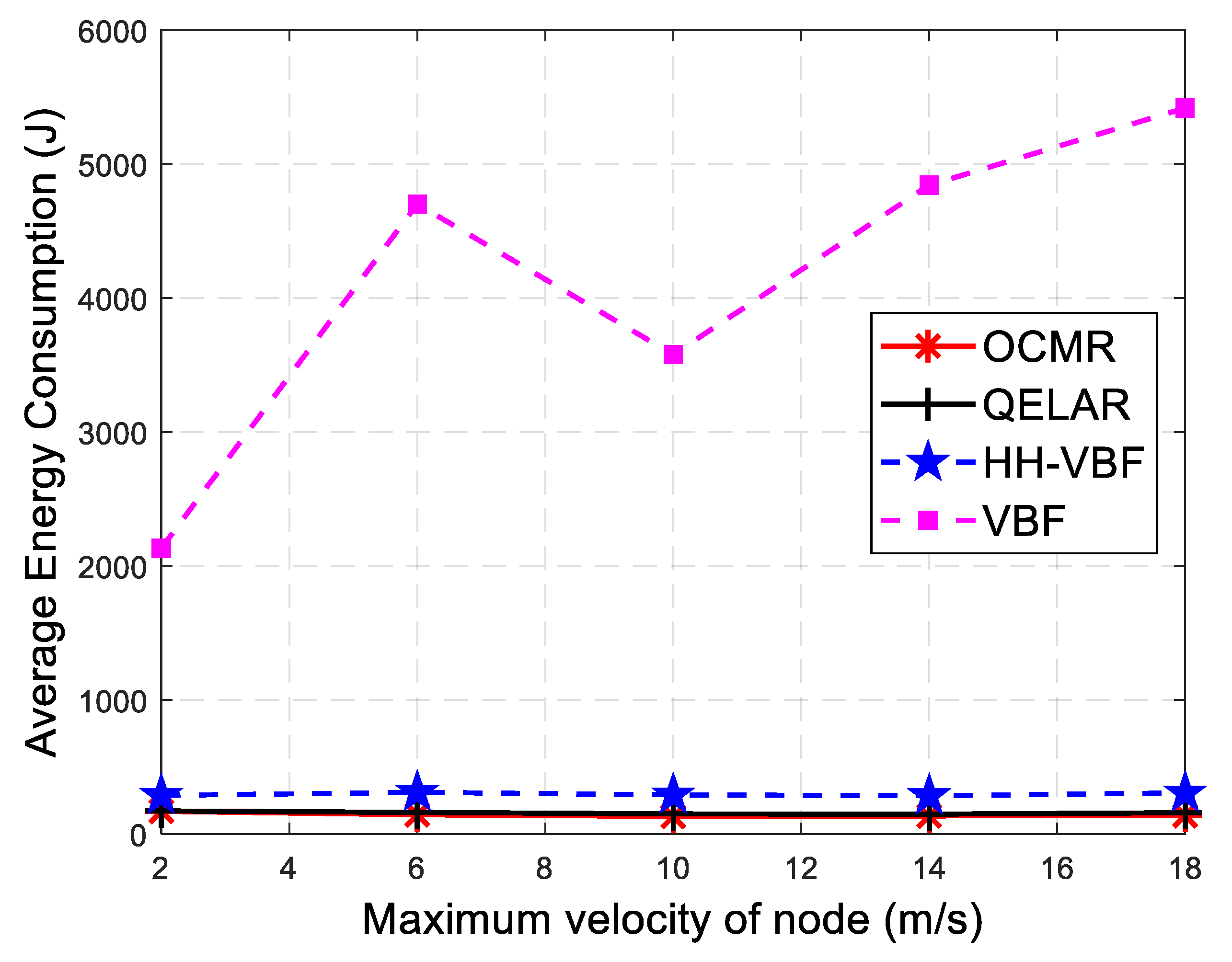
5.2.2. Influence of the Node Maximum Moving Velocity

In this section, we analyze the influence of the maximum node velocity on the performance of these protocols. The number of moving nodes is 800 and the initial energy is 1000 J in this network scenario. The maximum velocity of nodes ranges from 2 to 20 m/s, and the minimum velocity of nodes is 0.2 m/s. A visualization of the simulation results is shown from Figure 11, Figure 12 and Figure 13.

Figure 11 demonstrates the comparison of the PDR with different maximum velocities of the nodes. It can be seen from the figure that the performance of the four protocols is basically stable as the maximum moving velocity of the node increases. This is because they are essentially based on the flooding mechanism. The OCMR protocol performs better than the VBF, HH-VBF, and QELAR protocols because the relative velocity component of node is added to the fitness function, which can better reduce the probability of data loss caused by the change in the moving velocity. However, the candidate forwarding set is formed in the OCMR protocol, which improves the forwarding efficiency and increases the PDR.

Figure 12 represents the comparison of the average end-to-end delay with different maximum node velocities. It is shown in the figure that this performance metric is a little affected by the variation in the maximum moving velocity. This is because the packets of these four protocols are transmitted from the source node to the destination node hop by hop, without an end-to-end communication link. So, they are less affected by the maximum moving velocity of the nodes. The OCMR protocol has the best performance among the four protocols. This is because the relative velocity component of the nodes is added to the fitness function to reduce the effect of the relative moving velocity. However, the OCMR protocol can suppress the problem of a routing void via the voidavoided strategy, which reduces unnecessary data retransmissions.

Figure 13 shows the comparison of the average energy consumption with different maximum node velocities. It can be seen that the performance of the OCMR, HH-VBF, and QELAR protocols are basically stable, but VBF fluctuates with the increase in the maximum moving velocity. This is because the PDR and the average end-to-end delay of the OCMR, HH-VBF and QELAR protocols remain stable with the increase in the maximum moving velocity of the nodes, as shown in Figure 11 and Figure 12. In addition, the number of nodes forwarding the packets is less affected by the maximum moving velocity of the nodes. However, the VBF protocol is greatly affected by the moving velocity because the PDR is restricted by the routing pipeline. The OCMR protocol performed better in terms of the average energy consumption, compared with the other three protocols. This is because the OCMR protocol takes the effect of relative movement velocity into account, and more packets will be received as the nodes move, which reduces the average energy consumption.

5.2.3. Influence of the Node Initial Energy

In this section, we discuss the influence of the node initial energy on the performance of these protocols. The number of moving nodes in the network is set to 1200, the maximum node velocity is 3 m/s, the minimum node velocity is 0.2 m/s, and the initial node energy ranges between 40 J and 160 J. The simulation results can be visualized in Figure 14, Figure 15 and Figure 16.

Figure 14 depicts the comparison of PDR with different initial node energies. It shows that the PDR of the OCMR, QELAR, and HH-VBF protocols first increases and then plateaus with the increase in node initial energy. The VBF protocol performance is basically stable. This is because the nodes can send more packets and use algorithms to find the relay nodes as the initial energy increases. The OCMR and QELAR protocols perform better than other two protocols as the initial energy component of the node is added to the fitness function and the reward function, respectively, which can better balance the energy of the network and improve the forwarding efficiency of the relay node. However, the OCMR protocol performs better than the QELAR protocol, as it profits from the candidate forwarding set based on the protection radius and the voidavoided strategy to increase the efficiency of data forwarding.

Figure 15 represents a comparison of the average end-to-end delay with different initial node energies. It shows that the performance metrics of the four protocols do not change significantly as the node initial energy increases. The performance of the OCMR protocol is the best among them. The reason for this is that the OCMR protocol can suppress the problem of a routing void using the voidavoided strategy, which reduces unnecessary data retransmissions.

Figure 16 illustrates the comparison of the average energy consumption with different node initial energies. It shows that with the increase in the initial energy, the average energy consumption of the QCMR, HH-VBF and QELAR protocols remains stable, and the performance of the VBF protocol experiences a jitter. However, the OCMR protocol is slightly inferior to the QLEAR protocol. This is due to the fact that the OCMR protocol exchanges information with nodes in the search coverage by broadcasting to search for an alternative relay node, which results in additional energy consumption.

6. Conclusions

In this paper, we proposed an oceancurrentmotionmodel-based routing protocol (OCMR) for voidavoided UASNs. This protocol provides an effective method of suppressing the problem of the routing void and the node rapidly selecting the relay node in the candidate forwarding set. In the OCMR protocol, we designed the fitness function with the initial energy, relative velocity, node density, and outage-probability-based modified WOA. To accelerate the convergence of the traditional WOA, we inferred the protectionradius-based optimal outage probability to form the search coverage, which composed the candidate forwarding set. Aiming to solve the problems associated with a routing void, we devised a voidavoided strategy to select an alternate relay node in the alternate forwarding set, which improves the connectivity of the network. Extensive simulation demonstrates that the OCMR protocol outperforms the VBF, HH-VBF, and QELAR protocols in terms of the PDR, average end-to-end delay, and average energy consumption. Additional factors that can be adaptively adjusted will be taken into account in terms of the fitness function in a future study.

References

1. Luo, H.; Wu, K.; Ruby, R.; Liang, Y.; Guo, Z.; Ni, L.M. Softwaredefined architectures and technologies for underwater wireless sensor networks: A survey. IEEE Commun. Surveys Tuts. 2018, 20, 2856–2888. [Google Scholar] [CrossRef]
2. Shahini, A.; Kiani, A.; Ansari, N. Energy efficient resource allocation in EH-enabled CR networks for IoT. IEEE Internet Things J. 2019, 6, 3186–3193. [Google Scholar] [CrossRef]
3. Bujari, A.; Gaggi, O.; Palazzi, C.E.; Ronzani, D. Would current adhoc routing protocols be adequate for the Internet of Vehicles? A comparative study. IEEE Internet Things J. 2018, 5, 3683–3691. [Google Scholar] [CrossRef]
4. Fattah, S.; Gani, A.; Ahmedy, I.; Idris, M.Y.I.; Hashem, I.A.T. A survey on underwater wireless sensor networks: Requirements, taxonomy, recent advances, and open research challenges. Sensors 2020, 20, 5393. [Google Scholar] [CrossRef] [PubMed]
5. Kheirabadi, M.T.; Mohamad, M.M. Greedy routing in underwater acoustic sensor networks: A survey. Int. J. Distrib. Sens. Netw. 2013, 9. [Google Scholar] [CrossRef]
6. Zhang, W.; Han, G.; Wang, X.; Guizani, M.; Fan, K.; Shu, L. A node location algorithm based on node movement prediction in underwater acoustic sensor networks. IEEE Trans. Veh. Technol. 2020, 69, 3166–3178. [Google Scholar] [CrossRef]
7. Khan, Z.A.; Awais, M.; Alghamdi, T.A.; Khalid, A.; Fatima, A.; Akbar, M.; Javaid, N. Region aware proactive routing approaches exploiting energy efficient paths for void hole avoidance in underwater WSNs. IEEE Access 2019, 7, 140703–140722. [Google Scholar] [CrossRef]
8. Sher, A.; Khan, A.; Javaid, N.; Ahmed, S.; Aalsalem, M.; Khan, W. Void hole avoidance for reliable data delivery in IoT enabled underwater wireless sensor networks. Sensors 2018, 18, 3271. [Google Scholar] [CrossRef] [PubMed]
9. Zhang, X.; Yang, P.; Wang, Y.; Shen, W.; Yang, J.; Wang, J.; Ye, K.; Zhou, M.; Sun, H. A Novel Multireceiver SAS RD Processor. IEEE Trans. Geosci. Remote Sens. 2024, 62, 1–11. [Google Scholar] [CrossRef]
10. Zhang, X.; Wu, H.; Sun, H.; Ying, W. Multireceiver SAS imagery based on monostatic conversion. IEEE J. Sel. Top. Appl. Earth Obs. Remote Sens. 2021, 14, 10835–10853. [Google Scholar] [CrossRef]
11. Yang, P. An imaging algorithm for high-resolution imaging sonar system. Multimed. Tools Appl. 2023, 83, 31957–31973. [Google Scholar] [CrossRef]
12. Zhang, X. An efficient method for the simulation of multireceiver SAS raw signal. Multimed. Tools Appl. 2023, 1–18. [Google Scholar] [CrossRef]
13. Tuna, G.; Gungor, V.C. A survey on deployment techniques, localization algorithms, and research challenges for underwater acoustic sensor networks. Int. J. Commun. Syst. 2017, 30, e3350. [Google Scholar] [CrossRef]
14. Gong, Z.; Li, C.; Su, R. Fundamental Limits of Doppler Shift-Based, ToA-Based, and TDoA-Based Underwater Localization. IEEE/CAA J. Autom. Sin. 2023, 10, 1637–1639. [Google Scholar] [CrossRef]
15. Zhang, B.; Zhu, J.; Wu, Y.; Zhang, W.; Zhu, M. Underwater localization using differential doppler scale and TDOA measurements with clock imperfection. Wirel. Commun. Mob. Comput. 2022, 2022, 6597132. [Google Scholar] [CrossRef]
16. Mirjalili, S.; Lewis, A. The whale optimization algorithm. Adv. Eng. Softw. 2016, 95, 51–67. [Google Scholar] [CrossRef]
17. Mirjalili, S. The ant lion optimizer. Adv. Eng. Softw. 2015, 83, 80–98. [Google Scholar] [CrossRef]
18. Mirjalili, S.; Mirjalili, S.M.; Lewis, A. Grey wolf optimizer. Adv. Eng. Softw. 2014, 69, 46–61. [Google Scholar] [CrossRef]
19. Jiang, J.; Han, G.; Lin, C. A survey on opportunistic routing protocols in the Internet of Underwater Things. Comput. Netw. 2023, 225, 109658. [Google Scholar] [CrossRef]
20. Xie, P.; Cui, J.-H.; Lao, L. VBF: Vector-based forwarding proto-col for underwater sensor networks. In NETWORKING 2006. Networking Technologies, Services, and Protocols; Performance of Computer and Communication Networks; Mobile and Wireless Communications Systems; Lecture Notes in Computer Science; Springer: Berlin/Heidelberg, Germany, 2006; Volume 3976, pp. 1216–1221. [Google Scholar]
21. Nicolaou, N.; See, A.; Peng, X.; Jun-Hong, C.; Maggiorini, D. Improving the robustness of location-based routing for underwater sensor networks. In Proceedings of the OCEANS 2007—Europe, Aberdeen, UK, 18–21 June 2007; pp. 1–6. [Google Scholar]
22. Otero, P.; Hernández-Romero, Á.; Luque-Nieto, M.Á.; Ariza, A. Underwater Positioning System Based on Drifting Buoys and Acoustic Modems. J. Mar. Sci. Eng. 2023, 11, 682. [Google Scholar] [CrossRef]
23. Yan, H.; Shi, Z.J.; Cui, J.H. DBR: Depth-based routing for underwater sensor networks. In NETWORKING 2008 Ad Hoc and Sensor Networks, Wireless Networks, Next Generation Internet; Springer: Berlin/Heidelberg, Germany, 2008; pp. 72–86. [Google Scholar]
24. Guan, Q.; Ji, F.; Liu, Y.; Yu, H.; Chen, W. Distance-vector based opportunistic routing for underwater acoustic sensor networks. IEEE Internet Things J. 2019, 6, 3831–3839. [Google Scholar] [CrossRef]
25. Huang, C.-J.; Wang, Y.-W.; Liao, H.-H.; Lin, C.-F.; Hu, K.-W.; Chang, T.-Y. A power-efficient routing protocol for underwater wireless sensor networks. Appl. Soft Comput. J. 2011, 11, 2348–2355. [Google Scholar] [CrossRef]
26. Liu, J.; Yu, M.; Wang, X.; Liu, Y.; Wei, X. RECRP: A reliable energy-efficient cross-layer routing protocol in UWSNs. In Proceedings of the 2018 OCEANS—MTS/IEEE Kobe Techno-Oceans (OTO), Kobe, Japan, 28–31 May 2018; pp. 1–4. [Google Scholar]
27. Shah, S.; Khan, A.; Ali, I.; Ko, K.-M.; Mahmood, H. Localization free energy efficient and cooperative routing protocols for underwater wireless sensor networks. Symmetry 2018, 10, 498. [Google Scholar] [CrossRef]
28. Heinzelman, W.R.; Chandrakasan, A.; Balakrishnan, H. Energyefficient communication protocol for wireless microsensor networks. In Proceedings of the 33rd Annual Hawaii International Conference on System Sciences, Maui, HI, USA, 7 January 2000; p. 223. [Google Scholar]
29. Khan, W.; Wang, H.; Anwar, M.S.; Ayaz, M.; Ahmad, S.; Ullah, I. A multi-layer cluster based energy efficient routing scheme for UWSNs. IEEE Access 2019, 7, 77398–77410. [Google Scholar] [CrossRef]
30. Jiang, S.; Member, S. On reliable data transfer in underwater acoustic networks: A survey from networking perspective. IEEE Commun. Surv. Tuts. 2018, 20, 1036–1055. [Google Scholar] [CrossRef]
31. Jin, Z.; Ji, Z.; Su, Y. An evidence theory based opportunistic routing protocol for underwater acoustic sensor networks. IEEE Access 2018, 6, 71038–71047. [Google Scholar] [CrossRef]
32. Hyder, W.; Pabani, J.K.; Luque-Nieto, M.Á.; Laghari, A.A.; Otero, P. Self-Organized Ad Hoc Mobile (SOAM) Underwater Sensor Networks. IEEE Sens. J. 2022, 23, 1635–1644. [Google Scholar] [CrossRef]
33. Li, N.; Martínez, J.-F.; Chaus, J.M.M.; Eckert, M. A survey on underwater acoustic sensor network routing protocols. Sensors 2016, 16, 414. [Google Scholar] [CrossRef]
34. Zhang, J.; Liu, H.; Tong, S.; Wang, L. The improvement of ant colony al-gorithm and its application to tsp problem. In Proceedings of the 2009 5th International Conference on Wireless Communications, Networking and Mobile Computing, Beijing, China, 24–26 September 2009; pp. 1–4. [Google Scholar]
35. Hu, T.; Fei, Y. QELAR: A machine-learning-based adaptive routing protocol for energy-efficient and lifetime-extended underwater sensor networks. IEEE Trans. Mob. Comput. 2010, 9, 796–809. [Google Scholar] [CrossRef]
36. Lu, Y.; He, R.; Chen, X.; Lin, B.; Yu, C. Energy-efficient depth-based opportunistic routing with Q-learning for underwater wireless sensor networks. Sensors 2020, 20, 1025. [Google Scholar] [CrossRef]
37. Olorunda, O.; Engelbrecht, A.P. Measuring exploration/exploitation in particle swarms using swarm diversity. In Proceedings of the 2008 IEEE Congress on Evolutionary Computation, CEC (IEEE World Congress on Computational Intelligence), Hong Kong, China, 1–6 June 2008; pp. 1128–1134. [Google Scholar]
38. Alba, E.; Dorronsoro, B. The exploration/exploitation tradeoffin dynamic cellular genetic algorithms. IEEE Trans. Evol. Comput. 2005, 9, 126–142. [Google Scholar] [CrossRef]
39. Lin, L.; Gen, M. Auto-tuning strategy for evolutionary algorithms: Balancing between exploration and exploitation. Soft Comput. 2009, 13, 157–168. [Google Scholar] [CrossRef]
40. SBeerens, P.; Ridderinkhof, H.; Zimmerman, J. An Analytical Study of Chaotic Stirring in Tidal Areas. Chaos Solitons Fractals 1994, 4, 1011–1029. [Google Scholar] [CrossRef]
41. Xie, P.; Zhou, Z.; Peng, Z.; Yan, H.; Hu, T.; Cui, J.-H.; Shi, Z.; Fei, Y.; Zhou, S. Aqua-Sim: An NS-2 based simulator for underwater sensor networks. In Proceedings of the OCEANS 2009, Biloxi, MS, USA, 26–29 October 2009; pp. 1–7. [Google Scholar]
42. Issariyakul, T.; Hossain, E. Introduction to Network Simulator 2 (NS2); Springer: Boston, MA, USA, 2012. [Google Scholar]
Figure 1. Routing diagram of UASNs.
Jmse 12 00537 g001
Figure 2. Velocity perpendicular to the coast.
Jmse 12 00537 g002
Figure 3. Velocity along the coast.
Jmse 12 00537 g003
Figure 4. Protection radius diagram.
Jmse 12 00537 g004
Figure 5. Comparison of convergence rates of WOA and IWOA.
Jmse 12 00537 g005
Figure 6. (a) spave diagram of search area. (b) planform of search area.
Jmse 12 00537 g006
Figure 7. (a) Routing strategy diagram (single-hop process). (b) Routing strategy diagram (multi-hop process).
Jmse 12 00537 g007
Figure 8. Comparison of PDR with different numbers of nodes.
Jmse 12 00537 g008
Figure 9. Comparison of average end-to-end delay with a different number of nodes.
Jmse 12 00537 g009
Figure 10. Comparison of average energy consumption with different number of nodes.
Jmse 12 00537 g010
Figure 11. Comparison of PDR with different maximum node velocities.
Jmse 12 00537 g011
Figure 12. Comparison of average end-to-end delay with different maximum node velocities.
Jmse 12 00537 g012
Figure 13. Comparison of average energy consumption with different maximum node velocities.
Jmse 12 00537 g013
Figure 14. Comparison of PDR with different initial node energies.
Jmse 12 00537 g014
Figure 15. Comparison of average end-to-end delay with different node initial energies.
Jmse 12 00537 g015
Figure 16. Comparison of average energy consumption with different node initial energies.
Jmse 12 00537 g016