An Application of 3D Cross-Well Elastic Reverse Time Migration Imaging Based on the Multi-Wave and Multi-Component Technique in Coastal Engineering Exploration

Abstract

Precise surveys are indispensable in coastal engineering projects. The extensive presence of sand in the coastal area leads to significant attenuation of seismic waves within unsaturated loose sediments. As a result, it becomes challenging for seismic waves to penetrate the weathered zone and reach the desired depth with significant amount of energy. In this study, the application of three-dimensional (3D) cross-well elastic reverse time migration (RTM) imaging based on multi-wave and multi-component techniques in coastal engineering exploration is explored. Accurate decomposition of vector compressional (P) and shear (S) waves is achieved through two wavefield decoupling algorithms without any amplitude and phase distortion. Additionally, compressional wave pressure components are obtained, which facilitates subsequent independent imaging. This study discusses and analyzes the imaging results of four imaging strategies under cross-correlation imaging conditions in RTM imaging. The analysis leads to the conclusion that scalarizing vector wavefields imaging yields superior imaging of P- and S-waves. Furthermore, the imaging results obtained through this approach are of great physical significance. In order to validate the efficacy of this method in 3D geological structure imaging in coastal areas, RTM imaging experiments were performed on two representative models. The results indicate that the proposed 3D elastic wave imaging method effectively generates accurate 3D cross-well imaging of P- and S-waves. This method utilizes the multi-wave and multi-component elastic wave RTM imaging technique to effectively leverage the Earth’s elastic medium without increasing costs. It provides valuable information about the distribution of subsurface rock layers, interfaces, and other structures in coastal engineering projects. Importantly, this can be achieved without resorting to extensive excavation or drilling operations. This method addresses the limitations of current cross-well imaging techniques, thereby providing abundant and accurate geological and geophysical information for the analysis and interpretation of 3D geological structures in coastal engineering projects. It has important theoretical and practical significance in real-world production, as well as for the study of geological structures in coastal engineering.

1. Introduction

During coastal engineering projects, extensive surveys and investigations are crucial for gathering information on geological structures, sediment distribution, and soil properties in coastal areas. These investigations involve analyses by drilling, sampling, and geophysical exploration to evaluate the geological formations, soil types, lithology, and groundwater levels [1,2,3]. Among the numerous geophysical exploration methods, seismic exploration is widely employed due to its ability to provide superior subsurface resolution [4]. However, the extensive presence of sand in the coastal area leads to a significant attenuation of seismic waves within unsaturated loose sediments. Surface seismic methods are highly susceptible to variations in near-surface conditions and encountering difficulties in transmitting a significant amount of energy through the weathered zone to reach the targeted depths [5,6,7]. Compared to surface seismic reflection or refraction surveys, cross-well seismic acquisition methods emerge as an optimal choice for effectively targeting specific coastal areas [8,9].

Cross-well seismic can be applied to various aspects of oil and gas exploration, including detailed imaging of structures and precise characterization of reservoirs [10,11,12]. Furthermore, cross-well seismic has also been rapidly developed in the field of engineering [13,14] and has been applied in diverse areas, such as geological engineering [15,16,17], hydrogeological surveys [18,19,20], and quality inspections in civil engineering projects [21,22,23]. Currently, most cross-well seismic studies focus on two-dimensional (2D) tomographic imaging between adjacent wells [24,25]. It requires data collection and travel-time inversion between two wells to acquire subsurface structural profiles. Nevertheless, this imaging approach has certain limitations. For example, in 2D computed tomography (CT) imaging, only adjacent wells can be imaged, and information from multiple wells distributed in 3D space cannot be effectively utilized [26]. As a result, the utilization rate of spatial well locations remain relatively low. Furthermore, the 2D cross-well CT imaging technique can only provide information on the geological structure of the profile between the two wells, failing to capture the lateral structure information of the profile [27]. As a result, the imaging provides poor lateral continuity, hindering the evaluation of 3D geological structures.

Additionally, there are issues associated with imaging steep-dip interfaces (interfaces with dip angles exceeding 45°) [28]. In recent years, the rapidly developing RTM method follows the full-wave wave equation during wavefield extrapolation and is not limited by angles [29,30,31]. Among various pre-stack migration methods, RTM is considered the most accurate imaging technique. However, current studies on cross-well RTM imaging are limited to 2D space or 3D P-waves RTMs [32,33]. With the advancement of seismic exploration technology, the challenges have become increasingly complex. Conventional compressional wave exploration can no longer satisfy the needs of engineering projects [34]. Improvements need to be made in two key aspects: First, it is necessary to image areas with weak compressional wave reflection energy or no compressional wave reflection signals to provide reliable structural imaging information. Second, it is necessary to provide imaging information for elastic multi-wave analysis, thus establishing a reliable foundation for subsequent elastic wave amplitude analysis and rock physics parameter inversion. Conventional seismic exploration techniques commonly employ compressional wave sources. To address the limitations of compressional wave reflection energy, the shear waves generated through compressional wave conversion need to be imaged [35,36]. This approach aims to fully utilize the Earth’s elastic media to construct comprehensive imaging information of subsurface structures without increasing costs. Simultaneously, the imaging results must include multi-wave imaging results for subsequent amplitude variation with angle (AVA) analysis and the inversion of rock physics parameters [37,38]. Compared with the conventional compressional wave exploration techniques, the theoretical assumptions of multi-wave and multi-component seismic exploration technology are more consistent with the actual characteristics of subsurface media, offering significant advantages in addressing practical challenges.

To effectively address the above issues, it is essential to fully utilize the distinctive features of multi-wave and multi-component seismic data acquired between wells. Therefore, this paper investigates the application of 3D cross-well elastic wavefield RTM imaging in coastal engineering exploration based on multi-wave and multi-component data. By applying multi-wave and multi-component elastic wave RTM imaging techniques, precise 3D geological structures between wells can be obtained, laying the foundation for subsequent lithological analysis and inversion. This approach addresses the limitations of current cross-well imaging techniques, thus providing rich geological and geophysical information for analyzing and interpreting 3D geological structures in coastal regions. It has important theoretical and practical significance in actual production, as well as for the investigation of geological structures in coastal engineering.

2. Methodology

To study the application of 3D cross-well seismic exploration in coastal engineering, it is essential to first conduct research on the numerical simulation of elastic waves. Numerical simulations encompass the simulation of the propagation characteristics of elastic waves in various media through mathematical methods based on the known physical parameters of the detection model, combined with elastic wave propagation theory [39]. Numerical simulations can be divided into three categories: wave equation numerical methods, integral methods, and ray tracing methods. Among these, wave equation numerical methods primarily include the finite difference method (FDM) [40], pseudo spectral method (PSM) [41], finite element method (FEM) [42], spectral element method (SEM) [43], and boundary element method (BEM) [44]. FDM is extensively employed in numerical simulations of elastic waves due to its advantageous features, including fast computation speed and high accuracy.

In this section, we begin by discussing the 3D elastic wave equations of motion and grid discretization in cylindrical coordinates. Then, we utilize two different methods for elastic wave decomposition. Following this, we introduce the principles of RTM imaging and provide detailed explanations of four different cross-correlation imaging conditions. Lastly, we propose the Poynting vector and Laplace filtering to attenuate RTM imaging artifacts.

2.1. 3D Elastic Wave Equations of Motion and Grid Discretization

The basic laws governing the propagation of elastic waves are described by the wave equation of elastic waves. Based on the equations of motion, Cauchy equations, and physical equations in a three-dimensional Cartesian coordinate system, the first-order velocity-stress equation in an isotropic medium in cylindrical coordinates can be expressed as follows [45]:

$$\{\begin{array}{c}\rho \frac{\partial v_x}{\partial t}=\frac{\partial {\tau }_{xx}}{\partial x}+\frac{\partial {\tau }_{xy}}{\partial y}+\frac{\partial {\tau }_{xz}}{\partial z}+f_x\\ \rho \frac{\partial v_y}{\partial t}=\frac{\partial {\tau }_{xy}}{\partial x}+\frac{\partial {\tau }_{yy}}{\partial y}+\frac{\partial {\tau }_{yz}}{\partial z}+f_y\\ \rho \frac{\partial v_z}{\partial t}=\frac{\partial {\tau }_{xz}}{\partial x}+\frac{\partial {\tau }_{yz}}{\partial y}+\frac{\partial {\tau }_{zz}}{\partial z}+f_z\end{array}$$

(1)

$$\{\begin{array}{l}\frac{\partial {\tau }_{xx}}{\partial t}=\left(\lambda +2\mu \right)\frac{\partial v_x}{\partial x}+\lambda \left(\frac{\partial v_y}{\partial y}+\frac{\partial v_z}{\partial z}\right)+g_{xx}\\ \frac{\partial {\tau }_{yy}}{\partial t}=\left(\lambda +2\mu \right)\frac{\partial v_y}{\partial y}+\lambda \left(\frac{\partial v_x}{\partial x}+\frac{\partial v_z}{\partial z}\right)+g_{yy}\\ \frac{\partial {\tau }_{zz}}{\partial t}=\left(\lambda +2\mu \right)\frac{\partial v_z}{\partial z}+\lambda \left(\frac{\partial v_y}{\partial y}+\frac{\partial v_x}{\partial x}\right)+g_{zz}\\ \frac{\partial {\tau }_{xy}}{\partial t}=\mu (\frac{\partial v_x}{\partial y}+\frac{\partial v_y}{\partial x})+g_{xy}\\ \frac{\partial {\tau }_{yz}}{\partial t}=\mu (\frac{\partial v_y}{\partial z}+\frac{\partial v_z}{\partial y})+g_{xz}\\ \frac{\partial {\tau }_{xz}}{\partial t}=\mu (\frac{\partial v_z}{\partial x}+\frac{\partial v_x}{\partial z})+g_{yz}\end{array}$$

(2)

where $v={\left[v_x,v_y,v_z\right]}^T$ denotes the velocity; $\tau ={\left[{\tau }_{xx},{\tau }_{yy},{\tau }_{zz},{\tau }_{xy},{\tau }_{yz},{\tau }_{xz}\right]}^T$ denotes the stress vectors; $f={\left[f_x,f_y,f_z\right]}^T$ represents the point force source; $g={\left[g_{xx},g_{yy},g_{zz},g_{xy},,g_{xz},g_{yz}\right]}^T$ represents the coupling; $\rho$ is the density; $\lambda$ and $\mu$ refer to the Lamé constants.

2.2. Elastic Wave Decomposition

For elastic wave RTM, the key to obtaining multi-wave and multi-component migration results is the decoupling of P- and S-waves. The elastic wavefields are separated during the reconstruction of the source and receiver wavefields to obtain pure P-wave and S-wave wavefields [46]. The following two methods are employed in this study.

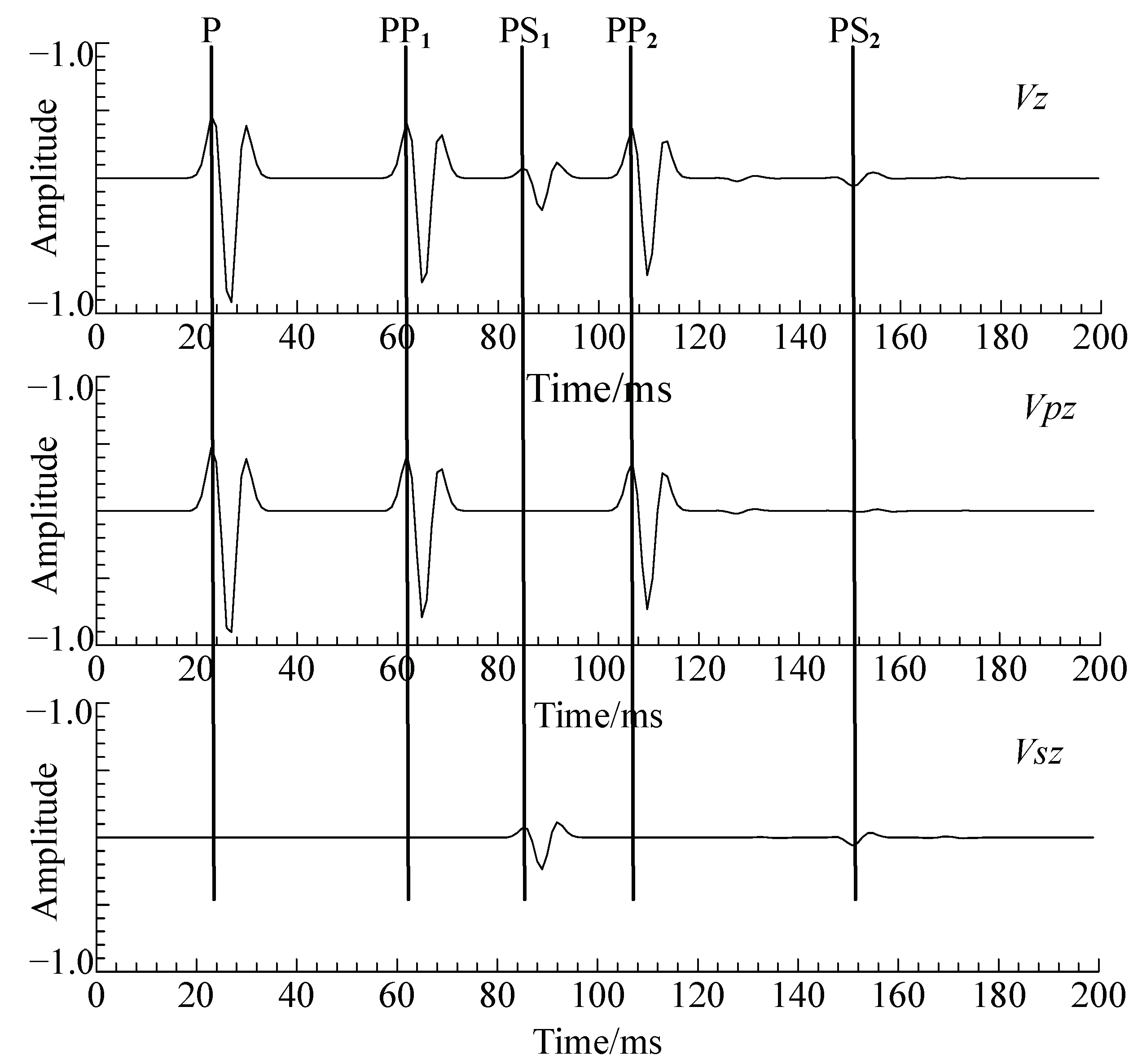
2.2.1. Wave Equation Decoupling Method

Based on the homogeneous isotropic media and the first-order velocity-stress equations, the velocities of separated P- and S-waves in 3D space can be expressed as follows [47]:

$$\{\begin{array}{l}\begin{array}{c}\begin{array}{c}{v}_x=v_{px}+v_{sx}\\ v_y=v_{py}+v_{sy}\end{array}\\ v_z=v_{pz}+v_{sz}\end{array}\\ \frac{\partial v_{px}}{\partial t}=\frac{\lambda +2\mu }{\rho \left(3\lambda +2\mu \right)}\left(\frac{{\sigma }_{xx}}{\partial x}+\frac{{\sigma }_{yy}}{\partial x}+\frac{{\sigma }_{zz}}{\partial x}\right)\\ \frac{\partial v_{py}}{\partial t}=\frac{\lambda +2\mu }{\rho \left(3\lambda +2\mu \right)}\left(\frac{{\sigma }_{xx}}{\partial y}+\frac{{\sigma }_{yy}}{\partial y}+\frac{{\sigma }_{zz}}{\partial y}\right)\\ \frac{\partial v_{pz}}{\partial t}=\frac{\lambda +2\mu }{\rho \left(3\lambda +2\mu \right)}\left(\frac{{\sigma }_{xx}}{\partial y}+\frac{{\sigma }_{yy}}{\partial y}+\frac{{\sigma }_{zz}}{\partial y}\right)\\ \frac{\partial v_{sx}}{\partial t}=\frac{1}{\rho }\left(\frac{{\sigma }_{xy}}{\partial y}+\frac{{\sigma }_{xz}}{\partial z}\right)+\frac{1}{\rho \left(3\lambda +2\mu \right)}\left[\left(\lambda +2\mu \right)\left(\frac{{\sigma }_{yy}}{\partial x}+\frac{{\sigma }_{zz}}{\partial x}\right)-2\lambda \frac{{\sigma }_{xx}}{\partial x}\right]\\ \frac{\partial v_{sy}}{\partial t}=\frac{1}{\rho }\left(\frac{{\sigma }_{xy}}{\partial x}+\frac{{\sigma }_{yz}}{\partial z}\right)+\frac{1}{\rho \left(3\lambda +2\mu \right)}\left[\left(\lambda +2\mu \right)\left(\frac{{\sigma }_{xx}}{\partial y}+\frac{{\sigma }_{zz}}{\partial y}\right)-2\lambda \frac{{\sigma }_{yy}}{\partial y}\right]\\ \frac{\partial v_{sz}}{\partial t}=\frac{1}{\rho }\left(\frac{{\sigma }_{xz}}{\partial x}+\frac{{\sigma }_{yz}}{\partial z}\right)+\frac{1}{\rho \left(3\lambda +2\mu \right)}\left[\left(\lambda +2\mu \right)\left(\frac{{\sigma }_{xx}}{\partial z}+\frac{{\sigma }_{yy}}{\partial z}\right)-2\lambda \frac{{\sigma }_{zz}}{\partial z}\right]\end{array}$$

(3)

In Equation (3), v_px and v_sx represent the P- and S-wave components in the x-direction, respectively. Similarly, v_py and v_sy represent the P- and S-wave components in the y-direction, and v_pz and v_sz represent the P- and S-wave components in the z-direction, respectively. By solving Equation (3), the wavefields of pure P- and S-waves can be obtained. With this method, the amplitude and phase information of the P- and S-waves can be better retained.

2.2.2. Auxiliary Variables Method

In addition to the six velocity component equations incorporated in the equation for conventional elastic wave, the method of auxiliary variables introduces an additional component to achieve the vector decomposition of P- and S-waves, which is the compressional wave pressure component equation [48,49]. The expression of this equation is as follows:

$$\{\begin{array}{l}\frac{\partial {\tau }_p}{\partial t}=\left(\lambda +2\mu \right)\left(\frac{\partial v_x}{\partial x}+\frac{\partial v_y}{\partial y}+\frac{\partial v_z}{\partial z}\right)\\ \frac{\partial v_{px}}{\partial t}=\frac{1}{\rho }\frac{\partial {\tau }_p}{\partial x} v_{sx}=v_x-v_{px}\\ \frac{\partial v_{py}}{\partial t}=\frac{1}{\rho }\frac{\partial {\tau }_p}{\partial y} v_{sy}=v_y-v_{py}\\ \frac{\partial v_{pz}}{\partial t}=\frac{1}{\rho }\frac{\partial {\tau }_p}{\partial z} v_{sz}=v_z-v_{pz}\end{array}$$

(4)

In the method of auxiliary variables, the introduction of the τ_p component allows for additional wavefield information to be obtained. The τ_p component is analogous to the acoustic pressure component in the acoustic wave equation. In the context of elastic waves, it represents the pressure component of the P-wave [50].

2.3. Cross-Correlation Imaging Condition

The RTM algorithm, with its significant impact on imaging accuracy, relies heavily on the imaging condition [51,52]. Different imaging conditions employed in the imaging process can lead to different imaging results. The following sections introduce four cross-correlation imaging conditions used in elastic RTM.

2.3.1. Imaging by Vector Velocity Fields

In conventional elastic RTM imaging, the complete wavefield is employed for the imaging process. For multi-component seismic data, the velocity wavefields of the source (v^S(x,t)) and the receiver (v^R(x,t)) in the subsurface at each position x can be obtained through forward modeling and wavefield extrapolation. The imaging condition utilizing the three-component velocity wavefields can be expressed as follows:

$$I_{ij}\left(\mathbf{x}\right)={\displaystyle {\int }_0^{T_{\max }}{v}_i^S\left(\mathbf{x},t\right)\cdot v_j^R\left(\mathbf{x},t\right)}dt$$

(5)

where S and R represent the velocity wavefields of the source and receiver, respectively; i and j correspond to the three Cartesian components: x, y, and z; and I_ij represents the imaging structure generated by cross-correlating the i-component of the source wavefield with the j-component of the receiver wavefield. T_max is the maximum time of the seismic records. This method can introduce crosstalk between P- and S-waves in both the source wavefield and the receiver wavefield.

2.3.2. Imaging by Scalar and Vector Potentials

Under the elastic RTM imaging condition, the second imaging method is implemented. It utilizes the Helmholtz decomposition during the extrapolation of the wavefield, effectively separating the source wavefield and receiver wavefield into pure P- and S-wave wavefields. The expression of the imaging condition is as follows:

$$I_{ij}\left(\mathbf{x}\right)={\displaystyle {\int }_0^{T_{\max }}{m}_i^S\left(\mathbf{x},t\right)\cdot m_j^R\left(\mathbf{x},t\right)}dt$$

(6)

where S and R represent the velocity wavefields of the source and receiver, respectively; i and j correspond to different wave modes, specifically the P- and S-waves. T_max is the maximum time of the seismic records. This method modifies the phase and amplitude characteristics of the original wavefield when employing the Helmholtz decomposition.

2.3.3. Imaging by Pure Vector P- and S-Waves

Using the separation method described in Equation (3), pure P- and S-wave wavefields in various directions can be obtained. Afterward, during the process of wavefield extrapolation, these separated wavefields are utilized as boundary conditions. The imaging results of the P- and S-wave vector components can be acquired through correlating the source wavefield with the receiver wavefield. Figure 1 illustrates the imaging process for this method.

The following expression represents the imaging condition for elastic wave RTM using vector P- and S-wave velocity wavefields:

$$I_{ij}\left(\mathbf{x}\right)={\displaystyle {\int }_0^{T_{\max }}{m}_i^S\left(\mathbf{x},t\right)\cdot m_j^R\left(\mathbf{x},t\right)}dt$$

(7)

where i represents the direction of the source wavefield and receiver wavefield (x, y, z); j represents the wavefield type of the source wavefield and receiver wavefield (P for P-wave, S for S-wave). T_max is the maximum time of the seismic records. Since the decoupled velocity–stress equations are used in the calculation of P- and S-waves and the input wavefields are either pure P-wave or pure S-wave, the utilization of the imaging condition described in Equation (7) leads to minimized interference in the obtained imaging results.

2.3.4. Imaging by Scalarizing Vector Wavefields

Both the pure P- and S-wave wavefields obtained through decoupling are vector fields. However, the results obtained through RTM imaging are not align with the expected reflection coefficients depicted in the imaging profile, lacking clear physical interpretation. To overcome this issue, a scalarization imaging condition is proposed. It converts the vector wavefields obtained from wavefield separation into scalar quantities before cross-correlation imaging. Figure 2 describes the detailed imaging process of this method.

The following expression represents the imaging condition:

$$\{\begin{array}{c}{I}^{PP}(\xi )={\displaystyle {\int }_0^T{S}^P(\xi ,T-t)}\cdot R^P(\xi ,T-t)dt\\ I^{PS}(\xi )={\displaystyle {\int }_0^T{S}^P(\xi ,T-t)}\cdot R^S(\xi ,T-t)dt\\ I^{SP}(\xi )={\displaystyle {\int }_0^T{S}^S(\xi ,T-t)}\cdot R^P(\xi ,T-t)dt\\ I^{SS}(\xi )={\displaystyle {\int }_0^T{S}^S(\xi ,T-t)}\cdot R^S(\xi ,T-t)dt\end{array}$$

(8)

where $I^{PP}$, $I^{PS}$, $I^{SP}$, and $I^{SS}$ denote PP, PS, SP, and SS images, respectively; $S^P$ and $S^S$ denote P- and S-wave vector velocity fields at the source side, respectively; and $R^P$ and $R^S$ denote P- and S-wave vector velocity fields at the receiver side, respectively.

2.4. Denoising of the RTM Imaging Results

Although RTM is effective in imaging complex structures, low-frequency artifacts can occur when applying imaging conditions [53,54]. On this basis, the Poynting vector and Laplace filtering are proposed to attenuate RTM imaging artifacts. In elastic wavefields, the Poynting vector can be calculated by considering the stress and velocity components of the particles, as follows:

$$\{\begin{array}{l}{E}_x=-({\tau }_{xx}{v}_x+{\tau }_{xy}{v}_y+{\tau }_{xz}{v}_z)\\ E_y=-({\tau }_{yx}{v}_x+{\tau }_{yy}{v}_y+{\tau }_{yz}{v}_z)\\ E_z=-({\tau }_{zx}{v}_x+{\tau }_{zy}{v}_y+{\tau }_{zz}{v}_z)\end{array}$$

(9)

In the equations, τ_ij (i, j = x, y, z) and v_i (i = x, y, z) represent the stress and velocity components, respectively. E_x, E_y, and E_z represent the vectors of energy flux density in the x, y, and z directions, respectively. A positive value of E_i (i = x, y, z) indicates that the propagation of the wavefield in the positive direction along the corresponding axis. Conversely, a negative value of E_i (i = x, y, z) indicates that the propagation of the wavefield in the negative direction along the corresponding axis. In the 3D case, the Laplace operator can be expressed as follows:

$${\nabla }^2\stackrel{ FFT }{\to }=-(k_x^2+k_y^2+k_z^2)=-\frac{4{\omega }^2{\cos }^2\theta }{V^2}$$

(10)

where ∇² denotes the Laplace operator; k_x, k_y, and k_z represent the wave numbers along the coordinate axes; θ represents the incident angle; V denotes the medium’s velocity; and ω is the angular frequency. Following Laplace filtering, the imaging noise is entirely eliminated within the imaging profile when the incident angle is θ = 90°. When θ < 90°, the imaging noise is partially suppressed to a certain extent.

3. Verifications and Discussion

In the following section, we start by discussing the vector decoupling for elastic wave separation. We then validate and discuss the imaging results under four different imaging conditions. Lastly, we verify and discuss the noise suppression methods for RTM imaging.

3.1. Discussion on Vector Decoupling for Elastic Wave Separation

A cross-well seismic model was designed to evaluate the effectiveness of the elastic wave separation algorithm in cross-well seismic exploration, as depicted in Figure 3. The effective computational domain of the model is 100.0 m × 100.0 m × 150.0 m. The physical properties of the three-layered medium, arranged from top to bottom, are as follows: the P-wave velocities are 2200.0 m/s, 2600.0 m/s, and 3300.0 m/s, respectively; the S-wave velocities are 1200.0 m/s, 1450.0 m/s, and 1850.0 m/s, respectively; the densities of the medium are 1800.0 kg/m³, 2000.0 kg/m³, and 2500.0 kg/m³, respectively; and the layer thicknesses are 60.0 m, 60.0 m, and 30.0 m, respectively. A sixth-order finite difference algorithm with a spatial grid size of 1.0 m in each dimension was used for the forward modeling simulations. The seismic source employed in the study utilized a Gaussian first derivative wavelet with a dominant frequency of 120.0 Hz. The seismic source type was an explosive source located at coordinates (50.0 m, 50.0 m, 3.0 m). The horizontal position of the receiving well was (20.0 m, 0.0 m), covering the entire well range. The interline spacing between receivers was set at 2.0 m, resulting in a total of 75 receiver points. The recording length was set to 200.0 ms.

The three-component wavefield recordings are depicted in Figure 4. Figure 4a–c represent the v_x component, while Figure 4d–f represent the v_y component, and Figure 4g–i represent the v_z component. Figure 4a illustrates the undecomposed v_x component recording, Figure 4d illustrates the undecomposed v_y component recording, and Figure 4g illustrates the undecomposed v_z component recording. In these wavefields, all three components contain information about both P- and S-waves. However, Figure 4b,e,h display the wavefield recordings of the P-wave in the three components, exclusively capturing P-wave information. Similarly, Figure 4c,f,i show the wavefield recordings of the S-wave in the three components, exclusively containing shear wave information.

Due to the use of an explosive seismic source, the recorded direct wave includes a compressional P-wave. Records obtained within the well are more complex than surface records. They encompass transmitted compressional waves TP1 and TP2 through interfaces and reflected compressional waves RPP1 and RPP2 originating from two interfaces. Furthermore, transmitted converted shear waves TPS1 and TPS2 and reflected converted shear waves RPS1 and RPS2 are also obtained, accompanied by interbed multiple conversions. In the wavefield recordings of the P-wave (Figure 4b,e,h), it is evident that the main energy is occupied by P-waves (TP, RPP). However, in the wavefield recordings of the S-wave (Figure 4c,f,i), the energy of P-waves is greatly attenuated, and the S-waves (TPS, RPS) are the predominant component in the wavefield. The wavefield recordings are comprehensive, offering valuable information for understanding the wave propagation process. This observation strongly illustrate that the method employed in this study effectively on vector decoupling for elastic wave separation in the three-component cross-well recorded wavefield. It demonstrates the effectiveness and feasibility of the proposed method.

A single seismic trace was extracted from the inter-well Vz component, Vpz component, and Vsz component at a depth of 30.0 m for comparison. The comparison results are presented in Figure 5. It can be seen that for cross-well seismic recordings, the intermediate variable method successfully decomposes the data into the horizontal P-wave component Vpz, which exclusively contains all the P-wave information of the Vz component. The amplitudes and phase characteristics of the P-wavefields in the Vpz recordings precisely match those of the Vz component. Similarly, the decomposed S-wave component Vsz closely matches the S-wave information in the Vz component. The above results suggest that the method is effective in separating P- and S-waves from the elastic wavefield in a 3D cross-well environment. Notably, amplitude preservation is realized during decomposition, allowing for the isolation of P- and S- waves without interference. This characteristic enables the calculation of cross-well seismic source wavefield propagation directions and improves the accuracy of imaging results during subsequent RTM processes.

In order to quantitively analyze the two wavefield separation methods, single-trace records extracted from the Vz component were normalized and compared. The comparison of the single-trace records is illustrated in Figure 6a. It can be seen that the characteristics of both methods are consistent after normalizing the amplitudes. However, the key difference is that the intermediate variable method generates an independent record of the auxiliary variables τ_p, as illustrated in Figure 6b.

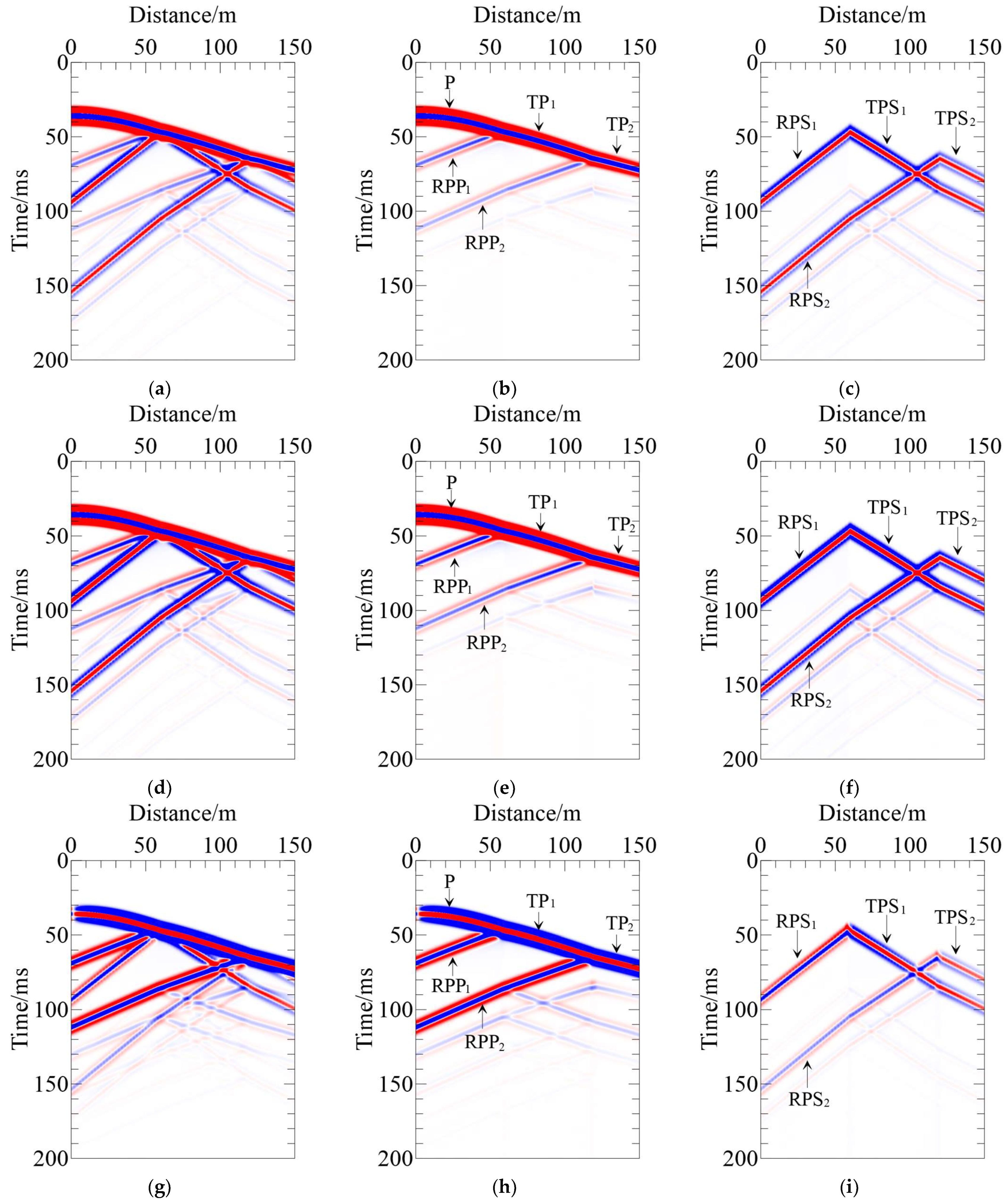
3.2. Discussion on the Imaging Results under Various Imaging Conditions

The model depicted in Figure 7 was established to analyze the validity of each imaging result. It comprises a two-layer model with a computational domain of 100.0 m × 100.0 m × 80.0 m. The physical properties of the two layers from top to bottom are P-wave velocities of 2200.0 m/s and 2600.0 m/s, S-wave velocities of 1200.0 m/s and 1450.0 m/s, densities of 1800.0 kg/m³ and 2000.0 kg/m³, respectively. The interface depth is 60.0 m. The parameters used for the forward modeling and RTM image are consistent with those described in Section 3.1.

3.2.1. Imaging Results Obtained Utilizing Vector Velocity Fields

Numerical simulation and imaging were conducted using the observational system described above, and the results obtained with the imaging strategy in Section 2.3.1 are shown in Figure 8. Due to the implementation of single-shot recordings, the completeness of the in-well 3D imaging results and the visual depiction of the structure may not be as good as conventional surface-based imaging. However, an interface can be observed at a depth of 60.0 m despite relatively low continuity. This limitation is due to the constraints imposed by the cross-well observation system. I_xx and I_yy exhibit a significant similarity, differing only by 90 degrees in orientation, which aligns with the expected theoretical results. These two components rely heavily on the v_x and v_y components, highlighting the imaging results of PS-waves. However, since the seismic source is centered at XOY plane and the receiving well is located at the outer boundary, the central region of the model lacks crucial wavefield information, making it unsuitable for imaging. As a result, imaging can only be performed in the boundary region. The imaging results for I_zz are mainly dependent on the v_z component, thus primarily representing the imaging results of PP-waves. Similarly, imaging in the central region of the model is not feasible due to the absence of wavefield information. Furthermore, high levels of noise can be observed in the imaging results. This noise originates from the direct correlation imaging of velocity components, leading to interference among different wave modes and a large number of noise artifacts. As a result, the quality of the imaging results is compromised. The lack of a clear physical interpretation of the offset imaging results, represented by the horizontal and vertical components, hinders subsequent tasks such as interpretation and inversion.

3.2.2. Imaging Results Obtained Utilizing Scalar and Vector Potentials

Figure 9 illustrates the imaging results obtained using the imaging strategy described in Section 2.3.2. It can be seen that due to the implementation of single-shot recordings and the constraints of the cross-well observation system, the 3D imaging results within the well have relatively poor interface continuity. The imaging results of the PP-waves are close to the source well area, while those of the PS-waves are close to the receiver well area, consistent with the actual situation. Due to the interferences among different mode waves, the imaging results of PS-waves exhibit significantly higher noise levels compared to those of PP-waves. In 3D space, both the imaging interfaces of PP- and PS-waves exhibit polarity reversals. This phenomenon poses challenges for the stacking of multiple shots.

3.2.3. Imaging Results Obtained Using Pure Vector P- and S-Wave

The P-wave components (I_xP, I_yP, and I_zP) were imaged in various directions and modes using the imaging strategy outlined in Section 2.3.3. The results are presented in Figure 10a–c. Additionally, the imaging results for the S-wave components (I_xS, I_yS, and I_zS) are depicted in Figure 10d–e. It can be observed that the imaging results of the six components in Figure 10 are relatively similar to those in Figure 8. The imaging results of the two horizontal components also exhibit a 90° rotation, and the central region of the model still lacks wavefield information. It can be clearly observed that employing the separated wave equations and utilizing either pure compressional or shear waves as boundary conditions results in images with significantly reduced noise levels compared to Figure 8. The separated wave equations and the input of single-mode waves effectively reduce interferences in imaging, significantly increasing the signal-to-noise ratio of the imaging results. However, different directions and modes produce more images, and the physical significance of the offset imaging results expressed by the two horizontal components and the vertical component is unclear, which is inconducive to the superimposition of the imaging results.

3.2.4. Imaging Results Obtained Using Scalarizing Vector Wavefields

In order to achieve easier stacking of multiple shots and clearer physical interpretation of the imaging results, the imaging strategy described in Section 2.3.4 was implemented. This strategy involved converting the vectorial P-waves and vectorial S-waves into scalar quantities. The scalarized imaging results for PP-waves and PS-waves are illustrated in Figure 11. It is evident from Figure 11a,b that the scalarized imaging results of PP-waves and PS-waves are relatively continuous and have no directionality. This characteristic facilitates the stacking of multiple shots after imaging. In addition, the τ_p component can be extracted from the wavefield using the auxiliary variables method, which is also applicable for imaging purposes. The imaging results obtained using this component are illustrated in Figure 11c. The imaging results for the τ_p component are similar to the imaging results of PP-waves, with an improved signal-to-noise ratio and continuity. These results can be effectively employed in subsequent applications.

According to the four different imaging results mentioned above, firstly, the imaging results by vector velocity fields exhibit significant noise, resulting in low-quality images. Furthermore, the imaging results lack clear physical meaning, which hinders subsequent interpretation and inversion tasks. Secondly, the imaging by scalar and vector potentials show relatively poor interface continuity, with polarity reversals observed on both the imaging interfaces of PP waves and PS waves. Moreover, the imaging results by pure vector P- and S-waves exhibit a high-quality representation with minimal noise interference. However, the physical significance of the imaging results is also unclear. Finally, the imaging results by scalarizing vector wavefields exhibit a high degree of continuity and lack directional bias. This characteristic makes them more suitable for superposition, enabling easier overlaying of multiple images and facilitating a clearer physical interpretation of the imaging results.

3.3. RTM Imaging Artifacts Attenuation

Figure 12 compares the pre- and post-denoised imaging profiles of single-shot PP-waves. It can be seen that without noise suppression, the imaging profiles exhibit a large amount of low-frequency noise with high energy. This noise is mainly distributed above the interfaces, significantly interfering with the imaging quality of the interfaces. By employing the Poynting vector to suppress the reflected waves and applying Laplace filtering, the low-frequency noise is effectively eliminated. Consequently, the imaging effect is improved, and the actual position and tilt angle of the interface are more accurately reflected.

4. Multiple Sensors Cross-Well 3D RTM Image Results and Analysis

In this section, we first discuss the sensor settings and design of the observation system for 3D cross-well seismic exploration. Subsequently, using the observation system, we conduct 3D imaging of layered media model and high-velocity ellipsoidal boulder models. Meanwhile, a comprehensive and detailed analysis of the imaging results is provided.

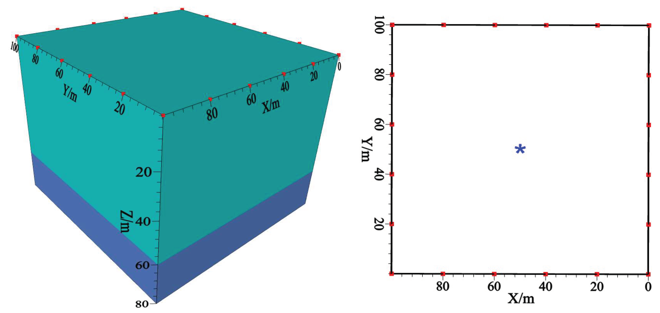
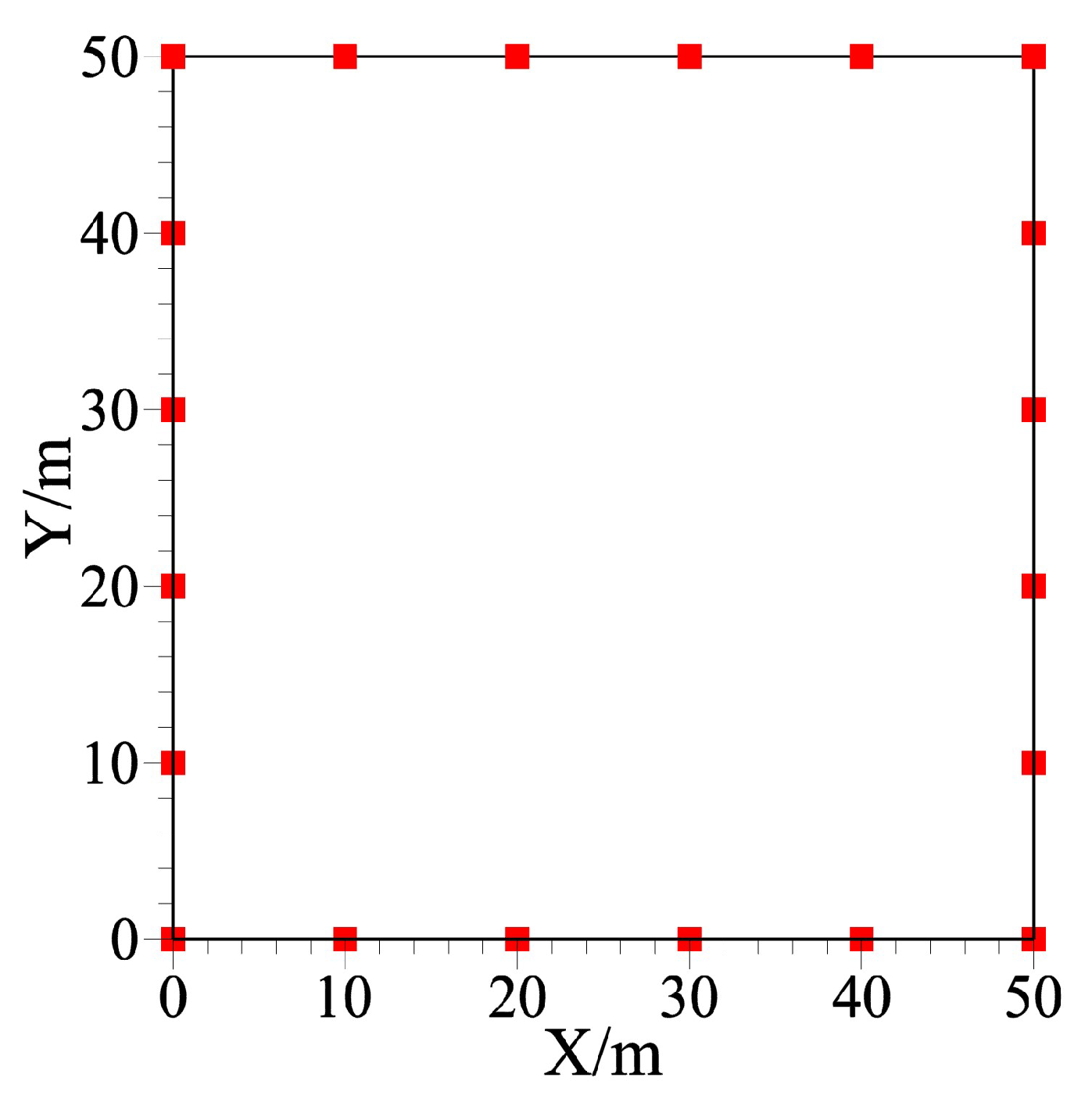
4.1. Sensor Settings and Observation System

The cross-well seismic observation system distinguishes itself from the surface-based 3D seismic methods by enabling the large-scale and high-density deployment of seismic acquisition lines. However, the cross-well seismic observation system is influenced by the actual well layout. Based on practical engineering considerations, this paper discusses the layout of the 3D multi-sensors cross-well observation system in commonly encountered square exploration areas, as depicted in Figure 13. Within a 50.0 m × 50.0 m square plane, a total of 20 well locations were arranged for the analysis. The specific coordinates of each well in the XOY plane can be found in

Table 1. The well locations within the square area in the XOY plane.

No.	Well-1	Well-2	Well-3	Well-4	Well-5	Well-6	Well-7	Well-8	Well-9	Well-10
X	0.0	10.0	20.0	30.0	40.0	50.0	0.0	10.0	20.0	30.0
Y	0.0	0.0	0.0	0.0	0.0	0.0	50.0	50.0	50.0	50.0
No.	Well-11	Well-12	Well-13	Well-14	Well-15	Well-16	Well-17	Well-18	Well-19	Well-20
X	40.0	50.0	0.0	0.0	0.0	0.0	50.0	50.0	50.0	50.0
Y	50.0	50.0	10.0	20.0	30.0	40.0	10.0	20.0	30.0	40.0

. The data acquisition was performed in the following steps: Initially, the source was subjected to an explosion in Well-1, while the other 19 were used to receive seismic signals. Then, the source was sequentially moved to the next well, and the remaining 19 wells continued to receive the seismic signals. This process lasted until Well-20 was reached.

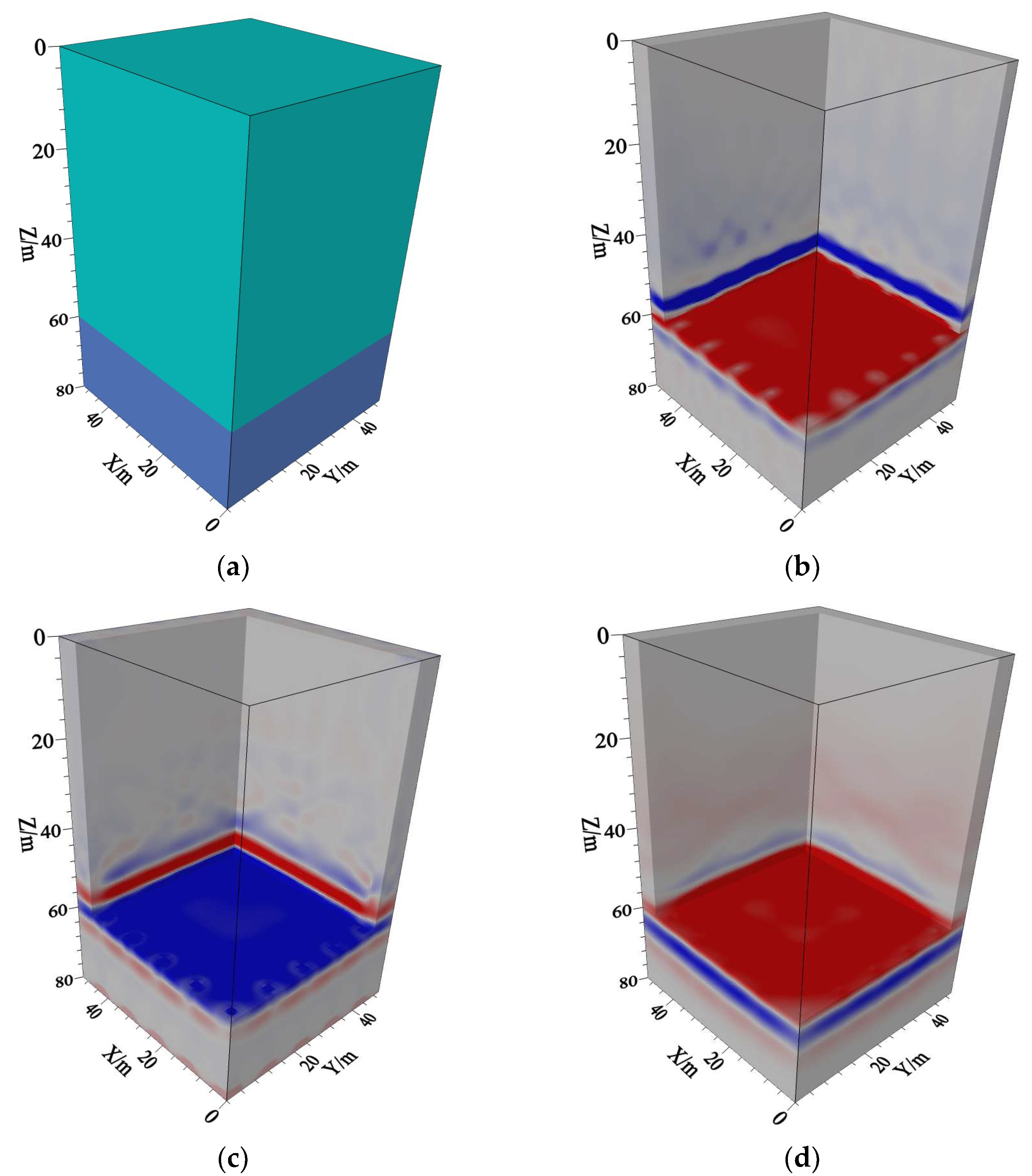
4.2. Layered Medium Model

Figure 14a illustrates a 3D layered medium model. The physical parameters of the two layers from top to bottom are as follows: P-wave velocities of 2200.0 m/s and 2600.0 m/s, S-wave velocities of 1200.0 m/s and 1450.0 m/s, densities of 1800.0 kg/m³ and 2000.0 kg/m³, and an interface depth of 60.0 m. After removing the direct waves from the recordings, the decoupled 3D elastic wave equation RTM can be used to image the layered medium in 3D across walls. The corresponding imaging results are presented in Figure 14b–d. Among them, Figure 14b depicts the imaging results for PP-waves, Figure 14c illustrates the imaging results for PS-waves, and Figure 14d shows the imaging results for τ_p. The wavefield energy is precisely concentrated at the actual interface, which is very similar to the real model. This observation result indicates that using cross-well elastic wave data and sensors can ensure accurate imaging of the 3D cross-well layered medium, encompassing both P- and S-waves. The accurate imaging results demonstrate the feasibility of the proposed method. Notably, the source locations are all positioned above the interface, and the imaging results successfully reveal the structural characteristics of the underlying interface. Compared to the traditional first-arrival travel-time imaging method, the RTM imaging method based on reflected waves has a wider exploration range. It eliminates the depth limitation of traditional observing systems for exploration.

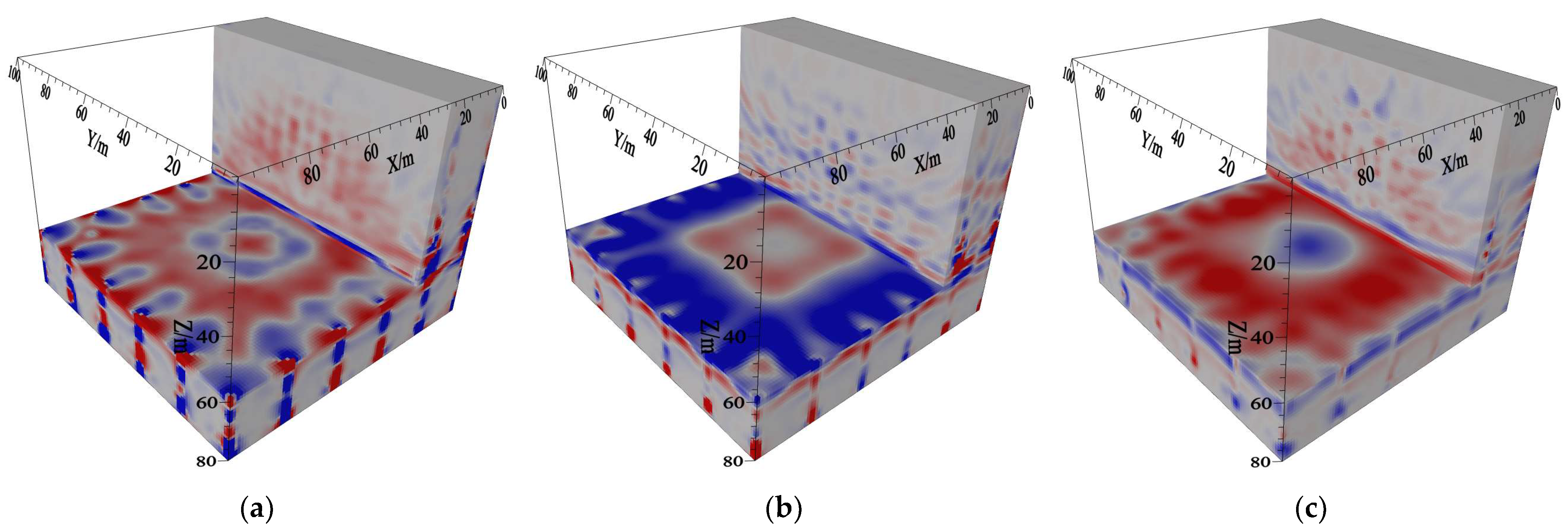
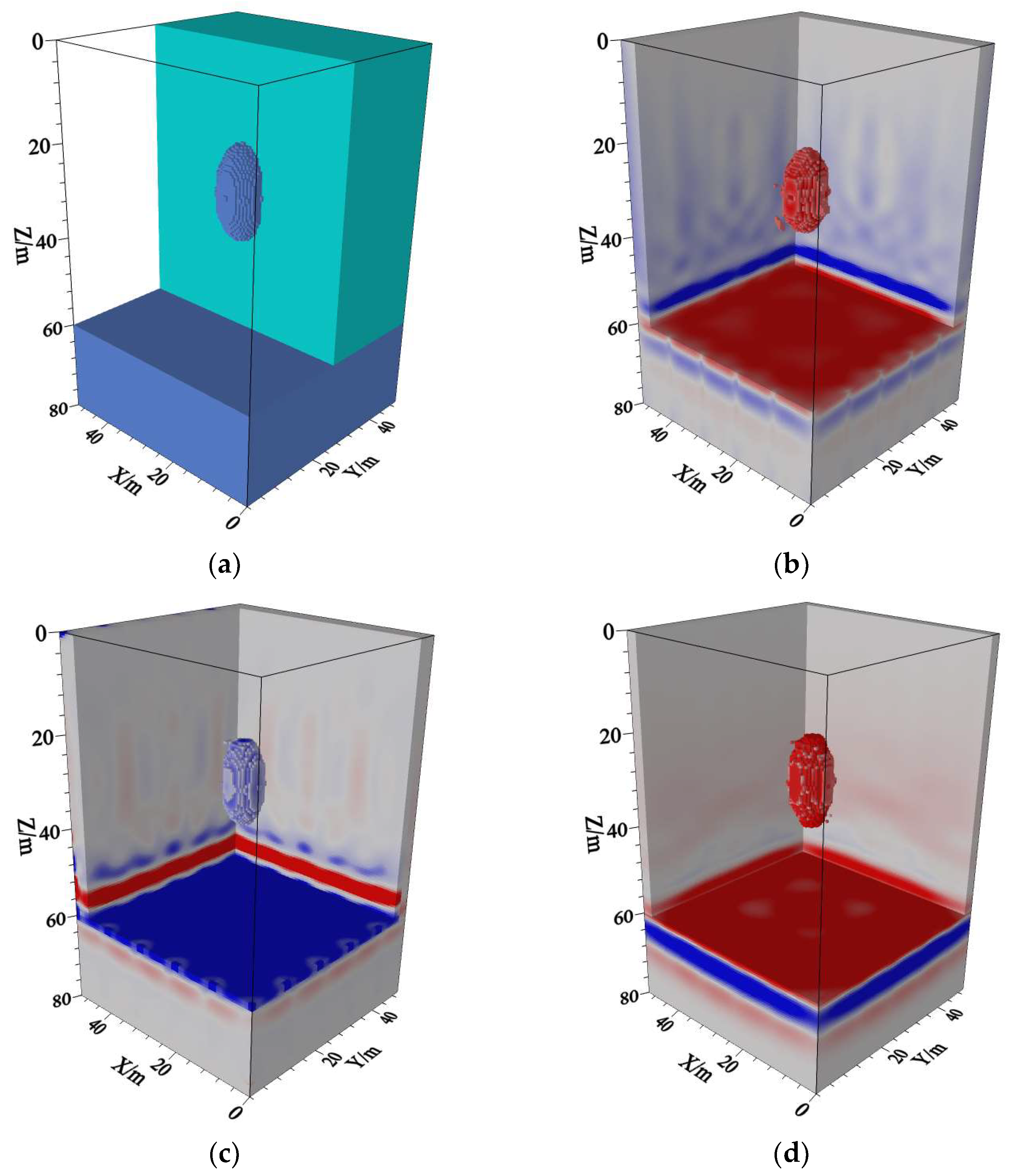
4.3. High-Velocity Ellipsoid Boulder Model

Figure 15 displays the high-velocity ellipsoid boulder model. The physical parameters of the two layers from top to bottom are as follows: P-wave velocities of 2200.0 m/s and 2600.0 m/s, S-wave velocities of 1200.0 m/s and 1450.0 m/s, densities of 1800.0 kg/m³ and 2000.0 kg/m³, and an interface depth of 60.0 m. The high-speed ellipsoidal boulder has three axis radii: a = b = 5.0 m, c = 10.0 m. The ellipsoidal body is centered at (25.0 m, 25.0 m, 30.0 m). The physical properties of the ellipsoidal body match those of the second-layer medium. After eliminating the direct waves from the recorded data, the cross-well 3D elastic wave imaging results for the high-velocity ellipsoid boulder can be obtained using the decoupled 3D elastic wave RTM equation. These results are illustrated in Figure 15b–d. Specifically, Figure 15b depicts the imaging result of the PP-wave, Figure 15c illustrates the imaging result of the PS-wave, and Figure 15d shows the imaging result of τ_p. It can be seen that the wavefield energy is concentrated at the interfaces and the position of the ellipsoid boulder in the center. The locations of the interfaces align with those of the coherent events, demonstrating a high consistency with the actual model. Based on this result, it can be concluded that the 3D cross-well elastic wave RTM imaging method with multiple wells and sensors can capture the P- and S-wave structures of localized heterogeneous bodies and perform 3D imaging. In addition to horizontal interfaces, the geological structures of lateral media are effectively revealed, and variations in lateral structures are accurately characterized. Moreover, the limitations of traditional 2D imaging methods in imaging lateral media are successfully addressed. In conclusion, the proposed method provides a fundamental basis for extracting dynamic parameters and facilitates the acquisition of comprehensive geological and geophysical information about 3D geological structures. Therefore, this method can be used as a theoretical reference and a solid foundation for detecting the geological formations of high-velocity ellipsoid boulders, especially in the field of engineering exploration.

5. Conclusions

In coastal engineering, a large amount of unsaturated loose sediments (plentiful sand) in the coastal zone leads to a strong attenuation of seismic waves. It poses significant challenges for ground seismic methods to transmit sufficient energy through the weathered zone to reach the desired depth. Compared to surface seismic reflection or refraction surveys, cross-well seismic acquisition methods emerge as an optimal choice for effectively targeting specific coastal areas. However, current studies on cross-well RTM imaging are limited to 2D space or 3D P-wave RTMs. To address the limitations of current studies, this study proposed the 3D cross-well elastic RTM imaging based on a multi-wave and multi-component technique in coastal engineering exploration. The practical benefit of this method is the utilization of the Earth’s elastic medium without increasing costs, which is used to obtain information about the distribution of subsurface rock layers, interfaces, and other structures in coastal engineering projects. Importantly, this can be achieved without resorting to extensive excavation or drilling operations.

Firstly, based on the vector decoupled elastic wave equation, this study compares and analyzes the amplitude-preserving separation algorithms for P- and S-waves implemented using the direct decomposition method and the auxiliary variable method. The wavefield decoupling algorithm achieves accurate separation of vector P- and S-waves without introducing any distortions in amplitude and phase. This feature facilitates accurate imaging of P- and S-waves in subsequent stages. Moreover, the algorithm incorporating intermediate variables integrates the P-wave pressure equation into the traditional elastic wave equations, offering significant advantages for independent imaging in the later stages. Then, this study focuses on analyzing four imaging methods under cross-correlation imaging conditions in RTM. The imaging performances of these four types of imaging strategies are compared and analyzed using experimental models. The results indicate that well-defined P- and S-wave imaging profiles can be obtained using scalarizing vector wavefield imaging conditions, and the imaging results have unique physical significance. Finally, the layer model and high-velocity ellipsoid boulder model were subjected to an RTM imaging experiment. The results indicate that the proposed 3D elastic wave imaging method can effectively generate accurate 3D cross-well profiles of P- and S-waves, thus accurately describing the geological structure. The implementation of multi-wave and multi-component RTM imaging significantly improves the utilization of wavefield information during the imaging process, thereby providing novel insights for cross-well seismic exploration. Moreover, abundant geological and geophysical information can be obtained for analyzing and interpreting 3D geological structures in coastal areas. The findings of this study have crucial theoretical significance and practical implications for exploration and development in real-world production, as well as for the investigation of geological structures in coastal engineering projects.

References

1. Esteban, M.D.; López-Gutiérrez, J.-S.; Negro, V.; Neves, M.G. Coastal Engineering: Sustainability and New Technologies. J. Mar. Sci. Eng. 2023, 11, 1562. [Google Scholar] [CrossRef]
2. Sun, Q.; Wang, Q.; Shi, F.; Alves, T.; Gao, S.; Xie, X.; Wu, S.; Li, J. Runup of landslide-generated tsunamis controlled by paleogeography and sea-level change. Commun. Earth Environ. 2022, 3, 244. [Google Scholar] [CrossRef]
3. Dong, Y. Reseeding of particles in the material point method for soil–structure interactions. Comput. Geotech. 2020, 127, 103716. [Google Scholar] [CrossRef]
4. Wang, H.; Lin, J.; Dong, X.; Lu, S.; Li, Y.; Yang, B. Seismic velocity inversion transformer. Geophysics 2023, 88, R513–R533. [Google Scholar] [CrossRef]
5. Nakata, R.; Jang, U.; Lumley, D.; Mouri, T.; Nakatsukasa, M.; Takanashi, M.; Kato, A. Seismic Time-Lapse Monitoring of Near-Surface Microbubble Water Injection by Full Waveform Inversion. Geophys. Res. Lett. 2022, 49, e2022GL098734. [Google Scholar] [CrossRef]
6. Wang, W.; Ma, J. Velocity model building in a crosswell acquisition geometry with image-trained artificial neural networks. Geophysics 2020, 85, U31–U46. [Google Scholar] [CrossRef]
7. Habib, M.A.; Zarillo, G.A. Construction of a Real-Time Forecast Model for Coastal Engineering and Processes Nested in a Basin Scale Model. J. Mar. Sci. Eng. 2023, 11, 1263. [Google Scholar] [CrossRef]
8. Liu, J.P.; Wang, Y.Y.; Liu, Z.; Pan, X.K.; Zong, Y.Q. Progress and application of near-surface reflection and refraction method. Chin. J. Geophys. 2015, 58, 3286–3305. [Google Scholar]
9. Lu, A.; Asli, B.H.S. Seismic Image Identification and Detection Based on Tchebichef Moment Invariant. Electronics 2023, 12, 3692. [Google Scholar] [CrossRef]
10. Huang, G.; Chen, X.; Luo, C.; Bai, M.; Chen, Y. Time-lapse seismic difference-and-joint prestack AVA inversion. IEEE Trans. Geosci. Remote Sens. 2020, 59, 9132–9143. [Google Scholar] [CrossRef]
11. Li, G.; Cai, H.; Li, C.F. Alternating joint inversion of controlled-source electromagnetic and seismic data using the joint total variation constraint. IEEE Trans. Geosci. Remote Sens. 2019, 57, 5914–5922. [Google Scholar] [CrossRef]
12. da Silva, J.A., Jr.; Poliannikov, O.V.; Fehler, M.; Turpening, R. Modeling scattering and intrinsic attenuation of crosswell seismic data in the Michigan Basin. Geophysics 2018, 83, WC15–WC27. [Google Scholar] [CrossRef]
13. Zhang, X.; Zheng, Z.; Wang, L.; Cui, H.; Xie, X.; Wu, H.; Liu, X.; Gao, B.; Wang, H.; Xiang, P. A Quasi-Distributed optic fiber sensing approach for interlayer performance analysis of ballastless Track-Type II plate. Opt. Laser Technol. 2024, 170, 110237. [Google Scholar] [CrossRef]
14. Angioni, T.; Rechtien, R.D.; Cardimona, S.J.; Luna, R. Crosshole seismic tomography and borehole logging for engineering site characterization in Sikeston, MO, USA. Tectonophysics 2003, 368, 119–137. [Google Scholar] [CrossRef]
15. Chen, H.; Hu, Y.; Jin, J.; Ran, Q.; Yan, L. Fine stratigraphic division of volcanic reservoir by uniting of well data and seismic data—Taking volcanic reservoir of member one of Yingcheng Formation in Xudong area of Songliao Basin for an example. J. Earth Sci. 2014, 25, 337–347. [Google Scholar] [CrossRef]
16. Sagong, M.; Park, C.S.; Lee, B.; Chun, B.-S. Cross-hole seismic technique for assessing in situ rock mass conditions around a tunnel. Int. J. Rock Mech. Min. Sci. 2012, 53, 86–93. [Google Scholar] [CrossRef]
17. Marelli, S.; Manukyan, E.; Maurer, H.; Greenhalgh, S.A.; Green, A.G. Appraisal of waveform repeatability for crosshole and hole-to-tunnel seismic monitoring of radioactive waste repositories. Geophysics 2010, 75, Q21–Q34. [Google Scholar] [CrossRef]
18. Lin, J.; Ma, R.; Sun, Z.; Tang, L. Assessing the connectivity of a regional fractured aquifer based on a hydraulic conductivity field reversed by multi-well pumping tests and numerical groundwater flow modeling. J. Earth Sci. 2023, 34, 1926–1939. [Google Scholar] [CrossRef]
19. Pongrac, B.; Gleich, D.; Malajner, M.; Sarjaš, A. Cross-Hole GPR for Soil Moisture Estimation Using Deep Learning. Remote Sens. 2023, 15, 2397. [Google Scholar] [CrossRef]
20. Binley, A.; Hubbard, S.S.; Huisman, J.A.; Revil, A.; Robinson, D.A.; Singha, K.; Slater, L.D. The emergence of hydrogeophysics for improved understanding of subsurface processes over multiple scales. Water Resour. Res. 2015, 51, 3837–3866. [Google Scholar] [CrossRef]
21. Liu, Q.; Hu, L.; Bayer, P.; Xing, Y.; Qiu, P.; Ptak, T.; Hu, R. A numerical study of slug tests in a three-dimensional heterogeneous porous aquifer considering well inertial effects. Water Resour. Res. 2020, 56, e2020WR027155. [Google Scholar] [CrossRef]
22. Zhai, J.; Wang, Q.; Xie, X.; Qin, H.; Zhu, T.; Jiang, Y.; Ding, H. A New Method for 3D Detection of Defects in Diaphragm Walls during Deep Excavations Using Cross-Hole Sonic Logging and Ground-Penetrating Radar. J. Perform. Constr. Facil. 2023, 37, 04022065. [Google Scholar] [CrossRef]
23. Luo, N.; Zhao, Z.; Illman, W.A.; Zha, Y.; Mok, C.M.W.; Yeh, T.-C.J. Three-Dimensional Steady-State Hydraulic Tomography Analysis with Integration of Cross-Hole Flowmeter Data at a Highly Heterogeneous Site. Water Resour. Res. 2023, 59, e2022WR034034. [Google Scholar] [CrossRef]
24. White, D.; Daley, T.M.; Paulsson, B.; Harbert, W. Borehole seismic methods for geologic CO2 storage monitoring. Lead. Edge 2021, 40, 434–441. [Google Scholar] [CrossRef]
25. Liu, X.; Liu, S.; Tian, S.; Zhao, Q.; Lu, Q.; Wang, K. Slowness High-resolution Tomography of Cross-hole Radar Based on Deep Learning. IEEE Geosci. Remote Sens. Lett. 2024, 21, 3000505. [Google Scholar] [CrossRef]
26. Becht, A.; Bürger, C.; Kostic, B.; Appel, E.; Dietrich, P. High-resolution aquifer characterization using seismic cross-hole tomography: An evaluation experiment in a gravel delta. J. Hydrol. 2007, 336, 171–185. [Google Scholar] [CrossRef]
27. Cheng, F.; Peng, D.; Yang, S. 3D Reverse-Time Migration Imaging for Multiple Cross-Hole Research and Multiple Sensor Settings of Cross-Hole Seismic Exploration. Sensors 2024, 24, 815. [Google Scholar] [CrossRef]
28. Cheng, F.; Liu, J.; Wang, J.; Zong, Y.; Yu, M. Multi-hole seismic modeling in 3-D space and cross-hole seismic tomography analysis for boulder detection. J. Appl. Geophys. 2016, 134, 246–252. [Google Scholar] [CrossRef]
29. Wang, H.; Lin, C.P.; Liu, H.C. Pitfalls and refinement of 2D cross-hole electrical resistivity tomography. J. Appl. Geophys. 2020, 181, 104143. [Google Scholar] [CrossRef]
30. Bae, H.S.; Kim, W.-K.; Son, S.-U.; Park, J.-S. Imaging of Artificial Bubble Distribution Using a Multi-Sonar Array System. J. Mar. Sci. Eng. 2022, 10, 1822. [Google Scholar] [CrossRef]
31. Zhong, Y.; Gu, H.; Liu, Y.; Luo, X.; Mao, Q. Elastic reverse time migration method in vertical transversely isotropic media including surface topography. Geophys. Prospect. 2022, 70, 1528–1555. [Google Scholar] [CrossRef]
32. Shin, Y.; Ji, H.-G.; Park, S.-E.; Oh, J.-W. 4D Seismic Monitoring with Diffraction-Angle-Filtering for Carbon Capture and Storage (CCS). J. Mar. Sci. Eng. 2023, 11, 57. [Google Scholar] [CrossRef]
33. Wang, Y.; Hu, X.; Harris, J.M.; Zhou, H. Crosswell seismic imaging using Q-compensated viscoelastic reverse time migration with explicit stabilization. IEEE Trans. Geosci. Remote Sens. 2022, 60, 1–11. [Google Scholar] [CrossRef]
34. Cao, L.; Li, X.; Cao, H.; Liu, L.; Wei, T.; Yang, X. 3-D Crosswell electromagnetic inversion based on IRLS norm sparse optimization algorithms. J. Appl. Geophys. 2023, 214, 105072. [Google Scholar] [CrossRef]
35. Li, X.; Lei, X.; Li, Q.; Chen, D. Influence of bedding structure on stress-induced elastic wave anisotropy in tight sandstones. J. Rock Mech. Geotech. Eng. 2021, 13, 98–113. [Google Scholar] [CrossRef]
36. Sun, R.; McMechan, G.A.; Hsiao, H.; Chow, J. Separating P- and S-waves in prestack 3D elastic seismograms using divergence and curl. Geophysics 2004, 69, 286–297. [Google Scholar] [CrossRef]
37. Sun, R.; McMechan, G.A.; Lee, C.-S.; Chow, J.; Chen, C.-H. Prestack scalar reverse-time depth migration of 3D elastic seismic data. Geophysics 2006, 71, S199–S207. [Google Scholar] [CrossRef]
38. Zong, Z.; Ji, L. Model parameterization and amplitude variation with angle and azimuthal inversion in orthotropic media. Geophysics 2021, 86, R1–R14. [Google Scholar] [CrossRef]
39. Asli, B.H.S.; Flusser, J.; Zhao, Y. 2-D Generating Function of the Zernike Polynomials and their Application for Image Classification. In Proceedings of the 2019 Ninth International Conference on Image Processing Theory, Tools and Applications (IPTA), Istanbul, Turkey, 6–9 November 2019; pp. 1–6. [Google Scholar]
40. Alterman, Z.; Karal, F.C. Propagation of elastic waves in layered media by finite difference methods. Bull. Seismol. Soc. Am. 1968, 58, 367–398. [Google Scholar]
41. Furumura, T.; Takenaka, H. A wraparound elimination technique for the pseudospectral wave synthesis using an antiperiodic extension of the wavefield. Geophysics 1995, 60, 302–307. [Google Scholar] [CrossRef]
42. Tan, C.J.; Aslian, A.; Honarvar, B.; Puborlaksono, J.; Yau, Y.H.; Chong, W.T. Estimating surface hardening profile of blank for obtaining high drawing ratio in deep drawing process using FE analysis. IOP Conf. Ser. Mater. Sci. Eng. 2015, 103, 012047. [Google Scholar] [CrossRef]
43. Seriani, G.; Priolo, E. Spectral element method for acoustic wave simulation in heterogeneous media. Finite Elem. Anal. Des. 2012, 16, 337–348. [Google Scholar] [CrossRef]
44. Bouchon, M.; Campillo, M.; Gaffet, S. A boundary integral equation-discrete wavenumber representation method to study wave propagation in multilayered media having irregular interfaces. Geophysics 1989, 54, 1134–1140. [Google Scholar] [CrossRef]
45. Pan, X.; Lu, C.; Zhang, G.; Wang, P.; Liu, J. Seismic characterization of naturally fractured reservoirs with monoclinic symmetry induced by horizontal and tilted fractures from amplitude variation with offset and azimuth. Surv. Geophys. 2022, 43, 815–851. [Google Scholar] [CrossRef]
46. Chen, J.B.; Cao, J. An average-derivative optimal scheme for modeling of the frequency-domain 3D elastic wave equation. Geophysics 2018, 83, T209–T234. [Google Scholar] [CrossRef]
47. Yang, J.; He, X.; Chen, H. Crosswell frequency-domain reverse time migration imaging with wavefield decomposition. J. Geophys. Eng. 2023, 20, 1279–1290. [Google Scholar] [CrossRef]
48. Gu, B.; Li, Z.; Ma, X.; Liang, G. Multi-component elastic reverse time migration based on the P-and S-wave separated velocity-stress equations. J. Appl. Geophys. 2015, 112, 62–78. [Google Scholar] [CrossRef]
49. Xiao, X.; Leaney, W.S. Local vertical seismic profiling (VSP) elastic reverse-time migration and migration resolution: Salt-flank imaging with transmitted P-to-S waves. Geophysics 2010, 75, S35–S49. [Google Scholar] [CrossRef]
50. Du, Q.; Guo, C.; Zhao, Q.; Gong, X.; Wang, C.; Li, X.-Y. Vector-based elastic reverse time migration based on scalar imaging condition. Geophysics 2017, 82, S111–S127. [Google Scholar] [CrossRef]
51. Wang, W.; McMechan, G.A.; Zhang, Q. Comparison of two algorithms for isotropic elastic P and S vector decomposition. Geophysics 2015, 80, T147–T160. [Google Scholar] [CrossRef]
52. Peng, D.; Cheng, F.; She, X.; Zheng, Y.; Tang, Y.; Fan, Z. Three-Dimensional Ultrasonic Reverse-Time Migration Imaging of Submarine Pipeline Nondestructive Testing in Cylindrical Coordinates. J. Mar. Sci. Eng. 2023, 11, 1459. [Google Scholar] [CrossRef]
53. Claerbout, J.F. Toward a unified theory of reflector mapping. Geophysics 1971, 36, 467–481. [Google Scholar] [CrossRef]
54. Moradpouri, F.; Moradzadeh, A.; Pestana, R.; Ghaedrahmati, R.; Monfared, M.S. An improvement in wavefield extrapolation and imaging condition to suppress reverse time migration artifacts. Geophysics 2017, 82, S403–S409. [Google Scholar] [CrossRef]
Figure 1. The flowchart illustrating the imaging process using pure vector P- and S-waves.
Jmse 12 00522 g001
Figure 2. The flowchart illustrating the imaging process using scalarizing vector wavefields.
Jmse 12 00522 g002
Figure 3. The layered model. (a) XOZ plane; (b) YOZ plane.
Jmse 12 00522 g003
Figure 4. Cross-well three-component recordings and decomposed P- and S-wave recordings. (ac) vx component; (df) vy component; (gi) vz component.
Jmse 12 00522 g004
Figure 5. The seismic trace comparison between the cross-well Vz component and the Vpz and Vsz components.
Jmse 12 00522 g005
Figure 6. (a) The single-trace comparison plot; (b) the record of the τp component within the well.
Jmse 12 00522 g006
Figure 7. Schematic representation of a layered model and an observational system. The small red rectangle represents the position of the wells. The blue asterisk represents the location of the source.
Jmse 12 00522 g007
Figure 8. Imaging results obtained using vector velocity fields for all three components. (a) Ixx component imaging results; (b) Iyy component imaging results; (c) Izz component imaging results.
Jmse 12 00522 g008
Figure 9. Imaging results obtained utilizing scalar and vector potentials. (a) PP-wave imaging results; (b) PS-wave imaging results.
Jmse 12 00522 g009
Figure 10. Imaging results obtained using pure vector P- and S-waves. (a) IxP component imaging results; (b) IyP component imaging results; (c) IzP component imaging results; (d) IxS component imaging results; (e) IyS component imaging results; (f) IzS component imaging results.
Jmse 12 00522 g010aJmse 12 00522 g010b
Figure 11. Imaging results obtained utilizing pure vector P- and S-waves. (a) PP-wave imaging results; (b) PS-wave imaging results; (c) τp component imaging results.
Jmse 12 00522 g011
Figure 12. Pre- and post-denoised imaging profiles of single-shot PP-waves: (a) image results before denoising; (b) image results after denoising.
Jmse 12 00522 g012
Figure 13. Three-dimensional multi-cross-well observation system diagram. The small red rectangle represents the position of the wells.
Jmse 12 00522 g013
Figure 14. Three-dimensional cross-well layered medium model and the elastic waves RTM imaging results. (a) Layered medium model; (b) PP-waves imaging results; (c) PS-waves imaging results; (d) τp component imaging results.
Jmse 12 00522 g014
Figure 15. Three-dimensional cross-well high-velocity ellipsoid boulder model and the elastic waves RTM imaging results. (a) High-velocity ellipsoid boulder model; (b) PP-waves imaging results; (c) PS-waves imaging results; (d) τp component imaging results.
Jmse 12 00522 g015