Short-Term Marine Wind Speed Forecasting Based on Dynamic Graph Embedding and Spatiotemporal Information

Abstract

Predicting wind speed over the ocean is difficult due to the unequal distribution of buoy stations and the occasional fluctuations in the wind field. This study proposes a dynamic graph embedding-based graph neural network—long short-term memory joint framework (DGE-GAT-LSTM) to estimate wind speed at numerous stations by considering their spatio-temporal information properties. To begin, the buoys that are pertinent to the target station are chosen based on their geographic position. Then, the local graph structures connecting the stations are represented using cosine similarity at each time interval. Subsequently, the graph neural network captures intricate spatial characteristics, while the LSTM module acquires knowledge of temporal interdependence. The graph neural network and LSTM module are sequentially interconnected to collectively capture spatio-temporal correlations. Ultimately, the multi-step prediction outcomes are produced in a sequential way, where each step relies on the previous predictions. The empirical data are derived from direct measurements made by NDBC buoys. The results indicate that the suggested method achieves a mean absolute error reduction ranging from 1% to 36% when compared to other benchmark methods. This improvement in accuracy is statistically significant. This approach effectively addresses the challenges of inadequate information integration and the complexity of modeling temporal correlations in the forecast of ocean wind speed. It offers valuable insights for optimizing the selection of offshore wind farm locations and enhancing operational and management capabilities.

1. Introduction

In recent years, as the economy and society have continued to evolve, pollution problems caused by the increased consumption of fossil fuels have grown more severe; consequently, many nations have begun to pay more attention to sustainable energy [1,2]. Regarding environmental protection, wind energy has inherent advantages over natural gas, coal, and other energy sources. To attain the objective of decarbonization by 2050, substantial expansion is anticipated in the offshore wind power sector in the coming decades [3,4]. Offshore wind possesses a greater capacity for generating wind power than terrestrial wind [5,6]. Technology for offshore wind speed forecasting that is both accurate and efficient is essential for increasing the utilization rate and economic benefits of wind energy [7,8].

The variability and stochastic nature of offshore wind speed are unavoidable consequences of numerous environmental factors. The prediction of offshore wind time series is a challenging aspect of marine forecasting and constitutes an abstract high-level regression problem [9]. The current state of wind power forecasting methods can be broadly classified into two categories: physical methods and NWP methods. Physical methods utilize NWP information to compute wind speed; however, their reliance on thermodynamics and fluid dynamics results in low efficiency and high computing expenses [10]. Physical models have a restricted capacity for short-term wind power forecasting [11] due to the high computational complexity resolved by NWP models.

Statistical and ML techniques optimize model parameters through the utilization of historical data. In addition to requiring substantial computing resources for the training procedure, forecasting models necessitate a considerable volume of sample data [12]. However, these models exhibit a rapid inference process, enabling the generation of predictions in close proximity to real time. As a result, artificial intelligence has become more significant, and neural network-based deep learning models have garnered considerable interest [13]. In the early stages of neural network research, relatively rudimentary models such as ANN [14] and BP [15] were utilized. The current domain of deep learning frequently employs more intricate deep network architectures, including CNN [16], RNN [17], and GRU [18], as a result of its development. Through the utilization of their distinctive model structures, they are capable of circumventing the gradient vanishing problem and enhancing the resistance of conventional neural networks to local optima that arise during the prediction of highly correlated wind power time series data. This renders them more appropriate for the prediction of short-term wind power output, which is distinguished by substantial data volumes and multidimensional attributes [19].

Ding et al. [20], based on the LSTM model, combined with EMD to predict the crosswind speed and downwind speed, then calculate the predicted wind direction value to achieve wind direction prediction. One month of wind monitoring data collected by the structural SHM is used to verify the effectiveness of direct prediction and indirect prediction in the prediction of wind speed and direction. Karim et al. [21] proposed a RNN prediction model combined with the dynamic adaptive Al-Biruni earth radius algorithm to predict wind power data patterns. Huang et al. [22] used an LSTM neural network to predict wind speed for each wind turbine to obtain residual values and extract time correlations of wind speed sequences. Zhu et al. [23] proposed a wind speed prediction model with spatio-temporal correlations, namely the PDCNN. This model is a unified framework that integrates CNN and MLP. Xiong et al. [24] proposed a multi-dimensional extended feature fusion model AMC-LSTM to predict wind power. The attention mechanism is used to dynamically allocate weights to physical attribute data, which effectively solves the problem that the model cannot distinguish differences in the importance of input data.

Currently, however, the majority of deep learning techniques only utilize time series data from wind sites. Nevertheless, the potential spatial dependence among wind sites must also be taken into account in practical applications [25]. As a result of their local connectivity and permutation invariance, GNNs have experienced tremendous success in modeling data relational dependencies in recent years [26].

Geng et al. [7] proposed a universal graph optimized neural network for multi-node offshore wind speed prediction—the spatio-temporal correlated graph neural network. Khodayar et al. [27] proposed a scalable graph convolutional deep learning architecture (GCDLA). This model introduces a rough set theory by approximating upper and lower bound parameters in the model. Yu et al. [28] proposed an SGNN (superposition graph neural network) for feature extraction, which can maximize the utilization of spatial and temporal features for prediction. In the four offshore wind farms used in the experiments, the mean square error of this method is reduced by 9.80% to 22.53%. Xu et al. [29] proposed a new spatio-temporal prediction model based on optimal weighted GCN and GRU, using DTW distance for constructing optimal weighted graphs between different wind power plant sites. The graph neural network in the above method effectively aggregates the spatio-temporal information, but only considers the overall correlation of the sequence when constructing the adjacency matrix and does not consider that the correlation may be different in local time.

To address the aforementioned obstacles and optimize the utilization of spatio-temporal data, this article centers on the implementation of spatio-temporal data within a graph neural network-based multi-step wind forecasting method. In order to address the issue of inadequate local information capture, this study introduced a dynamic graph-embedding technology and developed a GAT-LSTM network structure to capture spatio-temporal information on wind speed from multiple stations. This research endeavors to produce wind speed forecasts with a greater degree of precision by generating information-enriched time series via multi-step forecasting. The overarching objective is to enable more accurate decision-making within a designated time frame. Within this framework, the objective of this research is to examine multi-step prediction. Each step will have a duration of 10 min, 1 h, and 4 h, and the pre-prediction time resolution will be 10 min.

The contributions of this paper can be summarized as:

• To address the insufficient capability in modeling complex spatio-temporal features in existing offshore wind speed prediction research, this study proposes a DGE technique. By constructing subgraphs at each time step, the model’s ability to capture local feature dependencies is effectively enhanced, achieving dynamic modeling of offshore wind fields.
• The effective integration of GAT and LSTM networks enables the model to have both the advantages of mining complex nonlinear spatial dependencies and temporal dynamic evolutions. By fully incorporating nodal modal features and topological structures, the capability of modeling temporal correlations of offshore wind fields is significantly improved, achieving accurate multi-step wind speed prediction.
• Experimental results show that on the public offshore wind speed dataset from the NDBC (National Data Buoy Center), the proposed model achieves effective multi-step wind speed prediction, verifying the applicability of the method.

2. Materials and Methods

2.1. Materials

The actual data set utilized in this article is the NDBC (https://www.ndbc.noaa.gov/historical_data.shtml (accessed on 23 December 2023)) [30] buoy data set, which comprises observations from nearly 100 moored buoys monitored by the NDBC, including 55 tropical atmosphere ocean buoys operated and maintained in the equatorial Pacific. The geographical coordinates of the beacons span from 9° N to 8° S north latitude and 95° W to 165° E longitude [31].

Wind speed data collected by buoys were used. To ensure the experiment proceeds without hiccups, this paper selects 12 buoys, including the predicted buoy No. 46042, They are distributed along the Pacific coast of North America, as shown in Figure 1. The starting time is from 1 January 2022 00:00:00 to 31 October 2022 23:50:00 every 10 min, and other basic information is shown in

Table 1. Table of basic information for each buoy.

Number of Buoy	Size	Max (m/s)	Min (m/s)	Mean (m/s)	Std (m/s)	Skewness	Kurtosis
46002	43,751	16.7	0.0	6.38	2.87	0.31	−0.13
46011	43,751	16.3	0.0	6.22	3.07	0.11	−0.84
46014	43,751	17.8	0.0	5.88	3.56	0.53	−0.52
46025	43,751	16.2	0.0	3.44	2.15	1.39	3.03
46028	43,751	17.6	0.0	7.18	3.86	0.03	−1.11
46042	43,751	15.7	0.0	6.19	3.16	0.16	−0.8
46059	43,751	14.2	0.0	6.09	2.58	0.19	−0.53
46072	43,751	20.9	0.0	5.92	3.66	0.41	−0.62
46084	43,751	21.0	0.0	6.68	3.66	0.58	−0.19
46089	43,751	19.6	0.0	6.05	2.94	0.3	−0.25
51000	43,751	12.6	0.0	6.13	2.10	−0.31	−0.44
51004	43,751	15.7	0.0	7.23	1.80	−0.41	0.79

. Although the original data contains some missing values, their number is minimal. To mitigate the risk of human error and preserve the distribution of the data, we employ the mean of the entire set of data for filling purposes, subsequent to removing any anomalies.

Based on the data presented in Table 1, it is evident that the distribution of wind speed data obtained from buoys is predominantly positively biased. This indicates that instances of high wind speed are infrequent. Simultaneously, the data exhibit a kurtosis that is comparatively small, suggesting that the wind speed value predominantly mirrors the mean value and that instances of extreme wind speed are infrequent.

Due to the fact that the majority of wind power projects are situated offshore, it is critical to choose buoys that capture weather and ocean conditions in these regions. Implementing this approach is critical for ensuring the viability and effectiveness of offshore wind energy initiatives. Through the careful selection of these offshore locations, we are capable of furnishing up-to-the-minute meteorological and oceanic data that are highly pertinent to offshore wind power endeavors. As a result, we are able to assist in the efficient organization, functioning, and upkeep of wind farms.

2.2. Methods

2.2.1. Overview

This scholarly article introduces a novel DGE-GAT-LSTM methodology for wind speed forecasting, which is founded on dynamic graph embedding. By constructing a subgraph for each time step, the method enables the model to dynamically comprehend and process the spatiotemporal properties of wind speed data. The study employs cosine similarity technology to ascertain the connection relationship among buoy points. This method aids in the precise identification and description of the dynamic relationship among various buoy points. Special emphasis is placed on the ability to handle multi-step predictions. Multi-step prediction is used to predict the wind speed at multiple time points in the future, which has important practical application value in the fields of meteorological prediction and wind energy utilization.

To enhance the efficiency of capturing and processing temporal and spatial information present in wind speed data, a string deep learning model was developed by combining a graph neural network and a long short-term memory network. By extracting both spatial and temporal features from the data, the structure of this model enhances the precision and effectiveness of wind speed forecasting.

The model entails a graph neural network component that processes and interprets the spatial information contained within the wind speed data. Meanwhile, the LSTM network is tasked with capturing the temporal dependencies and dynamic alterations present in the time series data. By utilizing this dual mechanism, the model attains a more comprehensive comprehension of the intricate patterns present in the wind speed data, thereby enabling it to generate predictions that are more precise in nature. The overall flowchart is shown in Figure 2.

The proposed DGE-GAT-LSTM model consists of two GAT network layers. The normalized data and adjacency matrix information are passed into the model, and the original dimension is changed to 64 and then 128 through the double-layer GAT network. Then, a residual connection is established to fuse the normalized result with the GAT network structure, which keeps the dimension unchanged and realizes the operation of average sum. This goal is achieved by augmenting the information into finer-grained results. To ensure the LSTM input format, the dimensions need to be grouped and split into corresponding inputs. They are then fed to the LSTM network for prediction. Then, the last time step is used as the input of the linear layer to obtain the final prediction result.

DGE technology is utilized to acquire the adjacency graph information during this procedure. To improve the model’s ability to predict local information, the side information is not set for the entire time series in this paper, but rather at each time step. In order for the model to gain a more comprehensive understanding of the properties of the local sequence, the cosine similarity is employed to ascertain the connectivity relationship among the edges in the local subsequences of the window size. The relevant calculation results are given in Algorithms 1 and 2.

Algorithm 1 Graph Data Processing
Input: $num\_nodes$$: \mathrm{Number} \mathrm{of} \mathrm{nodes}, data$$: \mathrm{Data}, columns$: Column names
Output: Graph model
1:	function$\mathrm{GraphDataProcessing}(num\_nodes, data, columns$)
2:	Initialize edge index to [[ ],[ ]]
3:	for $i$$\mathbf{from} 0 \mathbf{to} num\_nodes$ do
4:	for $j$$\mathbf{from} i+1$$\mathbf{to} num\_nodes$ do
5:	Compute correlation between data in column $i$ and column $j$
6:	Calculate correlation
7:	if Correlation $\ge$ threshold then
8:	$\hspace{1em}\hspace{1em}\hspace{1em}\mathbf{Add} \mathbf{edge} \left(i, j\right)$ to edge index
9:	end if
10:	end for
11:	end for
12:	Convert edge index to LongTensor
13:	Create graph model
14:	Ensure bidirectional relationships in the graph model
15:	return Graph model
16:	end function

Algorithm 2 Network Model Algorithm
Input: $data,num\_nodes, seq\_len, B,pred\_step\_size,columns: Data and parameters$
Output: Prediction results and ground truth
1:	function NetworkModel($data,num\_nodes, seq\_len, B, pred\_step\_size, columns$)
2:	Define GAT model and parameters: $in\_feats, h\_feats, out\_feats$
3:	Define LSTM model parameters: $args$
4:	Create GAT-LSTM model: $model$
5:	function FORWARD(data)
6:	Extract $x$,$edge\_index$, $batch$ from $item$
7:	Pass $x$,$edge\_index$ to GAT model: $x\_gat$
8:	Add $x\_gat$ to $x: x \_sum$
9:	Pass $x \_sum$ to LSTM model: $x\_lstm$
10:	Pass $x \_lstm$ to fully connected layer: $y\_pred$
11:	end function
12:	return $y\_pred$
13:	end function

2.2.2. Cosine Similarity Creates Adjacency Matrix

Cosine similarity is a frequently employed technique in data comparison, particularly when examining text and time series, for determining the degree of similarity between two vectors. The similarity between two vectors is quantified through the calculation of their angle of separation; a lesser angle signifies a greater degree of similarity.

Suppose we have two time series: $A$ and $B$, which are represented as vectors $A=\left\{A_1, A_2, A_3\dots A_n\right\}$ and $B=\left\{B_1, B_2, B_3\dots B_n\right\}$, respectively. These vectors can be represented as arrays containing data points.

• Calculate the length ||A|| of the vector A and the length ||B|| of the vector B This can be calculated using the following formula:

  $$\parallel A\parallel =\sqrt{\sum _{i=1}^n{A}_i^2}$$

  (1)

  $$\parallel B\parallel =\sqrt{\sum _{i=1}^n{B}_i^2}$$

  (2)

  where n is the number of data points in the time series, A_i and B_i are the ith data point in series A and B, respectively.

2.

Compute the inner product of vectors A and B.

$$A\cdot B=\sum _{i=1}^n{A}_i\cdot B_i$$

(3)

3.

Calculate the cosine similarity (cos_sim) using the following formula:

$$\cos \_\mathrm{sim} =\frac{A\cdot B}{\parallel A\parallel \cdot \parallel B\parallel }$$

(4)

Therefore, for nodes $i$ and $j$, their wind speed sequence in the time window is represented by $A$ and $B$. At this time, a threshold is set according to the value of cosine similarity, and the formula is as follows:

$$\mathrm{If} \cos \_\mathrm{sim} \left(i,j\right)>threshold, \mathrm{then} \left\{\begin{array}{l}1,\left|\right|\left|\right| \mathrm{Node} i \mathrm{and} \mathrm{Node} j \mathrm{are} \mathrm{adjacent} \\ 0,\left|\right|\left|\right| \mathrm{Node} i \mathrm{and} \mathrm{Node} j \mathrm{are} \mathrm{not} \mathrm{adjacent} \end{array}\right.$$

(5)

2.2.3. Graph Attention Network

GAT adopts an attention mechanism, which can assign different weights to different nodes, and relies on pairs of neighboring nodes when training without depending on the specific network structure, which can be used for inductive tasks [32]. The multi-head attention mechanism it adopts is shown in Figure 3.

Calculate attention scores for each node $i$ with respect to its neighbors $j$:

$$e_{ij}^{\left(l\right)}=\mathrm{LeakyReLU}\left({\overrightarrow{a^{\left(l\right)}}}^T\left[W^{\left(l\right)}{h}_i\parallel W^{\left(l\right)}{h}_j\right]\right)$$

(6)

Here, $h_i$ and $h_j$ are the representations of nodes $i$ and $j$ after applying the weight matrix $W^{\left(l\right)}$. $a^{\left(l\right)}$ is the learnable parameter vector used to compute attention. Nonlinearity is introduced using the LeakyReLU activation function. Softmax is used to calculate the normalized value of the attention coefficient of each node $i$ to its neighbor $j$:

$${\alpha }_{ij}^{(l)}=\frac{\exp \left(e_{ij}^{(l)}\right)}{\sum _{k\in {\mathcal{N}}_i}\exp \left(e_{ik}^{(l)}\right)}$$

(7)

Here, ${\mathcal{N}}_i$ denotes the set of neighbors of node $i$. These coefficients indicate the importance of node $i$ to its neighbors.

Aggregate the neighbors using the attention coefficient:

$$h_i^{(l+1)}=\sigma \left(\sum _{j\in {\mathcal{N}}_i}{\alpha }_{ij}^{(l)}{W}^{(l)}{h}_j\right)$$

(8)

Here, $\sigma$ is the activation function.

2.2.4. Long Short-Term Memory Network

LSTM networks are a subtype of deep learning neural networks that are particularly advantageous in time series analysis and natural language processing due to their ability to process sequential data. LSTM networks are a subtype of RNN specifically engineered to tackle the issue of long-term dependency that plagues RNN. The structure is shown in Figure 4.

The main features of LSTM networks include:

Forget gate: The LSTM determines whether or not to retain previously remembered information using the forget gate. This gate determines which data should be retained and which should be discarded from the previous memory state.

Input gate: From the current input, the input gate determines which information is to be remembered. It updates the new memory using the current input and the previous memory state.

The output gate generates the network’s output in accordance with the current input and the updated memory state. This output may be utilized as input for subsequent time steps or for additional purposes.

Cell memory: A solitary memory cell is incorporated into LSTM networks to store and transmit data. In conjunction, the forget, input, and output gates regulate the data stored in the memory cells.

Each gate’s computation is performed as follows:

$$f_i=\sigma \left(\sum W_{xf}{x}_i+\sum W_{hf}{x}_{t-1}+\sum W_{cf}{x}_{t-1}+b_f\right)f_t$$

(9)

$$i_t=\sigma \left(\sum W_{xi}{x}_t+\sum W_{hi}{x}_{t-1}+\sum W_{ci}{x}_{t-1}+b_i\right)$$

(10)

$$o_t=\sigma \left(\sum W_{xo}{x}_t+\sum W_{ho}{x}_{t-1}+\sum W_{co}{x}_{t-1}+c_0\right)$$

(11)

$$c_t=f_t{c}_{t-1}+i_t\tanh \left(\sum W_{xc}{x}_t+\sum W_{hc}{x}_{t-1}+b_c\right)$$

(12)

$$h_t=o_t\tanh \left(c_t\right)$$

(13)

In (9)–(13), $W$ represents the weight value of each layer of the neural network, and $b$ represents the bias term. $i_t$ is the forget gate, $f_t$ is the input gate, $o_t$ is the output gate, $c_t$ is the vector value of the memory cell, $tanh$ refers to the hyperbolic tangent function, and $\sigma$ is the $sigmoid$ function.

2.2.5. Direct Multi-Output Strategy

This research employed the direct method. This entailed prediction of multi-step forward data, with the preceding time step serving as the input variables and the subsequent time step being assumed to contain the target variables. For example, when making one-step predictions, the input variable $X=\left\{x_2,x_3,x_4,\dots ,x_{t-1}\right\}$ is a sequence of a size one sliding window. The $Y=\left\{y_t\right\}$ sequence for the predicted target contains only one target value. When making multi-step predictions, the sequence length of $Y$ is increased, and $Y=\left\{y_t,y_{t+1},\dots ,y_{t+5}\right\}$ and $Y=\left\{y_t,y_{t+1},\dots ,y_{t+23}\right\}$ for $t+5$ and $t+23$ step predictions as shown in the figure. As illustrated in Figure 5, the forecast data may consist of one to multiple predictions.

3. Experimental Results and Analysis

3.1. Experiment Design

All the experiments in this paper were conducted on a personal computer running on a Windows 11 operating system. The computer is equipped with a 12th Gen Intel(R) Core(TM) i7-12700 processor (Manufacturer: Intel, Santa Clara, CA, USA) and 1660 Supergraphics card (Manufacturer: Nvidia, Santa Clara, CA, USA), and uses a 256 GB SN740 NVMe WD solid state drive for storage (Manufacturer: Western Digital, San Jose, CA, USA). In addition, the PyTorch version used in this paper is 2.1, and the CUDA version is 12.1. numpy is version 1.24.4, pandas is version 2.1.4, and matplotlib is version 3.5.1.

The following experimental results are the average values obtained by repeating experiments 10 times.

3.2. Evaluation Metrics

For the purpose of assessing the performance of the model, this paper employs two evaluation indicators: MAE and RMSE. MAE exhibits enhanced robustness towards outliers or anomalies due to its construction as the mean of absolute errors, rendering it relatively unaffected by substantial error magnitudes. Since RMSE is calculated as the square root of the mean of the squared errors, it becomes more susceptible to large error values. This increases the likelihood that it will penalize significant errors, so it may more accurately reflect the model’s sensitivity to such errors in certain circumstances.

$$\mathrm{M}\mathrm{A}\mathrm{E}=\frac{1}{n}\sum _{i=1}^n|Y_i-{\hat{Y}}_i|$$

(14)

$$\mathrm{R}\mathrm{M}\mathrm{S}\mathrm{E}=\sqrt{\frac{1}{n}\sum _{i=1}^n{(Y_i-{\hat{Y}}_i)}^2}$$

(15)

where $n$ is the number of data points,$Y_{i }$ is the actual value, and ${\widehat{Y}}_i$ is the predicted value.

3.3. Experimental Results

This section will encompass the execution of the model’s experiments. To evaluate the model’s performance as advertised, two distinct groups of experiments were devised. The initial experiment is the benchmark model experiment, in which the predictive ability of the model is evaluated by comparing it to several benchmark models. Experiment 2 is the ablation experiment, in which each component of the model is progressively substituted in order to determine the effect of each component on performance.

The data used in this study span the time period from 00:00:00 1 January 2022 to 23:50:00 31 October 2022. In order to verify the generalization and robustness of the model, 2-test set cross-validation is used. This strategy can make full use of all the data, and all the data including the test set are involved in the training and evaluation process of the model. Compared with the standard time series cross-validation, the computational overhead is relatively small. Therefore, the initial 60% is designated as the training set, followed by the final 20% as the validation set, and the final 20% is divided equally into a K1-test set and a K2-test set in chronological order. The training set is used to train the model, while the validation set is used to validate the model hyperparameters to prevent overfitting and underfitting, and the test set is used to evaluate the performance of the model.

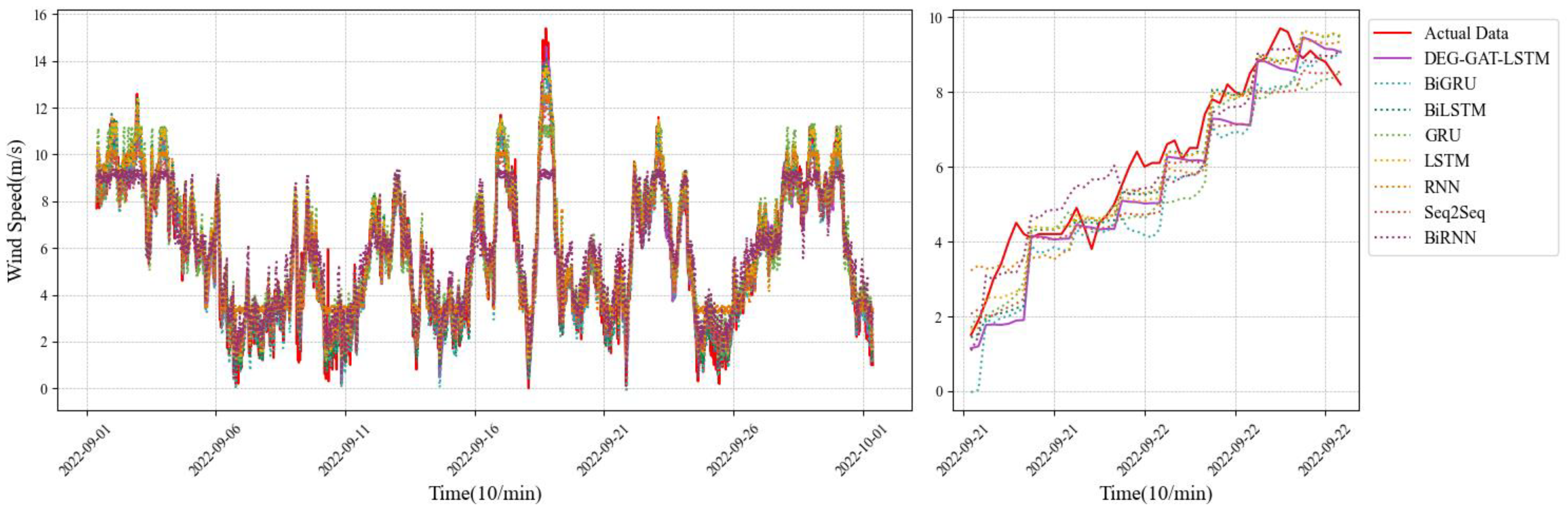
3.3.1. Experiment I

In Experiment I, the DGE-GAT-LSTM proposed in this paper will be compared with LSTM, BILSTM, GRU, RNN, BIRNN, Seq2Seq and other models, The relevant introduction of each model is as follows:

• LSTM is a recurrent neural network designed to process sequential data and capture long-term dependencies through gating units.
• BILSTM considers context information simultaneously through forward and backward LSTM layers and is suitable for a variety of sequence tasks.
• GRU is a recurrent neural network similar to LSTM with fewer parameters and a lower computational cost.
• RNN is one of the earliest sequence models, but it faces the vanishing gradient problem and is not suitable for long-term dependence tasks.
• BIRNN combines a forward and backward RNN or LSTM layers to fully understand sequence data and is suitable for a variety of tasks.
• Seq2Seq models are used for sequence-to-sequence tasks, including machine translation and speech recognition, and consist of an encoder and a decoder.

In order to achieve more convincing results in the benchmark experiment, this paper uses a grid search to search the hyperparameters of the benchmark model, aiming to find the optimal parameters to compare with the proposed model. The goal of a grid search is the number of hidden layers and the number of network layers. The search ranges are [32, 64, 128] and [1, 2, 3]. The determined optimal parameters of each benchmark model are shown in

Table 2. Detailed description of all models in Experiment I.

Model	Specific Description
LSTM	The internal parameters were randomized, 1 LSTM layer, 128 hidden dimensions, and a linear layer.
BILSTM	The internal parameters were randomized, 1 bidirectional LSTM layer, 128 hidden dimensions, and a linear layer.
GRU	The internal parameters were randomized, 3 GRU layers, 128 hidden dimensions, and one linear layer.
BIGRU	The internal parameters were randomized, 3 bidirectional GRU layers, 128 hidden dimensions, and one linear layer.
RNN	The internal parameters were randomized, 1 RNN layer, 128 hidden dimensions, and a linear layer.
BIRNN	The internal parameters were randomized, 1 bidirectional RNN layer, 128 hidden dimensions, and a linear layer.
Seq2Seq	The internal parameters were randomized, LSTM is used as encoder, 2 LSTM layers with 64 hidden dimensions and MLP is used as decoder.
DGE-GAT-LSTM	2 layers of GAT network with 4 attention heads, one layer of LSTM, GAT network and LSTM are serially connected. 2 linear layers with nonlinear activation.

.

To ensure the fairness of the experiment, the remaining hyperparameters are consistent: the epoch is 30, the sliding window size is 24, and the batch size is 24. In order to avoid over-connection, dense edges are also ensured for the subsequent extraction of spatial features. The cosine similarity threshold is 0.4. This means that there are more than 0.4 connections between nodes. This means that there is a connection between nodes greater than 0.4. The SGD optimizer was used with a learning rate of 0.005, momentum = 0.9, and weight_decay = 1 × 10⁻⁶. The prediction results are shown in

Table 3. Table of error of prediction results in Experiment I.

Model	MAE (m/s)			RMSE (m/s)
	1-Step (10 min)	6-Step (1 h)	24-Step (4 h)	1-Step (10 min)	6-Step(1 h)	24-Step (4 h)
LSTM	0.3425	0.5946	0.9801	0.4620	0.7750	1.2968
BILSTM	0.3447	0.5903	0.9493	0.4648	0.7740	1.2651
GRU	0.3561	0.7306	0.9448	0.4734	0.9412	1.2694
BIGRU	0.3570	0.5780	0.9602	0.4769	0.7633	1.2916
RNN	0.3604	0.7635	0.9789	0.4903	1.0036	1.3009
BIRNN	0.3650	0.7304	0.9527	0.4967	0.9598	1.2851
Seq2Seq	0.3450	0.5995	1.0059	0.4623	0.7837	1.3250
DGE-GAT-LSTM	0.3396	0.5571	0.9333	0.4546	0.7363	1.2501

.

The single-step prediction results are shown in Figure 6 and Figure 7, the 6-step prediction results are shown in Figure 8 and Figure 9, and the 24-step prediction results are shown in Figure 10 and Figure 11.

By examining Figure 6, Figure 7, Figure 8, Figure 9 and Figure 10 and Table 3, it is evident that the DGE-GAT-LSTM model, which was proposed, obtained the smallest MAE and RMSE values for single-step, 6-step, and 24-step predictions, respectively. This finding underscores the model’s superior performance in terms of predictions.

For a 1-step (10 min) prediction, the MAE index of DGE-GAT-LSTM model decreases by 1–7%, and the RMSE index decreases by 2–9%, respectively. For a 6-step (10 min) prediction, the MAE index of the DGE-GAT-LSTM model decreases by 6–37%, and the RMSE index decreases by 4–36%, respectively. For a 24-step (10 min) prediction, the MAE index of DGE-GAT-LSTM model decreases by 1–8%, and the RMSE index decreases by 1–6%, respectively.

Experimental results show that compared with traditional sequence prediction models (such as LSTM, BILSTM, GRU, BIGRU, etc.), the DGE-GAT-LSTM model shows superior accuracy and efficiency in each time increment in the prediction task. The results prove that the DGE-GAT-LSTM model can effectively capture the dynamic characteristics and complex dependencies in time series data through its combination of a dynamic graph embedding strategy and a graph attention network, as well as the application of a long short-term memory network when dealing with time series prediction problems, thus providing a more accurate prediction.

3.3.2. Experiment II

Principally, a comparison of ablation experiments is conducted in this experiment. To ascertain the extent to which each model component can influence the overall model, the following five model groups are established:

• Model1 purpose: The original model serves as a baseline for comparison
• Model without residuals: model2 Objective: To analyze the effect of the residual structure
• Model without graph attention: model3 Objective: To verify the effectiveness of the graph attention mechanism
• Model without LSTM: model4 Objective: To test the effect of LSTM on the model performance
• Model5 without DGE objective: To test the performance of dynamic graph embedding

Epochs are all 30, the batch size is 24, the sliding window size is 24, an Adam optimizer is used, and the learning rate is 0.001. The experimental results are shown in Figure 12 and Figure 13 and

Table 4. Table of error of prediction results in Experiment II.

Model	MAE (m/s)	Percentage	RMSE (m/s)	Percentage
	1-Step (10 min)		1-Step (10 min)
Model1	0.3419	0%	0.4549	0%
Model2	0.4298	+25.69%	0.5548	+21.96%
Model3	0.3729	+9.06%	0.5027	+10.50%
Model4	1.9339	+465.57%	2.3262	+411.37%
Model5	0.4112	+20.26%	0.5361	+17.84%

.

The MAE of Model2 is 0.4298, which is 25.69% higher than the baseline model, and the RMSE is 0.5548, which is 21.96% higher than the baseline model. This indicates that the residual structure has a positive impact on the model performance, and its absence leads to an increase in error. The MAE of Model3 is 0.3729, 9.06% higher than that of the baseline model, and RMSE is 0.5027, 10.50% higher than that of the baseline model. This shows that the graph attention mechanism plays an important role in improving the accuracy of the model. The MAE of Model4 is 1.9339, which is 465.57% higher than the baseline model, and the RMSE is 2.3262, which is 411.37% higher than the baseline model. This significant performance degradation strongly indicates that LSTM is critical to the performance of the model, which can significantly improve the accuracy and stability of prediction. The MAE and RMSE of Model5 are 0.4112, 20.26% higher than the baseline model, and 0.5361, 17.84% higher than the baseline model. This indicates that DGE also contributes positively to the model, and missing it leads to performance degradation. Therefore, residual structure, graph attention mechanism, LSTM and dynamic graph embedding are crucial for improving the prediction accuracy of the model.

4. Conclusions and Future Work

In this paper, the proposed model DGE-GAT-LSTM is evaluated through the above experiments to predict the multi-step forward wind speed at a given location of NDBC buoys through experimental simulations using real wind speed data. The direct method does not suffer from error propagation like the recursive method, so it can be used for multi-step ahead prediction. Three different long-term time horizons (1-step, 6-step, 24-step) are considered to compare the ability of the algorithm to predict wind speed. The experimental results show the superiority of the proposed model, which is better than the baseline model in most time step predictions. The effect of each component on the model can be seen through the ablation experiment of Experiment 2. Among them, the extraction of spatial information and temporal information is particularly important and the proposed dynamic graph embedding technique also improves the accuracy of the wind speed prediction.

In future work, the influence of different temporal similarities on the model performance will be considered, and some more complex parallel computing structures will be used to reduce the model computing time. A more complex and interpretable cross-validation will be used to split the dataset to ensure that the model’s ability to predict future points is fully evaluated, which better reflects the generalization ability of the model. The optimal parameter configuration for each model in future work will be investigated and the applicability in different datasets or application scenarios will be explored. The study of the model’s generalization to different seasons will be considered.

References

1. Suo, L.; Peng, T.; Song, S.; Zhang, C.; Wang, Y.; Fu, Y.; Nazir, M.S. Wind speed prediction by a swarm intelligence based deep learning model via signal decomposition and parameter optimization using improved chimp optimization algorithm. Energy 2023, 276, 127526. [Google Scholar] [CrossRef]
2. Khosravi, A.; Machado, L.; Nunes, R.O. Time-series prediction of wind speed using machine learning algorithms: A case study Osorio wind farm, Brazil. Appl. Energy 2018, 224, 550–566. [Google Scholar] [CrossRef]
3. Liu, X.; Lin, Z.; Feng, Z. Short-term offshore wind speed forecast by seasonal ARIMA—A comparison against GRU and LSTM. Energy 2021, 227, 120492. [Google Scholar] [CrossRef]
4. Peng, X.; Wang, H.; Lang, J.; Li, W.; Xu, Q.; Zhang, Z.; Cai, T.; Duan, S.; Liu, F.; Li, C. EALSTM-QR: Interval wind-power prediction model based on numerical weather prediction and deep learning. Energy 2021, 220, 119692. [Google Scholar] [CrossRef]
5. Rodrigues, S.; Restrepo, C.; Kontos, E.; Pinto, R.T.; Bauer, P. Trends of offshore wind projects. Renew. Sustain. Energy Rev. 2015, 49, 1114–1135. [Google Scholar] [CrossRef]
6. Gao, Z.; Li, Z.; Xu, L.; Yu, J. Dynamic adaptive spatio-temporal graph neural network for multi-node offshore wind speed forecasting. Appl. Soft Comput. 2023, 141, 110294. [Google Scholar] [CrossRef]
7. Geng, X.; Xu, L.; He, X.; Yu, J. Graph optimization neural network with spatio-temporal correlation learning for multi-node offshore wind speed forecasting. Renew. Energy 2021, 180, 1014–1025. [Google Scholar] [CrossRef]
8. Ren, Y.; Li, Z.; Xu, L.; Yu, J. The data-based adaptive graph learning network for analysis and prediction of offshore wind speed. Energy 2023, 267, 126590. [Google Scholar] [CrossRef]
9. Xu, L.; Ou, Y.; Cai, J.; Wang, J.; Fu, Y.; Bian, X. Offshore wind speed assessment with statistical and attention-based neural network methods based on STL decomposition. Renew. Energy 2023, 216, 119097. [Google Scholar] [CrossRef]
10. Sun, W.; Gao, Q. Short-Term Wind Speed Prediction Based on Variational Mode Decomposition and Linear–Nonlinear Combination Optimization Model. Energies 2019, 12, 2322. [Google Scholar] [CrossRef]
11. Yang, M.; Guo, Y.; Huang, Y. Wind power ultra-short-term prediction method based on NWP wind speed correction and double clustering division of transitional weather process. Energy 2023, 282, 128947. [Google Scholar] [CrossRef]
12. Tian, Z.; Li, H.; Li, F. A combination forecasting model of wind speed based on decomposition. Energy Rep. 2021, 7, 1217–1233. [Google Scholar] [CrossRef]
13. Qu, Z.; Li, J.; Hou, X.; Gui, J. A D-stacking dual-fusion, spatio-temporal graph deep neural network based on a multi-integrated overlay for short-term wind-farm cluster power multi-step prediction. Energy 2023, 281, 128289. [Google Scholar] [CrossRef]
14. Zhang, Y.; Pan, G.; Chen, B.; Han, J.; Zhao, Y.; Zhang, C. Short-term wind speed prediction model based on GA-ANN improved by VMD. Renew. Energy 2020, 156, 1373–1388. [Google Scholar] [CrossRef]
15. Zhang, D.; Lou, S. The application research of neural network and BP algorithm in stock price pattern classification and prediction. Future Gener. Comput. Syst. 2021, 115, 872–879. [Google Scholar] [CrossRef]
16. Khan, Z.Y.; Niu, Z. CNN with depthwise separable convolutions and combined kernels for rating prediction. Expert Syst. Appl. 2021, 170, 114528. [Google Scholar] [CrossRef]
17. Wang, J.; Li, X.; Li, J.; Sun, Q.; Wang, H. NGCU: A New RNN Model for Time-Series Data Prediction. Big Data Res. 2022, 27, 100296. [Google Scholar] [CrossRef]
18. Zhang, D.; Kabuka, M.R. Combining weather condition data to predict traffic flow: A GRU-based deep learning approach. IET Intell. Transp. Syst. 2018, 12, 578–585. [Google Scholar] [CrossRef]
19. Liu, X.; Zhang, H.; Kong, X.; Lee, K.Y. Wind speed forecasting using deep neural network with feature selection. Neurocomputing 2020, 397, 393–403. [Google Scholar] [CrossRef]
20. Ding, Y.; Ye, X.-W.; Guo, Y. A Multistep Direct and Indirect Strategy for Predicting Wind Direction Based on the EMD-LSTM Model. Struct. Control Health Monit. 2023, 2023, 4950487. [Google Scholar] [CrossRef]
21. Karim, F.K.; Khafaga, D.S.; Eid, M.M.; Towfek, S.K.; Alkahtani, H.K. A Novel Bio-Inspired Optimization Algorithm Design for Wind Power Engineering Applications Time-Series Forecasting. Biomimetics 2023, 8, 321. [Google Scholar] [CrossRef]
22. Huang, Y.; Zhang, B.; Pang, H.; Wang, B.; Lee, K.Y.; Xie, J.; Jin, Y. Spatio-temporal wind speed prediction based on Clayton Copula function with deep learning fusion. Renew. Energy 2022, 192, 526–536. [Google Scholar] [CrossRef]
23. Zhu, Q.; Chen, J.; Zhu, L.; Duan, X.; Liu, Y. Wind Speed Prediction with Spatio–Temporal Correlation: A Deep Learning Approach. Energies 2018, 11, 705. [Google Scholar] [CrossRef]
24. Xiong, B.; Lou, L.; Meng, X.; Wang, X.; Ma, H.; Wang, Z. Short-term wind power forecasting based on Attention Mechanism and Deep Learning. Electr. Power Syst. Res. 2022, 206, 107776. [Google Scholar] [CrossRef]
25. Dong, D.; Wang, S.; Guo, Q.; Li, X.; Zou, W.; You, Z. Ocean Wind Speed Prediction Based on the Fusion of Spatial Clustering and an Improved Residual Graph Attention Network. J. Mar. Sci. Eng. 2023, 11, 2350. [Google Scholar] [CrossRef]
26. Liu, J.; Yang, X.; Zhang, D.; Xu, P.; Li, Z.; Hu, F. Adaptive Graph-Learning Convolutional Network for Multi-Node Offshore Wind Speed Forecasting. J. Mar. Sci. Eng. 2023, 11, 879. [Google Scholar] [CrossRef]
27. Khodayar, M.; Wang, J. Spatio-Temporal Graph Deep Neural Network for Short-Term Wind Speed Forecasting. IEEE Trans. Sustain. Energy 2019, 10, 670–681. [Google Scholar] [CrossRef]
28. Yu, M.; Zhang, Z.; Li, X.; Yu, J.; Gao, J.; Liu, Z.; You, B.; Zheng, X.; Yu, R. Superposition Graph Neural Network for offshore wind power prediction. Future Gener. Comput. Syst. 2020, 113, 145–157. [Google Scholar] [CrossRef]
29. Xu, X.; Hu, S.; Shao, H.; Shi, P.; Li, R.; Li, D. A spatio-temporal forecasting model using optimally weighted graph convolutional network and gated recurrent unit for wind speed of different sites distributed in an offshore wind farm. Energy 2023, 284, 128565. [Google Scholar] [CrossRef]
30. National Buoy Data Center. Available online: https://www.ndbc.noaa.gov/historical_data.shtml (accessed on 23 December 2023).
31. Riley, R. NDBC Wave observation system update. Coast. Eng. J. 2023, 1–7. [Google Scholar] [CrossRef]
32. Yang, T.; Hu, L.; Shi, C.; Ji, H.; Li, X.; Nie, L. HGAT: Heterogeneous graph attention networks for semi-supervised short text classification. ACM Trans. Inf. Syst. 2021, 39, 1–29. [Google Scholar] [CrossRef]
Figure 1. Geographic map of the locations of the 12 buoys.
Jmse 12 00502 g001
Figure 2. Flow chart of the DGE-GAT-LSTM prediction. The different colored time step Windows in the figure represent the extraction of different region time series information to form different graph network structures.
Jmse 12 00502 g002
Figure 3. Computational graph of multi-head attention mechanism.
Jmse 12 00502 g003
Figure 4. LSTM network architecture.
Jmse 12 00502 g004
Figure 5. Schematic of the multi-step output strategy.
Jmse 12 00502 g005
Figure 6. Each model output results in a single-step prediction on the k1 test set.
Jmse 12 00502 g006
Figure 7. Each model output results in a single-step prediction on the k2 test set.
Jmse 12 00502 g007
Figure 8. Each model output results in 6-steps prediction on the k1 test set.
Jmse 12 00502 g008
Figure 9. Each model output results in 6-steps prediction on the k2 test set.
Jmse 12 00502 g009
Figure 10. Each model output results in 24-steps prediction on the k1 test set.
Jmse 12 00502 g010
Figure 11. Each model output results in 24-steps prediction on the k2 test set.
Jmse 12 00502 g011
Figure 12. Prediction results of each model in the ablation experiment on the k1 test set.
Jmse 12 00502 g012
Figure 13. Prediction results of each model in the ablation experiment on the k2 test set.
Jmse 12 00502 g013