Article

Rapid Changes in Permeability: Numerical Investigation into Storm-Driven Pebble Beach Morphodynamics with XBeach-G

UNIROUEN, UNICAEN, CNRS, UMR 6143, Continental and Coastal Morphodynamics, M2C, Normandy University, 76000 Rouen, France
*
Author to whom correspondence should be addressed.
J. Mar. Sci. Eng. 2024, 12(2), 327; https://doi.org/10.3390/jmse12020327
Submission received: 30 December 2023 / Revised: 2 February 2024 / Accepted: 11 February 2024 / Published: 14 February 2024

Abstract

:
This study delves into the morphodynamic changes of pebble beaches in response to storm events, employing a combination of observational and numerical approaches. This research focuses on three extreme events, meticulously examining morhological changes in intertidal topography on the beach of Etretat (Normandy, France). A robust dataset of daily beach topography, derived from video monitoring systems, validates a set of numerical simulations of cross-shore dynamics performed by the process-based model XBeach-G. Our study evaluates the model’s efficacy in estimating beach profile evolution under high-energy conditions and explores its sensitivity to the physical properties of pebbles, including permeability. The results underscore the significance of considering spatial and temporal variations in permeability during storms to enhance the numerical model’s accuracy in predicting pebble beach dynamics. Furthermore, this study advocates for the incorporation of grain size mapping techniques to refine numerical model implementations.

1. Introduction

Coarse-grained coastal systems, particularly gravel and pebble beaches, constitute a significant proportion of the world’s mid- to high-latitude shorelines [1]. These beaches play a crucial role in coastal protection, serving as natural buffers against sediment loss and energy dissipation during high-energy wave conditions and extreme storm events [2,3,4]. The morphodynamic evolution of these systems is intricately tied to the steep beach face’s highly reflective nature and the substantial variation in coarse-grain distribution, influenced by energetic swash motions generated by breaking waves. This complexity introduces heightened risks of flooding and coastal erosion.
Numerous studies spanning several decades have sought to understand and predict the behavior of these coastal systems in response to extreme hydrodynamic drivers [4,5,6,7,8]. Powell’s [8] seminal work in 1990 introduced a parametric model for predicting the evolution of gravel beaches’ cross-shore topography based on extensive physical model tests, proving effective under moderate-energy conditions. Similarly, Bradbury et al. [9,10] developed an empirical approach to examine the short-term morphodynamic response of UK barrier beaches to incident wave conditions. However, these approaches have limitations, particularly in accounting for sediment grain size and system permeability, crucial aspects in understanding swash dynamics on coarse-grained beaches.
In general, research studies on gravel beach morphodynamics rely on field observations, numerical modeling, and physical experimentations. For example, Almeida et al. [11] employed laser scanning for observational purposes, revealing asymmetrical morphological responses during tidal phases, impacting wave breaking and sediment transport. In the context of extreme storm events causing significant morphological changes on coarse-grained beaches, remote sensing methods, such as coastal video imaging, have emerged as effective solutions for monitoring temporal beach [12,13,14,15,16,17].
The development of numerical approaches for capturing gravel beach morphodynamics has also been pivotal. The XBeach model [18], originally dedicated to the simulation of sandy shorelines under storm conditions, was first adapted to gravel systems by Jamal et al. [6]. Masselink et al. [19] and McCall et al. [20] then introduced XBeach-G to address the process-based simulation of gravel beaches and barriers more specifically. The model was validated with extensive field data and used worldwide in numerous studies [5,21,22,23,24].
The sensitivity of XBeach-G is closely linked to extrinsic drivers (e.g., wave characteristics and tidal regime) and to the intrinsic properties of the system, such as its slope, sediment sizes, and related permeability. Indeed, the steeper slope of gravel beaches induces significant sediment transport in the swash zone, caused by a high infiltration rate through the permeable sediment porosity, contributing to the beach face’s morphology. The continuous re-organization of gravels interacting with incident waves suggests that permeability is likely to vary significantly in time and space on gravel beaches; however, such variability is not considered by current models.
Beyond a sediment grain size of 4 mm, coarse-grained coastal systems transition from gravel to pebble beaches, characterized by substantial sediments and a steeper slope. The evolution of such beaches should be very sensitive to the variability in sediment sizes and to the subsequent varying permeability. Understanding the evolution of pebble beaches, their response to extreme climate drivers, and making informed decisions on coastal management become crucial.
This study aims to answer pertinent questions related to XBeach-G’s reliability in capturing the morphological response of intertidal topography in pebble beaches, the dependence of pebble mobility on extreme energy drivers, and the sensitivity of morphological response to pebble distribution, sorting, and permeability. The investigation focuses on the beach of Etretat (Normandy, France), examining the intertidal topography changes before and during individual storms. First, high-resolution video images were used to estimate the pre- and post-storm cross-shore morphological profiles of the beach. Then, we analyzed the beach profile’s sensitivity to pebble permeability through a comprehensive ensemble of numerical simulations. Finally, limitations of the model are addressed, providing insights into the physical behavior of pebbles.

2. Study Site: Pebble Beach of Etretat (Normandy, France)

The bay of Etretat, nestled along the Normandy coasts in the southern part of the English Channel (Figure 1), is an approximately 1000 m long pocket beach framed by bedrock structures of indurated limestone [25]. The beach sediment supply predominantly consists of pebbles ranging from 2 to 10 cm [26]. A subtidal sandy substrate (D50 = 0.8 mm) occasionally appears on the beach face following intense successive storm conditions [4], which result in a temporary transition from a pure gravel beach to a sandy-dominated system, according to the classification of Jennings and Shulmeiser [27].
The Channel, spanning about 560 km with varying widths ranging from around 240 km in the Atlantic Ocean to less than 35 km in the Strait of Dover, represents a shallow area, incorporating the continental shelf, with an average depth of 60 m in the central part and less than 20 m on the sides of the basin (Figure 1). The depth increases westward, exceeding 100 m but remaining distant from the continental margin.
The Normandy coasts are characterized by a large macrotidal range, averaging 9.5 m at spring tide [4]. Environments with tidal amplitudes greater than 8 m are classified as megatidal systems by Levoy et al. [28], which reflects the significant hydrodynamics associated with such extreme daily variations in the sea surface elevation. Average sea state conditions are characterized by waves from the west and northeast, with heights of approximately 1 m and periods of 5–7 s. Seasonal variations manifest high energy during winter (October through March) and low energy during the rest of the year [4].
A video monitoring system (VMS) was deployed in June 2018 on the beach of Etretat, consisting of three cameras with different fields of view. Each camera records 6 images per hour during daylight, providing high-resolution images with an exposure time of 10 min at a resolution of 3840 × 2160 pixels. The combination of cameras creates a panoramic view of the beach, covering the full bay. As the footprint of a pixel decreases with the distance from the camera, the region of interest was limited to a rectangular zone of approximately 200 × 500 m (Figure 1b). This ensures that the footprint remains under 1 m2/px and minimizes the vertical error of generated digital elevation models (DEMs).
According to Lopez et al. [29], dominant waves originate in the Atlantic Ocean, characterized by Gaussian behavior (Figure 2a) with a bimodal distribution, indicating the presence of sea and swell waves (Figure 2b). This behavior is consistent from deep water to shallow areas, with a reduction in average wave height ( H s ) of around 50% and 25% of energy dissipation, respectively, from the Atlantic to the English Channel due to changes in water depth [29]. During storms, changes in wave direction occur, with an average clockwise variation of 18° at the peak of the storm, shifting from the sectors W-WNW to sectors WNW-NW. These changes are predominantly influenced by bathymetry variation and bottom friction, leading to wave refraction and energy dissipation processes [29].

3. Methodological Approach

3.1. Morphological Data

Three distinct data sources—SHOM [30], ROL (‘Réseau d’Observation du Littoral de Normandie et des Hauts-de-France’, [31]), and the video monitoring system (VMS)—contribute to morphological evolution observations across regional at local scales. The integration of these sources was crucial to establishing a comprehensive bathymetric cross-shore profile.
Offshore data from SHOM [30], provided on a regular grid with a resolution of 0.001° (~111 m), were refined to 3 m using linear interpolation for our study (Figure 3). Nearshore bathymetry (sub- to supratidal) was derived from aerial lidar surveys conducted by ROL [31], offering a resolution of 1 m with a vertical uncertainty of about 20 cm. The transition between SHOM and ROL (approximately 500 off the beach) data was smoothed using an interpolation method.
The intertidal topography was estimated daily using data from the video monitoring system (VMS) installed in Etretat, with a root mean square error (RMSE) of 22 cm on elevations [17] (Figure 3b). This section of the profile was measured by both ROL and VMS, with VMS-derived elevations used in the profile where available in the intertidal area. ROL data fill both sub- and supra-tidal parts of the profile. Notably, the extent of the VMS-derived DEM changes daily following tidal range variations and changes in the number of delineated shorelines after an image quality filtering process. Hence, there are two transitions between VMS and ROL data, at the upper and lower limits of the daily tidal range, which move from day to day. No smoothing was applied to these transitions, occasionally resulting in apparent jumps in the profile.
Coarse-grain size measurements were obtained using a deep learning approach developed by Soloy et al. [26]. Sediments, measured from the 9 June 2020 ortho-image, averaged D15, D50, and D90 of 4.59 cm, 5.99 cm, and 8.60 cm, respectively. While the embayment of Etretat tends to trap gravel within the bay [32], the overall grain size, unmeasured during storm dates, is assumed to remain close to the mentioned values. Past events of Etretat’s beach transitioning to mainly sandy conditions suggest that gravel may remain trapped in the subtidal part of the bay, although direct observations are lacking.

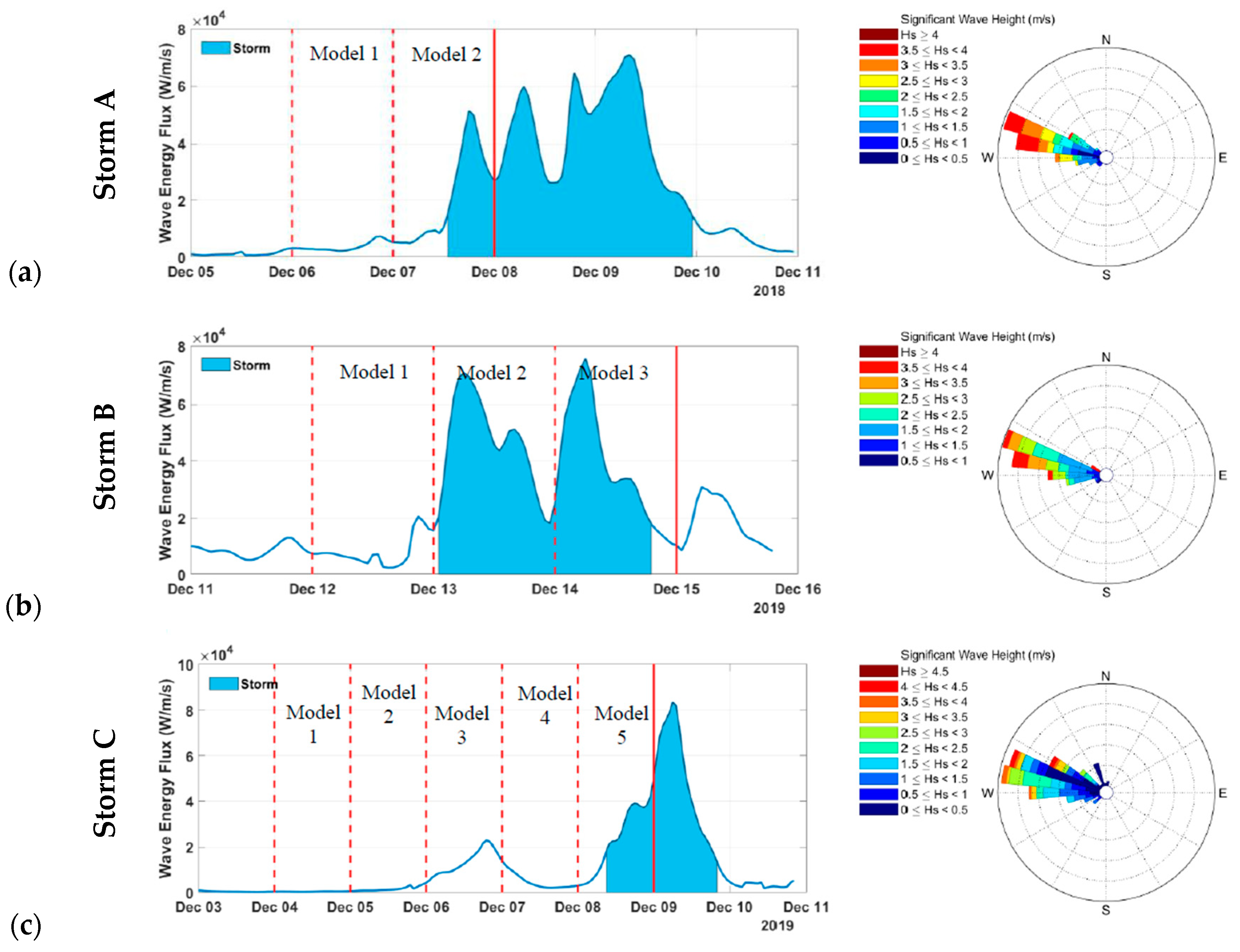
3.2. Hydrodynamic Data and Storm Identification

The hydrodynamic conditions of waves, winds, tides, and surges, close to Etretat, were assessed through a combination of in situ observations and numerical modeling.
The wave data were initially extracted from a wave model [29] as there is no active buoy close to the beaches of Normandy. Waves were then propagated to shore using the SWAN model [33]. Propagation was forced over a total of 26 months, between June 2018 and September 2020, on a regular rectangular grid of 20 m resolution. The model was validated against buoy data near Le Havre (~25 km south to southwest from Etretat) with an RMSE of 0.235 m and a correlation coefficient of 0.927. The time series of wave characteristics used for our XBeach-G models was extracted from the cell where the offshore end of the cross-shore bathymetric transect is located. A more precise description of SWAN model setting is provided in Solano et al. [29].
Astronomical tide, surge, and wind data were extracted from a Hycom2D model [34], built on a curvilinear grid with a resolution of 500 m near the coast. As for the SWAN data, the extraction point is located in the cell where the cross-shore transect ends. Regarding validation, Pasquet et al. [35] reported measuring a tidal phase shift of up to 12 min and an underestimation on the total water level of −10 cm at the peak of storm surges. This shift could induce a possible consequence on the estimation of the morphological elevation during storms. Nevertheless, this remains small compared to the errors generated by in situ measurements and corresponds to less than twice the median grain size.
The winters of 2018–2019 were characterized as the most energetic period in the last decade [36,37,38], causing substantial wave overtopping and seawall damage in Etretat [4] (Figure A1b). Storm events were identified in the hydrodynamic data record using an excessive wave significant height method. Identified storms were sorted according to their total energy. This method is often used to procedurally establish a sorted list of marine storm events [39,40,41]. In the present study, a marine storm was defined as an event during which the significant wave height ( H s ) exceeds a threshold ( H s   t h r e s h o l d ) and lasts for at least 12 h. We introduced H s   t h r e s h o l d as the mean value of H s plus two standard deviations (Equation (1)). In addition, consecutive events separated by an interval of less than 48 h were merged and considered as one longer event [42]. The list of storm events identified includes 30 storms distributed between June 2018 and September 2020. Sorting by decreasing accumulated energy ( E s t o r m , Equation (3)) was then performed. E s t o r m corresponds to the integral of the energy flux ( E f l u x , Equation (2)) over the duration of each event.
H s   t h r e s h o l d = μ H s + 2 σ H s 2
E f l u x t = ϱ g 2 64 π H s 2 T
E s t o r m = t s t o r m   s t a r t t s t o r m   e n d E f l u x t   d t
where ϱ is the sea water density (1025 kg/m3), g is the acceleration of gravity (9.81 m/s2), H s is the wave significant height in meters, and T is the wave period in seconds.
Once sorted, the three storms presenting both high intensity and sufficient bathymetry data were selected (Figure 4). Storm weather conditions tend to decrease the quality of VMS images (water drops, overtopping, depth of field reduced by rain and sea spray). This challenges the identification of an accurate coastline and creates gaps in our time series of intertidal bathymetry during storms. Nevertheless, DEMs could be reconstructed over a total of 11 days, including periods before and during the three selected storms. The selected events correspond to storms A, B, and C; their characteristics are summarized in Table 1. Figure A1a illustrates the wave heights of storm B, with a strong overtopping leading to the flooding of the backshore.
Figure 5 shows the evolution of E f l u x during the 3 selected storm events, as well as the dates on which the intertidal bathymetry data could be measured by the VMS (i.e., start, transition and end dates of the simulations). Only the dates where VMS-derived DEMs were wider than 35 m (an empirically chosen threshold) were considered usable to minimize the potential temporal decorrelation between our profile and the real bathymetry.
Storm A (Figure 5a) consisted of a series of four peaks increasing between 5 × 10⁴ and 7 × 10⁴ W/m/s, of which only the first (i.e., E f l u x = 5 × 10⁴ W/m/s) could be monitored and modeled. Since the calmer period preceding the storm was also covered by one VMS observation, three DEMs were used to simulate two days in using XBeach-G, each model lasting 24 h. Storm B (Figure 5b) consisted of three peaks varying between 5 × 10⁴ and 8 × 10⁴ W/m/s. It is covered from start to finish by four daily intertidal DEMs that allowed three consecutive days of simulation to be computed. Storm C (Figure 5c) consisted of only a single peak where E f l u x = 8 × 10⁴ W/m/s. Unfortunately, only observations prior to the peak are available, although the last available DEM covers the beginning of the event, when E f l u x reached 5 × 10⁴ W/m/s and was intensifying. However, the period preceding this maximum had another peak of lower intensity ( E f l u x = 2 × 10⁴ W/m/s) with a good data temporal coverage. It was, therefore, decided to model this pre-storm period using the 6 DEMs available to simulate 5 days, as bathymetry was updated every 24 h.

3.3. XBeach-G Numerical Setup

XBeach is an open-source numerical model operating in the horizontal plane (2DH), addressing wave propagation, long waves, mean flow, sediment transport, and morphological changes [18]. Two main modes are utilized: nonhydrostatic (XB-NH) for resolving all wave motions (with higher computational expense) and Surfbeat (XB-SB) for resolving wave group scale motions more efficiently. The XB-SB mode, though not resolving sea-swell frequency motions, computes steady setup, (un)steady currents, and infra-gravity wave motions, especially relevant in dissipative events and fringing reef environments. XB-NH calculates depth-averaged flow due to waves and currents using non-linear shallow water equations, incorporating a nonhydrostatic pressure correction akin to a one-layer SWASH model.
The development of XBeach-G, a one-dimensional extension of XBeach dedicated to gravel barriers, was incentivized by the diverging results of XBeach when applied to gravel systems, suggesting that physical forcings needed to be considered differently in such contexts [19]. XBeach-G uses the NH mode to solve the non-linear shallow water equations (NLSWE) and calculate the depth-averaged flow due to waves and currents, taking groundwater exchange into account (Equation (4)).
δ ζ δ t + δ h u δ x + S = 0 δ u δ t + u δ u δ x δ δ x ν h δ u δ x = 1 ρ ρ q ¯ + ρ g ζ δ x τ b ρ h
where t and x represent the temporal and spatial (horizontal) coordinates, respectively, ζ is the elevation of the free surface, h is the water depth, u is the depth-averaged cross-shore velocity, S is the exchange flux between surface water and groundwater (proportional to the permeability k ), ν h is the water viscosity (horizontal), ρ is the water density, q ¯ is the depth-averaged dynamic pressure (normalized by the water density), g is the acceleration due to gravity, and τ b is the bed shear stress.
The aim of the present numerical investigation is to assess beach permeability evolution by modeling storms with varying permeability ( k ) within the range of 0 to 0.6 m/s. This range aligns with the expected permeability for the measured surficial grain size in Etretat [7,43,44]. Storms are segmented and modeled in 24 h intervals, approximately matching the daily frequency of intertidal bathymetry estimation from VMS observations.
The 3500 m long bathymetric profile (Figure 6a) is distributed on a 1D mesh of 1232 nodes with a variable spacing ranging between 3 m offshore and 1 m close to the beach. An empirically defined non-erodible layer immobilizes sections corresponding to the seawall and below elevation −6 m (Figure 6b) and the hardground bedrock. The seawall profile is defined as a vertical plane extending from −6 m to +9 m, although it is most likely an inclined plane (the precise morphology of the seawall below the sediment is unknown). Thus, only the section of the profile between −6 and +9 m in elevation is composed of material that can be mobilized by waves, although sediment could theoretically be deposited and then removed outside these limits, depending on hydrodynamic conditions.
A sensitivity analysis on permeability k involves running 10 to 13 model scenarios for each modeled day. Three metrics—the root mean square error (RMSE, Equation (5)) between measured and modeled profiles, the coefficient of determination (R2, Equation (6)) on the relative change in elevation, and the Brier Skill Score ( B S S , Equation (7))—are computed to evaluate model performance, focusing on the intertidal zone where VMS-derived elevation data are available.
R M S E = z z 2  
where z is the observed elevation along the profile, and z is the modeled one.
R = C o v X , Y σ X × σ Y
where C o v X , Y is the covariance between two vectors X and Y , as calculated by C o v X , Y = E X X ¯ × Y Y ¯ .
The equation of B S S considers the initial observed and both final observed and modeled profiles. The main advantage of this index is that it only takes into account the active part of the profile [45], thus limiting potential bias such as the presence of a non-erodible profile section. B S S values are generally considered good for values superior to 0.6; Table 2 provides an interpretation chart based on the work of Van Rijn et al. [46].
B S S = 1 1 N i = 1 N z f i n a l ,   i z f i n a l ,   i 2 1 N i = 1 N z i n i t i a l ,   i z f i n a l ,   i 2
The cross-shore profile starts offshore at a depth of 24.6 m and extends 3490 m up to the seawall at +9 m. Resolution is gradually refined from 3 m offshore to 1 m near the seawall to capture wave processes adequately. The selected transect minimizes alongshore transport effects, which are not considered by XBeach-G, due to its location around the beach cell rotation pivot center, despite significant transport demonstrated by shoreline rotation mechanisms [4].

4. Results

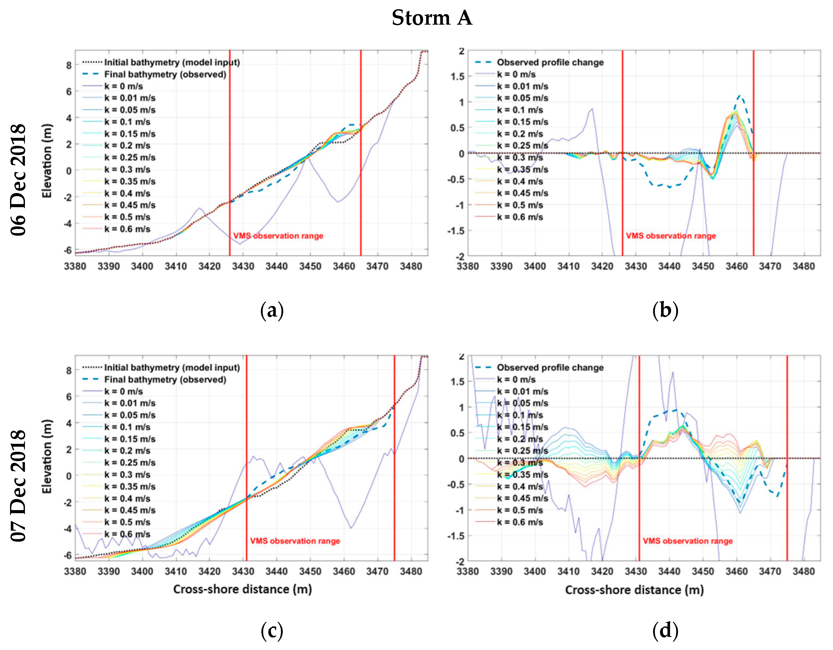
4.1. XBeach-G Storm Simulations

The morphological response of the intertidal topography was numerically investigated for three distinct storm events (A, B, and C), each characterized by different severity and duration. The validity of these investigations was established through video observations, utilized for calibrating the initial profile extracted before each event.
Numerical simulations of the selected beach profile were conducted for thirteen permeability values, ranging from 0 to 0.6, during each storm event (A, B, and C). For each storm, XBeach-G simulations were performed every 24 h (twice for storm A over 35 h, 3 times for storm B over 42 h, and 5 times for storm C over 58 h), resulting in a total of 26, 39, and 56 numerical simulations for storms A, B, and C, respectively. Selected simulations are illustrated in Figure 7, Figure A2 and Figure A3. Subsequently, error calculations were performed for each simulation, encompassing varying permeability values and time intervals corresponding to the progression of storms, with assessments conducted every 24 h.
Table 3 presents a summary of BSS, RMSE, and R2 results for various permeability scenarios during storm A. Further results of storms B and C are presented in Table A1. Among the modeled dates, only four achieved BSS values higher than 0.3 (threshold of the “fair” category Van Rijn et al. [46]), with two exceeding 0.6 (“good” category). The highest BSS values occurred during the most intense storm (storm A), particularly during the peak between 07 Dec 2018 and 08 Dec 2018 ( E f l u x   m a x = 7.1 × 10⁴ W/m/s). However, storm B, with a higher-intensity peak ( E f l u x   m a x = 7.5 × 10⁴ W/m/s), did not yield BSS values above 0.3, indicating no clear correlation between BSS and wave condition intensity. The lowest BSS values were associated with permeability value k = 0, equivalent to the deactivation of the groundwater flow process.
BSS values covaried with permeability, suggesting that the maximum BSS value for one date indicates the optimal permeability value. Two consecutive dates with BSS exceeding 0.6 were identified: on 16 Dec 2018, optimal k was between 0.2 and 0.35 m/s under relatively calm conditions ( E f l u x   m a x = 5 × 10³ W/m/s), and on 07 Dec 2018, optimal k ranged between 0.01 and 0.15 m/s (maximum for k = 0.01 m/s) during a storm peak ( E f l u x   m a x = 5 × 10⁴ W/m/s). Both dates exhibited a minimum RMSE of 0.26 m and maximum R2 of 0.73 and 0.75, respectively.
The two dates with BSS classified as “fair” (13 Dec 2019, BSS = 0.33, and 05 Dec 2019, BSS = 0.32) remained in the lower limit (0.3) of the fair class. These dates corresponded to storm conditions ( E f l u x   m a x = 7 × 10⁴ W/m/s) and calm conditions ( E f l u x   m a x = 1 × 10² W/m/s), respectively, with associated RMSE values of 0.49 m and 0.11 m, and R2 of 0.07 and 0.57. Results from the XBeach-G model were more significant for the storm A compared to storms B and C (Table 3 and Table A1).
Detailed analysis of the intertidal profile changes on 06 Dec 2019 revealed the accurate reproduction of accretion phenomena at the top of the beach for various permeability values. However, simulated movements in the lower part of the beach were underestimated, particularly with lower permeability values, excluding k = 0 m/s. On 07 Dec 2019, where hydrodynamic conditions were stronger, the model accurately reproduced accretion at the bottom of the beach for different k values, indicating lower sensitivity to permeability. However, erosion of the upper beach was only reproduced for low k values. Notably, for permeability values exceeding 0.3 m/s, the model predicted accretion of the upper beach instead of erosion, highlighting greater sensitivity to permeability in this region of the profile. The scenario with k = 0 m/s significantly overestimated both lower-beach accretion and upper-beach erosion. Modeled movements outside the area monitored by VMS remained relatively small.

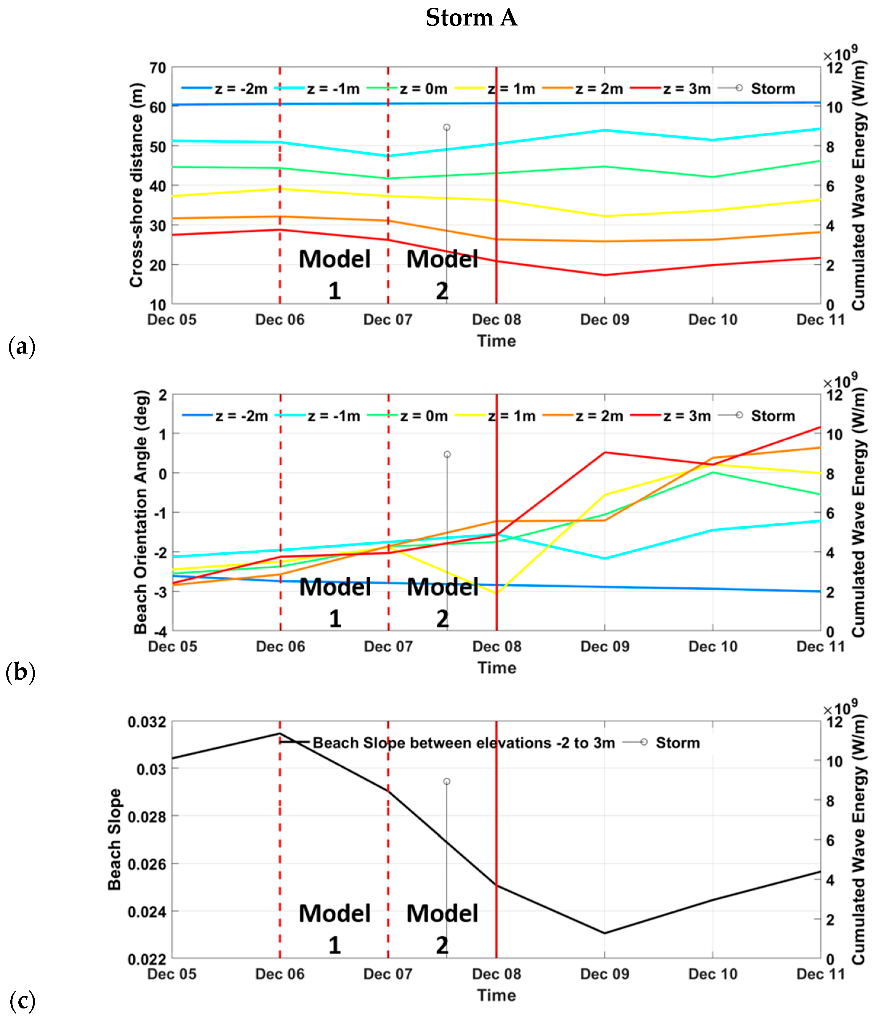
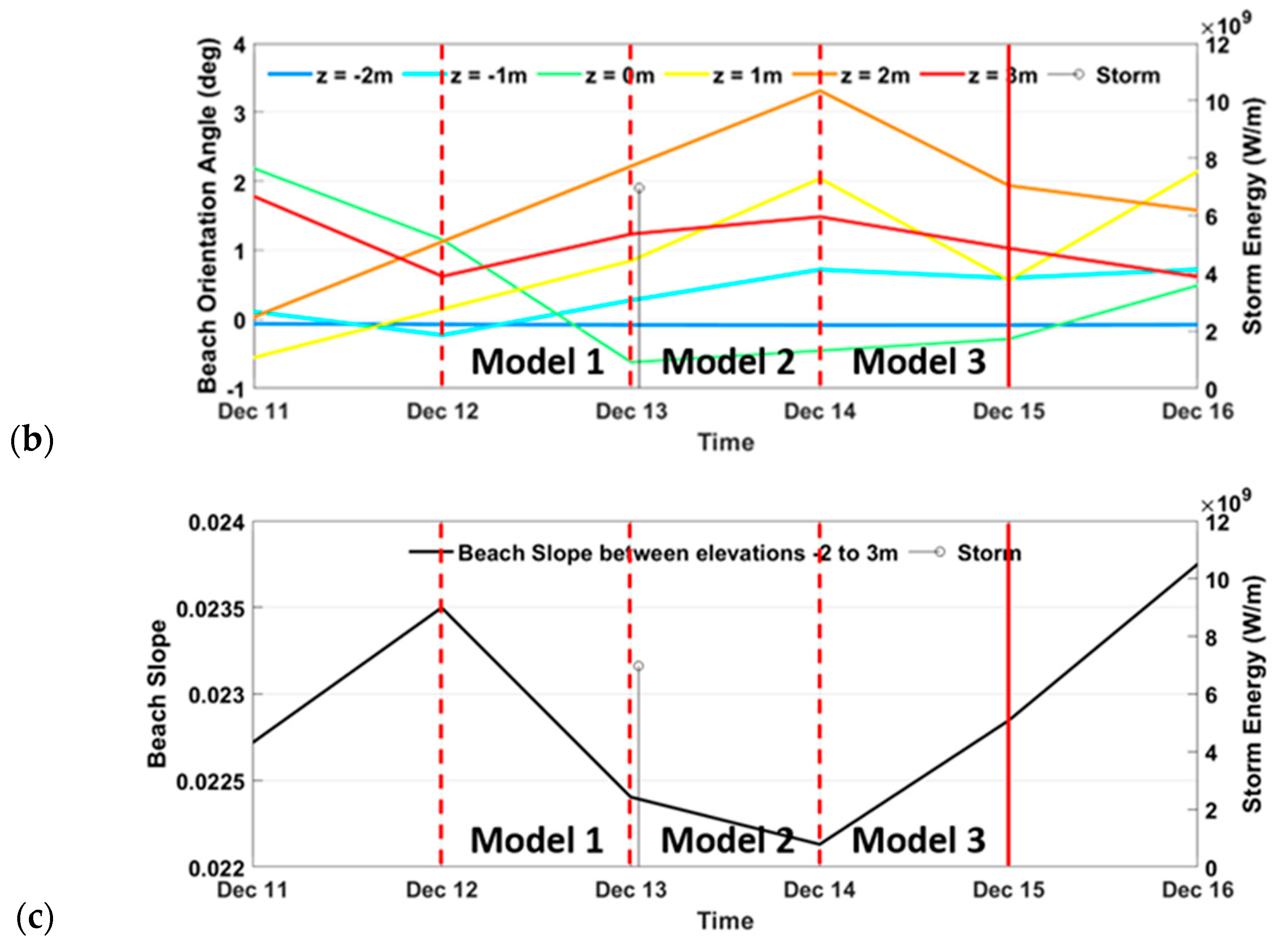
4.2. Morphological Observations

Three indices of morphological variability on the beach in response to the different storm events were extracted from the VMS-derived DEMs (Figure 8). The beach width (BW) was estimated as the average horizontal distance separating the DEM’s contour lines of various elevations from −2 m to 3 m. The beach slope (BS) was computed as the ratio between the tidal range and BW. The beach orientation is calculated by approximating the shoreline to a parabola. The orientation angle (BOA) is then calculated as the angle between the seawall and the parabola’s tangent at the transect location (Figure 3b). The results are presented in Figure 8 for storm A, and Figure A2 and Figure A3 for storms B and C, respectively.

5. Discussion

5.1. Influence of Permeability on Morphodynamics

During storm A, the results highlight the sensitivity of pebble beach morphodynamics to permeability. The absence of groundwater flow ( k = 0 m/s) exaggerates sediment erosion and accumulation phenomena significantly, emphasizing the crucial role of considering groundwater flow in estimating these dynamics. This is consistent with observations from Buscombe and Masselink [43], Jennings and Shulmeister [27], and Mason and Coates [47], and was one of the main incentives for the adaptation of XBeach for gravel environments [7]. This sensitivity is explained by the importance of water seepage in the rapid loss of wave energy during uprush on gravel beaches.
Generally, the results show that for non-zero values, k controls the amplitude of the profile changes, while the position along the profile of the maximum and minimum changes depends on the antecedent topography and hydrodynamic conditions (tidal amplitude, wave characteristics). Lower k values in calm conditions tend to smoothen the profile, while higher k values favor berm buildup in the upper intertidal zone. Under energetic conditions, low permeability fosters profile erosion and accumulation at the beach step, while high values tend to build a berm by eroding the beach step. This aligns with findings by She et al. [48], who observed increased offshore sediment transport and reduced onshore transport with decreasing permeability in a mixed sand and gravel beach physical model.

5.2. Limitations of the Modelling Approach

The low number of models meeting the BSS ≥ 0.6 condition underscores the limitations of the approach. Challenges include the reduced quality of VMS images in winter conditions, especially during storms, which affects the reconstruction of DEMs in terms of number, extension, and potentially quality. Additionally, the model updates only the intertidal section of the profile visible to cameras from one storm to the next, neglecting potential subtidal changes and features like the beach step, known for its importance in gravel beach dynamics [43,49,50]. Similarly, supratidal morphology, constituting a sedimentary stock accessible to storm overtopping waves, is not updated. Despite these limitations, the model results for storm 2 align well with observed morphological changes, suggesting relative closeness to reality for that specific date.
Other studies at different sites reveal similar model performances. For example, Pollard [51] modeled the storm response of a gravel barrier in the UK, where the D50 varied between 1 and 2 cm. Forty-five calibration runs, including permeability variations, yielded a maximum BSS of 0.71 for k = 0.2 m/s. The model was then applied to seven different profiles, among which only two resulted in BSS values greater than 0.6. Bergillos et al. [22] applied XBeach-G to a mixed sand and gravel deltaic coastline with a D50 of 2 cm. Permeability was not reported by the authors, but their results show BSS values greater than 0.89. Brown et al. [23] tested the model on a mixed sand and gravel beach in New Zealand, with a D50 of 1.36 cm and a permeability k = 0.01 m/s. Only 7 of the 30 scenarios obtained a BSS greater than 0.6, with a maximum of 0.79.

5.3. Implications of Grain Size for Modelling Pebble Beaches

The observed morphological changes during the calm period involve the construction of a horizontal berm, while the initial peak of storm A results in berm erosion and profile smoothing. These behaviors align with findings by McCall et al. [20] and correspond to the rollover mechanism [4]. McCall et al. [20] defined rollover as the cross-shore landward displacement of the entire profile of a barrier without a change in height, width, or slope. Although the beach of Etretat is not precisely a barrier due to its fixed seawall constraint, the rollover manifests as an oscillation of the slope around a pivot axis in the system at the x = 3450 m coordinate and between 0 and +1 m in elevation (Figure 7 and Figure 8a,c).
Furthermore, the position along the profile and the width of the horizontal berms vary from one date to another and appear to be correlated with the permeability value and the intensity of hydrodynamic conditions. Specifically, for any given date, a larger k value tends to shape the berm, while a lower k value is likely to erase it and smoothen the profile shape (Figure 7, Figure A2 and Figure A3). The study of the morphological characteristics of berms as a proxy for permeability during storms emerges as a relevant research axis for future investigations.
Considering a well-sorted sediment, a larger sediment size implies a grater porosity and increased seepage velocities under swash (i.e., an enhanced ability to dissipate wave energy) [43]. The observed significant granulometric sorting on gravel beaches with strong spatial and temporal variability [4,43], as well as the mobilization of a substantial amount of sediment during storm events [52], suggests that the permeability of a beach may vary on a daily scale. In the case of a gravel beach, it is reasonable to expect greater permeability during sustained calm conditions over a longer period, allowing finer sediments to migrate through the porosity. Conversely, under more energetic conditions, the sudden mobilization of sediment can mix grain sizes and potentially decrease permeability.
Indeed, studies on mixed gravel and sand beaches highlight that the presence of sand plays a crucial role in influencing the response of the beach profile to wave impact. Permeability, in such cases, is controlled by the finest 10% of the sediment [53,54]. Mason et al. [55] demonstrated that when the surface sedimentary layer (depth < 1 m) contains more than 25% of its weight in sand, the beach morphodynamics become more similar to that of sandy beaches than mixed ones.
Although Etretat is primarily considered a pebble, there exists a significant amount of underlying sand in the system. In certain instances, after storms, this sand can become the predominant substrate of the beach. While this occurrence is rare, it demonstrates that finer materials, such as sand, could fill up the pebble’s porosity and potentially reduce the permeability of the beach.
Under this hypothesis, the impact of successive storms of moderate intensity in a cluster could be greater than stronger but isolated events. This is because clustered storms would occur on a beach with a permeability lowered by antecedent storms, hence with a reduced ability to absorb wave energy through infiltration/exfiltration processes.
Storm A was preceded by a month of calm conditions, with the previous storm occurring on November 8. Before the first peak of storm A, the model results indicate that the permeability optimum was between 0.20 and 0.35 m/s in calm conditions, later reduced to around 0.05 m/s under more energetic conditions. These values approximately correspond to well-sorted coarse and fine gravel sizes, respectively [43,56]. These results suggest strong and rapid temporal variability in permeability in pebble systems, with a decrease by a factor of 4 at least within a day.
The strict character, “purely gravel”, of the beach (the word gravel is here referring to particles coarser than 2 mm, i.e., sand) could shift occasionally to a “mixed sand and gravel”-type system. Considering that storms are seasonal events, the transition from pure gravel to mixed sand and gravel behavior (i.e., not necessarily resulting in surficial sand) could be seasonal as well. An analogous seasonal transition between beach types was documented by Casamayor et al. [56] on a composite beach. The authors found that their composite study site behaved as a pure gravel system in winter and as a composite system during summer due to wave climate variability and associated morphological changes. They proposed adding a seasonal component to the composite beach type of Jennings and Shulmeister [27], and the results here tend to support that it could be a relevant addition for the pure gravel type as well.
Moreover, the low BSS results obtained with models of storms B and C could be partly due to the beach behaving more like a sandy one. In such cases, the sediment transport equations used by XBeach-G could become obsolete, highlighting the need for a more nuanced understanding of the beach composition and dynamics in different seasonal and storm contexts.
This analysis provides valuable insights into the complex interplay between storm dynamics, permeability, and morphological changes in pebble beaches, highlighting the need for further exploration in this field.

5.4. Insights on the Complex Evolution of Pebble Beaches

In summary, it was possible to successfully model a portion of storm A in Etretat, despite the inherent limitations of the dataset. However, the modeling capabilities remain limited by the previously mentioned data accuracy limitations and by the conceptual simplifications of Xbeach-G. The reliance on 1D model computations leads to ignoring potentially important longshore exchanges (Soloy et al., [4], especially in the case of an oblique storm swell such as in Etretat. Notably, storm A stood out as the only modeled event where BOA remained consistently aligned at all elevations (from −2 to −3 degrees), with only 1 degree of clockwise rotation during the modeled period. Conversely, other storms exhibited broader variations in shoreline orientations (Figure A4 and Figure A5), pointing to localized alongshore processes introducing significant complexity not accounted for in Xbeach-G.
The findings also underscore notable daily variability in permeability, aligning with recent observations on the spatiotemporal variability in the surface grain size of pebble beaches. However, k is imposed as a spatially and temporally uniform constant, due to the inherent challenges in accurately measuring this parameter, which may limit model convergence and, by extension, the ability to model gravel coasts. Moreover, although gravel size strongly influences permeability and is known to vary over time and space (Horn and Walton, [54]), it is described in Xbeach as spatially and temporally uniform, relying on single values of D50 and D90. Advancements in coastal monitoring and grain size mapping techniques proposed in recent studies [17,26] hold the promise of providing high-resolution observational datasets. Utilizing such data could significantly enhance models, enabling a more accurate consideration of the spatiotemporal variability in permeability during storm events.

6. Conclusions

This study employed Xbeach-G to simulate the impact of three intense storms occurring between 2018 and 2020 on the Etretat beach in Normandy, France. The modeling aimed to calibrate the permeability value (k) to understand its day-to-day and inter-storm variations. Among the modeled events, satisfactory results were obtained for storm A, with maximum BSS values of 0.63 and 0.69 on the first and second modeled days, respectively. These results indicated permeability values of k = 0.20 m/s to 0.35 m/s and k = 0.05 m/s, consistent with expectations for well-sorted coarse and fine gravel sizes, respectively.
However, storms B and C yielded unsatisfactory results, likely due to limitations in the approach, including imprecise subtidal and supratidal topography, lack of updating in the subtidal area, and the neglect of longshore sediment transport. Indeed, the time series of beach orientation angle suggested significant longshore transport, which the model could not capture due to the one-dimensional nature of Xbeach-G.
This study emphasized the sensitivity of the beach profile to permeability, where high values led to berm formation, and low values resulted in erosion. The intensity of wave conditions influenced the amplitude of topographic changes. The storm A results indicated a potential fourfold decrease in permeability within 24 h, emphasizing the dynamic nature of pebble beaches during storm events, especially regarding their ability to dissipate wave energy through infiltration/exfiltration processes.
The findings challenged the strict characterization of Etretat’s beach as “purely gravel”, suggesting occasional transitions to a “mixed sand and gravel” system, possibly seasonal. The spatial and temporal uniformity of k, grain size, and porosity were identified as limitations in the Xbeach-G model. Future developments could involve incorporating granulometric observations and addressing these limitations for a more accurate representation of gravelly systems. This study underscores the complexity of pebble beaches, advocating for innovative techniques, model improvements, and integrative approaches, combining numerical models, physical experiments, and field observations to enhance the understanding of morphological responses and uncertainties.

Author Contributions

Conceptualization, A.S., E.I.T. and N.L.; methodology, A.S., E.I.T. and N.L.; software, A.S. and C.L.S.; validation, A.S.; formal analysis, A.S., E.I.T. and N.L.; investigation, A.S., E.I.T. and N.L.; resources, A.S., E.I.T., N.L. and C.L.S.; data curation, A.S. and C.L.S.; writing—original draft preparation, A.S. and E.I.T.; writing—review and editing, A.S., E.I.T., N.L., E.T.M. and C.L.S.; visualization, A.S.; supervision, E.I.T. and N.L.; project administration, E.I.T. and N.L.; funding acquisition, E.I.T. and N.L. All authors have read and agreed to the published version of the manuscript.

Funding

This research received no external funding.

Data Availability Statement

The data used in this paper are accessible upon request by email to the corresponding author.

Acknowledgments

The authors wish to thank the city services of Etretat as well as the Seine-Maritime Departmental Council and the Normandy Region for supporting the monitoring of the beach and enhancing the scientific activities along Normandy coasts; Additionally, the authors would like to thank, SHOM and Waves’n See company (co-founder Yves Soufflet) for the technical support and the management of the video monitoring systems. This work used the outcomes of several activities carried out in the framework of two research programs.

Conflicts of Interest

The authors declare no conflicts of interest.

Appendix A

Figure A1. Seawall damages in Etretat on 12 Mar 2019 after high-energy conditions (a); damage to Etretat’s seawall after a storm in early 2020 (b).
Jmse 12 00327 g0a1
Table A1. Validation results of the XBeach-G simulations of both storms B and C. Metrics include the Brier Skill Score (BSS), the root mean square error (RMSE) and the coefficient of determination (R2). Red values in bold highlight scenarios with BSS > 0.6, RMSE < 0.25 m, or R2 > 0.9. Yellow values in italic indicate BSS > 0.3, RMSE < 0.5 or R2 > 0.5.
ParameterStormDatesk (m/s)
00.010.050.10.150.20.250.30.350.40.450.50.6
BSSB12 Dec 2019−12.54−0.53−0.48−0.48−0.50−0.48−0.50−0.49−0.50−0.48−0.48−0.47−0.44
13 Dec 2019−76.51−0.68−0.53−0.41−0.31−0.20−0.13−0.040.050.120.210.220.33
14 Dec 2019−12.68−3.03−2.75−2.55−2.42−2.29−2.20−2.13−2.04−1.93−1.87−1.78−1.55
C04 Dec 2019-−0.05−0.19−0.33−0.41−0.49−0.52−0.52−0.52−0.51--−0.37
05 Dec 2019-0.320.14−0.07−0.23−0.37−0.51−0.59−0.66−0.64--−0.51
06 Dec 2019-−1.69−2.12−2.52−2.85−3.17−3.45−3.74−3.95−4.10--−4.11
07 Dec 2019-−0.30−0.41−0.49−0.55−0.58−0.59−0.60−0.56−0.55--−0.41
08 Dec 2019-0.290.08−0.14−0.40−0.67−0.94−1.21−1.47−1.72--−2.56
RMSEB12 Dec 20192.740.900.870.870.880.890.900.900.910.900.910.900.90
13 Dec 20195.650.780.750.730.700.680.650.620.590.560.530.530.49
14 Dec 20191.400.810.800.780.770.760.750.740.720.710.700.680.64
C04 Dec 2019-0.220.230.240.240.250.250.250.240.24--0.23
05 Dec 2019-0.110.130.140.150.150.160.170.170.17--0.16
06 Dec 2019-0.400.430.460.480.490.510.520.530.53--0.52
07 Dec 2019-0.350.370.380.390.400.390.390.380.38--0.34
08 Dec 2019-0.440.480.530.590.650.700.750.790.83--0.97
R2B12 Dec 20190.680.240.180.140.100.070.050.030.020.000.000.000.00
13 Dec 20190.240.020.020.010.010.010.000.000.000.010.030.030.07
14 Dec 20190.010.090.070.060.050.040.040.030.030.020.010.010.01
C04 Dec 2019-0.020.130.190.190.200.200.190.180.17--0.11
05 Dec 2019-0.570.590.590.590.590.570.550.530.52--0.42
06 Dec 2019-0.110.130.130.140.140.150.170.190.19--0.17
07 Dec 2019-0.470.550.600.640.620.580.530.480.45--0.19
08 Dec 2019-0.560.450.350.250.180.110.070.040.02--0.00
Figure A2. Numerical simulations of the beach response for storm B. Comparison between observed (black dotted and blue dashed lines) and modeled cross-shore profiles of Etretat using Xbeach-G (colored solid lines, one color per value of permeability k). (af) present results after one day of observation/modeling during storm B (12 Dec 2019 to 15 Dec 2019). The initial and final profiles are presented in (a,c,e) while the associated elevation change is presented in (b,d,f). The red vertical lines present the extent of the area monitored daily through video monitoring system (i.e., the section of the profile that was observed at the model’s beginning and ending dates).
Jmse 12 00327 g0a2aJmse 12 00327 g0a2b
Figure A3. Numerical simulations of the beach response for the storm C. Comparison between observed (black dotted and blue dashed lines) and modeled cross-shore profiles of Etretat using Xbeach-G (colored solid lines, one color per value of permeability k). (aj) present results after one day of observation/modeling during storm B (04 Dec 2019 to 09 Dec 2019). The initial and final profiles are presented in (a,c,e,g,i) while the associated elevation change is presented in (b,d,f,h,j).The red vertical lines present the extent of the area monitored daily through video monitoring system (i.e., the section of the profile that was observed at the model’s beginning and ending dates).
Jmse 12 00327 g0a3aJmse 12 00327 g0a3b
Figure A4. Beach response to storm B from video observations (VMS) compared to numerical simulations. Beach width (BW, (a)), beach orientation angle (BOA, (b)) and beach slope (BS, (c)) observed using VMS during storm B, at various elevations from −2 m to +3 m. The storm starting date is presented as a vertical bar, its height relates to the cumulated wave energy. Vertical red lines (both dashed and solid) indicate the dates at which VMS-derived intertidal DEMs were available, the dashed ones specifically correspond to model starting dates while the solid lines indicate the last date with data available for model performance assessment.
Jmse 12 00327 g0a4aJmse 12 00327 g0a4b
Figure A5. Beach response to storm C from video observations (VMS) compared to numerical simulations. Beach width (BW, (a)), beach orientation angle (BOA, (b)) and beach slope (BS, (c)) observed using VMS during storm 7, at various elevations from −2 m to +3 m. The storm starting date is presented as a vertical bar, its height relates to the cumulated wave energy. Vertical red lines (both dashed and solid) indicate the dates at which VMS-derived intertidal DEMs were available, the dashed ones specifically correspond to model starting dates while the solid lines indicate the last date with data available for model performance assessment.
Jmse 12 00327 g0a5aJmse 12 00327 g0a5b

References

  1. Carter, R.W.G.; Orford, J.D. The Morphodynamics of Coarse Clastic Beaches and Barriers: A Short- and Long-term Perspective. Source J. Coast. Res. 1993, 15, 158–179. [Google Scholar]
  2. Buscombe, D.; Masselink, G. Grain-size information from the statistical properties of digital images of sediment. Sedimentology 2009, 56, 421–438. [Google Scholar] [CrossRef]
  3. Almeida, L.P.; Masselink, G.; Russell, P.E.; Davidson, M.A. Observations of gravel beach dynamics during high energy wave conditions using a laser scanner. Geomorphology 2015, 228, 15–27. [Google Scholar] [CrossRef]
  4. Soloy, A.; Turki, I.; Lecoq, N.; Solano, C.L.; Laignel, B. Spatio-temporal variability of the morpho-sedimentary dynamics observed on two gravel beaches in response to hydrodynamic forcing. Mar. Geol. 2022, 447, 106796. [Google Scholar] [CrossRef]
  5. Ions, K.; Karunarathna, H.; Reeve, D.E.; Pender, D. Gravel barrier beach morphodynamic response to extreme conditions. J. Mar. Sci. Eng. 2021, 9, 135. [Google Scholar] [CrossRef]
  6. Jamal, M.H.; Simmonds, D.J.; Magar, V. Modelling gravel beach dynamics with XBeach. Coast. Eng. 2014, 89, 20–29. [Google Scholar] [CrossRef]
  7. McCall, R.T. Process-Based Modelling of Storm Impacts on Gravel Coasts; University of Plymouth: Plymouth, UK, 2015. [Google Scholar]
  8. Powell, K.A. Predicting Short Term Profile Response for Shingle Beaches; Hydraulics Research Wallingford: Wallingford, UK, 1990. [Google Scholar]
  9. Bradbury, A.P.; Cope, S.N.; Prouty, D.B. Predicting the Response of Shingle Barrier Beaches under Extreme Wave and Water Level Conditions in Southern England. In Coastal Dynamics 2005—Proceedings of the Fifth Coastal Dynamics International Conference, Barcelona, Spain, 4–8 April 2005; American Society of Civil Engineers: Reston, VA, USA, 2006; pp. 1–14. [Google Scholar] [CrossRef]
  10. Bradbury, A.P.; Powell, K.A. The short term profile response of shingle spits to storm wave action. In Coastal Engineering 1992: Proceedings of the Twenty-Third International Conference, Venice, Italy, 4–9 October 1992; American Society of Civil Engineers: Reston, VA, USA, 1993; pp. 2694–2707. [Google Scholar]
  11. Almeida, L.P.; Masselink, G.; Russell, P.; Davidson, M.; Poate, T.; McCall, R.; Blenkinsopp, C.; Turner, I. Observations of the swash zone on a gravel beach during a storm using a laser-scanner (Lidar). J. Coast. Res. 2013, 65, 636–641. [Google Scholar] [CrossRef]
  12. Simarro, G.; Calvete, D.; Souto, P. UCalib: Cameras Autocalibration on Coastal Video Monitoring Systems. Remote Sens. 2021, 13, 2795. [Google Scholar] [CrossRef]
  13. Nieto, M.A.; Garau, B.; Balle, S.; Simarro, G.; Zarruk, G.A.; Ortiz, A.; Tintoré, J.; Álvarez-Ellacuría, A.; Gómez-Pujol, L.; Orfila, A. An open source, low cost video-based coastal monitoring system. Earth Surf. Process. Landforms 2010, 35, 1712–1719. [Google Scholar] [CrossRef]
  14. Andriolo, U. Nearshore Hydrodynamics and Morphology Derived from Video Imagery; Universidade de Lisboa: Lisbon, Portugal, 2018. [Google Scholar]
  15. Vousdoukas, M.I.; Ferreira, P.M.; Almeida, L.P.; Dodet, G.; Psaros, F.; Andriolo, U.; Taborda, R.; Silva, A.N.; Ruano, A.; Ferreira, Ó.M. Performance of intertidal topography video monitoring of a meso-tidal reflective beach in South Portugal. Ocean Dyn. 2011, 61, 1521–1540. [Google Scholar] [CrossRef]
  16. Arriaga, J.; Medellin, G.; Ojeda, E.; Salles, P. Shoreline Detection Accuracy from Video Monitoring Systems. J. Mar. Sci. Eng. 2022, 10, 95. [Google Scholar] [CrossRef]
  17. Soloy, A.; Turki, I.; Lecoq, N.; Gutiérrez Barceló, Á.D.; Costa, S.; Laignel, B.; Bazin, B.; Soufflet, Y.; Le Louargant, L.; Maquaire, O. A fully automated method for monitoring the intertidal topography using Video Monitoring Systems. Coast. Eng. 2021, 167, 103894. [Google Scholar] [CrossRef]
  18. Roelvink, D.; Reniers, A.; van Dongeren, A.; van Thiel de Vries, J.; McCall, R.; Lescinski, J. Modelling storm impacts on beaches, dunes and barrier islands. Coast. Eng. 2009, 56, 1133–1152. [Google Scholar] [CrossRef]
  19. Masselink, G.; Poate, T.; McCall, R.; van Geer, P. Modelling storm response on gravel beaches using XBeach-G. Proc. Inst. Civ. Eng. Marit. Eng. 2014, 167, 173–191. [Google Scholar] [CrossRef]
  20. McCall, R.T.; Masselink, G.; Poate, T.G.; Roelvink, J.A.; Almeida, L.P. Modelling the morphodynamics of gravel beaches during storms with XBeach-G. Coast. Eng. 2015, 103, 52–66. [Google Scholar] [CrossRef]
  21. Almeida, L.P.; Masselink, G.; McCall, R.; Russell, P. Storm overwash of a gravel barrier: Field measurements and XBeach-G modelling. Coast. Eng. 2017, 120, 22–35. [Google Scholar] [CrossRef]
  22. Bergillos, R.J.; Masselink, G.; McCall, R.T.; Ortega-Sánchez, M. Modelling overwash vulnerability along mixed sand-gravel coasts with XBeach-G: Case study of Playa Granada, southern Spain. Coast. Eng. Proc. 2016, 1, 13. [Google Scholar]
  23. Brown, S.I.; Dickson, M.E.; Kench, P.S.; Bergillos, R.J. Modelling gravel barrier response to storms and sudden relative sea-level change using XBeach-G. Mar. Geol. 2019, 410, 164–175. [Google Scholar] [CrossRef]
  24. Ketteridge, K.E.; Cote, J.; Sanderson, T. Predicting storm impacts on gravel beaches in Puget Sound using the XBeach-G model. In Proceedings of the Salish Sea Ecosystem Conference, Seattle, WA, USA, 4–6 April 2018. [Google Scholar]
  25. Costa, S.; Maquaire, O.; Letortu, P.; Thirard, G.; Compain, V.; Roulland, T.; Medjkane, M.; Davidson, R.; Graff, K.; Lissak, C.; et al. Sedimentary Coastal Cliffs of Normandy: Modalities and Quantification of Retreat. J. Coast. Res. 2019, 88, 46–60. [Google Scholar] [CrossRef]
  26. Soloy, A.; Turki, I.; Fournier, M.; Costa, S.; Peuziat, B.; Lecoq, N. A deep learning-based method for quantifying and mapping the grain size on pebble beaches. Remote Sens. 2020, 12, 3659. [Google Scholar] [CrossRef]
  27. Jennings, R.; Shulmeister, J. A field based classification scheme for gravel beaches. Mar. Geol. 2002, 186, 211–228. [Google Scholar] [CrossRef]
  28. Levoy, F.; Anthony, E.J.; Monfort, O.; Larsonneur, C. The morphodynamics of megatidal beaches in Normandy, France. Mar. Geol. 2000, 171, 39–59. [Google Scholar] [CrossRef]
  29. Solano, C.L.; Turki, E.I.; Hamdi, Y.; Soloy, A.; Costa, S.; Laignel, B.; Barceló, Á.D.G.; Abcha, N.; Jacono, D.; Lafite, R. Dynamics of Nearshore Waves during Storms: Case of the English Channel and the Normandy Coasts. Water 2022, 14, 321. [Google Scholar] [CrossRef]
  30. SHOM. MNT Bathymétrique de Façade Atlantique (Projet Homonim). 2015. Available online: https://geo.data.gouv.fr/fr/ (accessed on 20 September 2021).
  31. ROL Réseau D’observation du Littoral de Normandie et des Hauts-de-France. Available online: www.rolnp.fr (accessed on 20 September 2021).
  32. Costa, S.; Letortu, P.; Laignel, B. The hydro-sedimentary system of the upper-normandy coast: Synthesis. In Sediment Fluxes in Coastal Areas; Springer: Berlin/Heidelberg, Germany, 2015; pp. 121–147. [Google Scholar]
  33. Booij, N.; Ris, R.C.; Holthuijsen, L.H. A third-generation wave model for coastal regions: 1. Model description and validation. J. Geophys. Res. Ocean. 1999, 104, 7649–7666. [Google Scholar] [CrossRef]
  34. Chassignet, E.P.; Hurlburt, H.E.; Smedstad, O.M.; Halliwell, G.R.; Hogan, P.J.; Wallcraft, A.J.; Baraille, R.; Bleck, R. The HYCOM (HYbrid Coordinate Ocean Model) data assimilative system. J. Mar. Syst. 2007, 65, 60–83. [Google Scholar] [CrossRef]
  35. Turki, I.; Massei, N.; Laignel, B. Linking sea level dynamic and exceptional events to large-scale atmospheric circulation variability: A case of the Seine Bay, France. Oceanologia 2019, 61, 321–330. [Google Scholar] [CrossRef]
  36. Turki, I.; Massei, N.; Laignel, B.; Shafiei, H. Effects of global climate oscillations on Intermonthly to interannual variability of sea levels along the English channel coasts (NW France). Oceanologia 2020, 62, 226–242. [Google Scholar] [CrossRef]
  37. Turki, I.; Baulon, L.; Massei, N.; Laignel, B.; Costa, S.; Fournier, M.; Maquaire, O. A nonstationary analysis for investigating the multiscale variability of extreme surges: Case of the English Channel coasts. Nat. Hazards Earth Syst. Sci. 2020, 20, 3225–3243. [Google Scholar] [CrossRef]
  38. Amarouche, K.; Akpınar, A. Increasing Trend on Storm Wave Intensity in the Western Mediterranean. Climate 2021, 9, 17. [Google Scholar] [CrossRef]
  39. Mendoza, E.T.; Trejo-Rangel, M.A.; Salles, P.; Appendini, C.M.; Lopez-Gonzalez, J.; Torres-Freyermuth, A. Storm characterization and coastal hazards in the Yucatan Peninsula. J. Coast. Res. 2013, 65, 790–795. [Google Scholar] [CrossRef]
  40. Molina, R.; Manno, G.; Re, C.L.; Anfuso, G.; Ciraolo, G. Storm energy flux characterization along the mediterranean coast of Andalusia (Spain). Water 2019, 11, 509. [Google Scholar] [CrossRef]
  41. Mendoza, E.T.; Jimenez, J.A.; Mateo, J. A coastal storms intensity scale for the Catalan sea (NW Mediterranean). Nat. Hazards Earth Syst. Sci. 2011, 11, 2453–2462. [Google Scholar] [CrossRef]
  42. Buscombe, D.; Masselink, G. Concepts in gravel beach dynamics. Earth-Science Rev. 2006, 79, 33–52. [Google Scholar] [CrossRef]
  43. Poate, T.G.; McCall, R.T.; Masselink, G. A new parameterisation for runup on gravel beaches. Coast. Eng. 2016, 117, 176–190. [Google Scholar] [CrossRef]
  44. Sutherland, J.; Peet, A.H.; Soulsby, R.L. Evaluating the performance of morphological models. Coast. Eng. 2004, 51, 917–939. [Google Scholar] [CrossRef]
  45. Van Rijn, L.C.; Wasltra, D.J.R.; Grasmeijer, B.; Sutherland, J.; Pan, S.; Sierra, J.P. The predictability of cross-shore bed evolution of sandy beaches at the time scale of storms and seasons using process-based profile models. Coast. Eng. 2003, 47, 295–327. [Google Scholar] [CrossRef]
  46. Mason, T.; Coates, T.T. Sediment transport processes on mixed beaches: A review for shoreline management. J. Coast. Res. 2001, 17, 645–657. [Google Scholar]
  47. She, K.; Road, L.; House, G.; Water, A. Effect of permeability on the performance of mixed sand-gravel beaches. In Coastal Sediments 2007: Proceedings of the Sixth International Symposium on Coastal Engineering and Science of Coastal Sediment Processes, New Orleans, LA, USA, 13–17 May 2007; American Society of Civil Engineers: Reston, VA, USA, 2007; pp. 520–530. [Google Scholar] [CrossRef]
  48. Austin, M.J.; Buscombe, D. Morphological change and sediment dynamics of the beach step on a macrotidal gravel beach. Mar. Geol. 2008, 249, 167–183. [Google Scholar] [CrossRef]
  49. Masselink, G.; Russell, P.; Blenkinsopp, C.; Turner, I. Swash zone sediment transport, step dynamics and morphological response on a gravel beach. Mar. Geol. 2010, 274, 50–68. [Google Scholar] [CrossRef]
  50. Pollard, J.A. Gravel Barrier Dynamics, Coastal Erosion and Flooding Risk. Ph.D. Thesis, Apollo—University of Cambridge Repository, Cambridge, UK, 2020. [Google Scholar] [CrossRef]
  51. Coco, G.; Ciavola, P. Coastal Storms; Wiley-Blackwell: Hoboken, NJ, USA, 2017; ISBN 9781118937105. [Google Scholar]
  52. Holmes, P.; Baldock, T.E.; Chan, R.T.C.; Neshaei, M.A.L. Beach evolution under random waves. In Coastal Engineering 1996: Proceedings of the Twenty-Fifth International Conference, Orlando, FL, USA, 2–6 September 1996; American Society of Civil Engineers: Reston, VA, USA, 1997; pp. 3006–3019. [Google Scholar]
  53. Horn, D.P.; Walton, S.M. Spatial and temporal variations of sediment size on a mixed sand and gravel beach. Sediment. Geol. 2007, 202, 509–528. [Google Scholar] [CrossRef]
  54. Mason, T.; Voulgaris, G.; Simmonds, D.J.; Collins, M.B. Hydrodynamics and sediment transport on composite (mixed sand/shingle) and sand beaches: A comparison. In Proceedings of the Coastal Dynamics’ 97, Plymouth, UK, 23–27 June 1997; pp. 48–57. [Google Scholar]
  55. Wentworth, C.K. A scale of grade and class terms for clastic sediments. J. Geol. 1922, 30, 377–392. [Google Scholar] [CrossRef]
  56. Casamayor, M.; Alonso, I.; Valiente, N.G.; Sánchez-García, M.J. Seasonal response of a composite beach in relation to wave climate. Geomorphology 2022, 408, 108245. [Google Scholar] [CrossRef]
Figure 1. Location map of the coasts of Normandy and the pebble beach of Etretat. Bathymetry map of the English Channel from SHOM merged with LIDAR measurements near the Normandy coasts (a); beach of Etretat, the white rectangle indicates the area monitored by the video monitoring system (b).
Jmse 12 00327 g001
Figure 2. Probability density functions (PDFs) of wave height Hs (a) and wave angle (b), along with wave roses (c) in the Atlantic Ocean (top) and shallow waters near Etretat (bottom). Data are provided by SWAN numerical modelling (Lopez et al. [29]) with a time step of 1 h during the period 2018–2020.
Jmse 12 00327 g002
Figure 3. Digital elevation model (DEM) of the subtidal along the offshore to nearshore transect from SHOM and ROL (a) and of the intertidal area observed using coastal video monitoring systems (b). All datasets were merged, and elevations were extracted along the transect in order to provide profiles for each modeled day.
Jmse 12 00327 g003
Figure 4. Storm energy of the 30 most intense storms sorted by cumulated wave energy.
Jmse 12 00327 g004
Figure 5. Energy conditions associated to the different storm event, A (a), B (b) and C (c). Time series of wave energy flux during the three storms modeled using XBeach-G by intervals of 24 h. Vertical red lines (both dashed and solid) indicate the dates at which VMS-derived intertidal DEMs were available, the dashed ones specifically correspond to model starting dates while the solid lines indicate the last date with data available for model performance assessment.
Jmse 12 00327 g005
Figure 6. Cross-shore bathymetric profile used as the input for our XBeach-G model of Etretat: the full 3.5 km long profile (a) and the intertidal beach where the non-erodible bedrock in black (b). Vertical red lines indicate the transition between different datasets: SHOM, ROL and VMS.
Jmse 12 00327 g006
Figure 7. Numerical simulations of the beach response for the storm A. Comparison between observed (black dotted and blue dashed lines) and modeled cross-shore profiles of Etretat using Xbeach-G (colored solid lines, one color per value of permeability k ). (ad) present results after one day of observation/modeling during storm A (07 Dec 2018 to 09 Dec 2018). The initial and final profiles are presented in (a,c) while the associated elevation change is presented in (b,d). The red vertical lines present the extent of the area monitored daily through video monitoring system (i.e., the section of the profile that was observed at the model’s beginning and ending dates).
Jmse 12 00327 g007
Figure 8. Beach response to storm A from video observations (VMS) compared to numerical simulations. beach width (BW, (a)), beach orientation angle (BOA, (b)), and beach slope (BS, (c)) observed using VMS during storm A, at various elevations from −2 m to +3 m. The storm starting date is presented as a vertical bar, its height relates to the cumulated wave energy. Vertical red lines (both dashed and solid) indicate the dates at which VMS-derived intertidal DEMs were available, the dashed ones specifically correspond to model starting dates while the solid lines indicate the last date with data available for model performance assessment.
Jmse 12 00327 g008
Table 1. Characteristics of modeled storms.
Storm NameABC
Storm Start Date07 Dec 201813 Dec 201905 Dec 2019
Storm Duration35 h42 h58 h
Simulation Start Date06 Dec 201812 Dec 201904 Dec 2019
Simulation Duration2 × 24 h3 × 24 h5 × 24 h
Wave Direction104° N104° N109° N
Max Energy Flux7.1 × 104 W/m/s7.5 × 104 W/m/s8.3 × 104 W/m/s
Storm Energy8.9 × 109 W/m7.0 × 109 W/m5.4 × 109 W/m
Table 2. BSS interpretation table according to Van Rijn et al. [46].
BSS RangeInterpretation
BSS ≤ 0Bad
0 < BSS ≤ 0.3Poor
0.3 < BSS ≤ 0.6Fair
0.6 < BSS ≤ 0.8Good
0.8 > BSSExcellent
Table 3. Validation results of the XBeach-G simulations of storm A. Metrics include the Brier Skill Score (BSS), the root mean square error (RMSE) and the coefficient of determination (R2). Red values in bold highlight scenarios with BSS > 0.6, RMSE < 0.25 m, or R2 > 0.9. Yellow values in italic indicate BSS > 0.3, RMSE < 0.5 or R2 > 0.5.
ParameterDates Permeability   k (m/s)
00.010.050.10.150.20.250.30.350.40.450.50.6
BSS06 Dec 2018−36.190.430.500.560.600.630.630.630.630.600.570.540.49
07 Dec 2018−27.650.680.690.680.630.580.520.460.380.310.250.160.02
RMSE
(m)
06 Dec 20182.860.340.320.300.280.270.260.260.270.280.280.290.31
07 Dec 20182.430.280.260.260.300.320.340.370.390.420.440.470.51
R206 Dec 20180.210.560.630.690.710.730.720.710.700.660.620.590.53
07 Dec 20180.720.750.730.740.730.720.700.690.640.560.470.320.12
Disclaimer/Publisher’s Note: The statements, opinions and data contained in all publications are solely those of the individual author(s) and contributor(s) and not of MDPI and/or the editor(s). MDPI and/or the editor(s) disclaim responsibility for any injury to people or property resulting from any ideas, methods, instructions or products referred to in the content.

