Methodology for Predicting Maritime Traffic Ship Emissions Using Automatic Identification System Data

Abstract

This paper develops a methodology to estimate ship emissions using Automatic Identification System data (AIS). The methodology includes methods for AIS message decoding and ship emission estimation based on the ship’s technical and operational characteristics. A novel approach for ship type identification based on the visited port terminal is described. The methodology is implemented in a computational tool, SEA (Ship Emission Assessment). First, the accuracy of the method for ship type identification is assessed and then the methodology is validated by comparing its predictions with those of two other methodologies. The tool is applied to three case studies using AIS data of maritime traffic along the Portuguese coast and in the port of Lisbon for one month. The first case study compares the estimated emissions of a ferry and a cruise ship, with the ferry emitting much less than the cruise ship. The second case study estimates the geographical distribution of emissions in the port of Lisbon, with terminals corresponding to areas with a heavier concentration of exhaust emissions. The third case study focuses on the emissions from a container ship sailing along the continental coast of Portugal, differing considerably from port traffic since it operates exclusively in cruising mode.

1. Introduction

Maritime transportation contributes significantly to ensuring a truly global market and thus plays an important role in world economic growth. However, international shipping is also responsible for approximately 2.8% of global greenhouse gas (GHG) emissions (GHG) [1]. GHG emissions vary with shipping activity levels, trade flows, ship type, size, age and operational practices. Despite having been adopted in 1973, the MARPOL (International Convention for the Prevention of Pollution from Ships) only addressed the issue of air pollution from ships when its Annex VI came into force in 2005 [2]. The “Regulations for the Prevention of Air Pollution from Ships” (Annex VI of MARPOL) regulate the emissions from maritime transportation and, from 1997, came to include the definition of emission control areas (ECAs), where ships must comply with particularly low emission levels, especially of sulfur and nitrogen oxides (SO_x and NO_x, respectively). This was the recognition of the impact of shipping on global emissions and its adverse effects on human health and the environment.

In addition, according to the European Union’s Regulation (EU) 2015/757 on the monitoring, reporting and verification of CO₂ emissions from shipping [3], ships with a gross tonnage (GT) of more than 5000 GT are required, from 1 January 2018, to monitor and report CO₂ emissions and other relevant information following a monitoring plan. Continuous monitoring of exhaust emissions can be facilitated through the installation of sensors and transmitters in every vessel, sending data through satellite to their respective flag states. The implementation of such a system is, however, difficult, costly and would produce enormous volumes of data. Consequently, the estimation of emissions (CO₂ and air pollutants) based on ship trajectory data from the Automatic Identification System (AIS) seems to be a promising alternative, lying somewhere between a fully automatic system for emissions monitoring and a manual reporting system based on the fuel consumption of the ships. Approaches to estimate emissions have also been developed for other modes of transport and applied, for example, to assess urban travel emissions based on trajectory data from the Global Positioning System (GPS) of vehicles [4] and to optimize the transportation structure [5].

AIS is an automatic tracking system required by the SOLAS convention [6] for all vessels over 300 gross tonnage (GT) engaged in international voyages, all cargo ships over 500 GT and all passenger ships. AIS transceivers on ships broadcast the ship’s position, course, heading, speed, dimensions, type, draught, destination and other important data to other ships and shore stations at regular intervals. Although the main purpose of the AIS is to improve navigation safety, the data can be stored for later analysis, making AIS data a valuable resource for research. Large data sets generated by the AIS have been used in several maritime traffic studies, in particular, to characterize maritime traffic patterns using unsupervised learning strategies (e.g., [7,8]), for maritime anomaly detection (e.g., [9,10]), ship collision risk evaluation (e.g., [11,12]), maritime traffic [13] and port management [14], and emission assessments (e.g., [15,16]), etc., as reviewed by [17,18].

Recognizing that AIS is still not without its faults, several studies have been conducted on the (un)reliability of certain AIS information [19] and on the use of AIS for navigation purposes [20]. The errors found in AIS messages are mainly due to improper human interaction, installation issues, and faulty sensors. Position, course and speed information contained in AIS messages is usually very reliable. However, positional inconsistency errors may be present in some AIS messages, which can be easily addressed by adequate data pre-processing algorithms [17]. Furthermore, voyage-related information, such as the ship’s draft, its destination and the Estimated Time of Arrival (ETA), is manually updated by the vessel’s crew before the beginning of a new voyage or when necessary, and therefore is less reliable. Another issue is the low level of detail on the ship type characterization in AIS massages, which define bulk carriers, general cargo, container and ro-ro ships all simply as “cargo ships”.

The main objective of this paper is to develop a methodology to estimate emissions from coastal and port maritime traffic using operational data from AIS and technical data from an independent database of ships. This methodology includes a novel element, when compared with other methods in the literature, as it proposes a ship type identification method based on the visited terminal to address the low ship type detail on AIS messages, which is an important element when estimating ship emissions from AIS data on a global scale using unsupervised methods. In addition to describing the methodology, this paper details a numerical tool, SEA (Ship Emission Assessment), that is applied in three different case studies after validation. This methodology and numerical tool may have significant applications in policy formulation and in the practical implementation of emission control measures. Firstly, they may contribute to assess the contribution of shipping to current emission inventories, thus informing and guiding policy as regards investments (shore power supply) or speed limitations. The accurate assessment of emissions may also support a policy of future implementation of fees to cover the so-called external costs of transportation, which are those costs (GHG emissions, air pollution, noise, accidents, congestion, well-to-tank, habitat damage) imposed on society and not duly paid by the beneficiaries of transport activities [21].

The remainder of this paper is organized in the following manner. Section 2 presents a literature review of relevant studies on the topic of ship emissions, as well as a brief introduction to AIS applications and its main source of errors. Section 3 describes the methodology proposed to estimate ship emissions. Section 4 presents the approach proposed to identify the ship type based on the visited terminal to overcome the poor characterization of the ship type in AIS data. The approach is applied to ships visiting the port of Lisbon and its success rate is demonstrated. Section 5 describes the approach adopted for ship emission estimation and Section 6 presents the results of this methodology applied to three case studies. The first case study applies the proposed methodology to compare the emissions of a cruise ship and a ferry for the duration of the cruise ship’s call to the port of Lisbon. The proposed methodology is assessed by comparing its predictions with the emission estimates obtained by two other methodologies for the same case study [22,23]. After this application, a more general case study is presented, showing the geographical distribution of ship emissions in the port of Lisbon for the period of study. Finally, to demonstrate the application of the proposed methodology to coastal areas, the emissions of container ship sailing along the Portuguese western coast are estimated. Finally, conclusions and recommendations for possible developments of the proposed methodology are provided.

2. Literature Review

Due to its direct and negative impact on human life, exhaust emissions are a common topic of study, with authors continuously investigating new methods to tackle the adverse impact of greenhouse gases and air pollution. In 2007, international maritime shipping was responsible for 10 to 20 per cent of sulfur deposition in Europe’s coastal areas, with predictions pointing to values close to 50 per cent in 2020 [24]. These numbers indicate the considerable weight of ship’s emissions in atmospheric pollution.

To ensure an accurate and effective implementation of environmentally friendly measures, the assessment of emission inventories is a critical step of the process, guaranteeing a precise intervention in the most precarious and hazardous situations. The active measurement of exhaust pollutants for every ship in the world fleet is unattainable. For this reason, sizeable registers of ship emissions are produced with estimated values, with different methods being applied.

Emissions from maritime traffic have been studied in numerous papers that present various methodologies to produce estimates or develop emission inventories, with some of the most referenced works originating from Entec [25] and IMO (International Maritime Organization) [26,27]. Commercial databases are generally the source of ships’ technical data, especially the Lloyds Register, providing detailed information on the world fleet.

Studies on ship emissions can be divided into how they obtain the ship’s operational data, mainly the ship’s speed and ship trajectories. Some use AIS data, mostly because this approach does not require additional calculations. Ship operational data can also be derived from port calls and distances between ports. The same happens for the definition of navigation modes with some authors using the ship speed as the determinant factor to define its navigation mode, assuming different speed ranges for cruising, manoeuvring and in port. On the other hand, some studies use the ship’s location to determine the navigation mode, considering the distance to the port (when arriving and departing). The definition by USEPA (U.S. Environmental Protection Agency) [28] of a reduced speed zone, between the terminal and 25 nm off the port, where ships should sail at 5.8 knots is important.

Emissions of maritime traffic in the Baltic Sea have also been estimated with the Ship Traffic Emission Assessment Model (STEAM) [29]. This model uses AIS data and the ship’s design and instantaneous speeds while also considering technical data (revolution rate, specific fuel oil consumption, power), from both main and auxiliary engines. Despite being innovative and ground-breaking, this methodology made rough assumptions, especially as to the specific fuel oil consumption, using a default value for all engines (200 g/kWh), although recognizing that values vary for two or four-stroke engines (160 to 200 g/kWh for two-stroke and 180 to 250 g/kWh for four-stroke engines).

Emission factors are essential for the estimation of ship emissions. However, due to the resources required to produce reliable emission factors, most studies and reports obtain their values from the literature, most frequently from [25]. Another important reference for emission factors calculation is given in [29], where values are based on the engine’s revolution speed. However, the use of this method requires specific technical information of the ship’s engines that is difficult to acquire.

Most of the relevant studies on ship emissions, such as [22], obtained all technical information of ships and their machinery from the Lloyds Register. This study presents two distinct procedures to estimate ship emissions: one based on a known value of the ship’s total fuel consumption and the other on its installed power. For the first one, a multiplication of the amount of fuel consumed by emission factors from [25] is performed. The second one depends on the engine’s load factor as well as its installed power and the time spent on each navigation mode. This work has not used AIS data, defining ship activity with data from ports, routes and shipowners. It assumed a certain type of engine and respective fuel based on the type of ship, based on a statistical study.

Numerous inventories of emissions (SO_x, NO_x, PM, CO and CO₂) have been produced, such as that for the port of Tianjin, China, in 2014 [30]. AIS data, describing ship activity at the studied location, were complemented with information from the China Classification Society and Lloyds, producing a database describing ships’ operation, type, age, dimensions, gross tonnage and installed power. The ship speed derived from the AIS data was used to define its navigation mode, associating the cruising mode with values above 8 knots, manoeuvring between 1 and 8 knots and berthing with values below 1 knot. Before proceeding to estimate ship emissions, the author eliminated AIS reports with unrealistic values of ship speed, which may reduce the number of data points and originate erroneous data, especially if these points correspond to manoeuvring situations. This methodology is simple, but the solutions presented to deal with missing or wrong data reduced the accuracy of its results. The effects of emission control areas (ECA) in emission inventories have also been assessed [31] and, in addition, the emissions of inland shipping have also been studied in [32]. These studies are both in line with the increasing awareness of the public about the importance of reducing the emissions of shipping [33].

Regarding the Portuguese situation, estimates of emissions from ships calling at the ports of Leixões, Viana do Castelo, Setúbal or Sines, during 2013 and 2014, have been produced based on information on ship activity provided by the respective port authorities [34]. Three modes of navigation were considered: manoeuvring, berth and voyage. Time spent per navigation mode was also provided by the studied ports. Installed power was obtained from regressions based on gross tonnage, according to a European Environment Agency (EEA) guide. Load factors and average ship speeds were taken from [25] for main engines and from [22] for generators. The authors in [34] have not used AIS data nor commercial databases, such as the Lloyds Register, for financial reasons. Still considering the situation in Portuguese ports, a study of cruise ship emissions variability during a port call in Lisbon is reported in [35].

The type of exhaust gases considered in these studies also varies, with some authors focusing only on a certain emission (CO₂, in this particular case [36]) while most of the studies addressed the five exhaust gases identified in this paper: nitrogen oxides (NOx), sulfur dioxides (SO₂), particulate matters (PM) and hydrocarbons (HC).

The Automatic Identification System has proven to be a useful tool in this context. The application of AIS in defining maritime traffic may represent another opportunity for shipping companies to assess their efficiency and design new strategies to increase their profits. However, as stated in [11], AIS’s main objective, as a marine routing system, is to contribute to the safety of life at sea, protection of the marine environment and safety of navigation in critically conditioned areas. Despite its usefulness and the amount of information that it provides, the AIS’ reliability is still highly compromised by human errors, not only because the information of certain fields is manually introduced (like draft or destination port), but also due to errors while defining settings during the transponder’s installation (registering a wrong ship type or name), as discussed in [19], which has concluded that AIS is not reliable in several cases, mainly due to the ambiguity of parameter filling options, especially regarding navigation status and vessel type. These aspects must be properly addressed when predicting maritime traffic emissions on a global scale using AIS data.

3. Methodology for Emission Estimates

3.1. General

The methodology proposed in this paper estimates gaseous emissions of nitrogen oxides (NO_x), sulfur and carbon dioxides (SO₂, CO₂), particulate matter (PM) and hydrocarbons (HC) produced by ships operating in ports and coastal areas. The methodology includes methods for AIS message decoding for ship type identification based on the visited terminal and ship emission estimation based on the ship’s technical and operational characteristics. 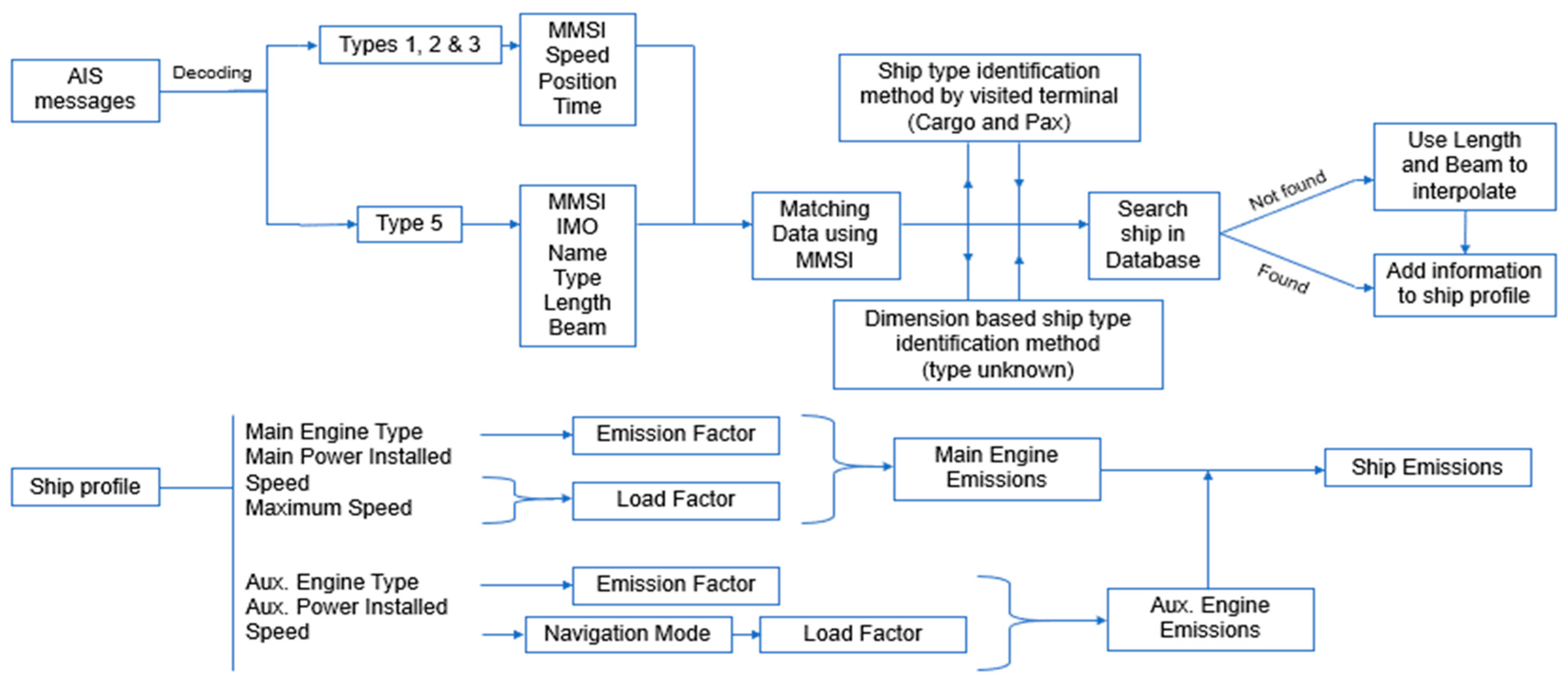The modules of the proposed methodology are illustrated in Figure 1.

Figure 2 provides a more detailed description of the methodology, illustrating for example that AIS data are the main input of this methodology, with the dynamic information of types 1, 2 and 3 messages (ship’s speed, position and time) being matched with static information messages of type 5 (containing the IMO number, the ship’s name, its type, length overall and beam) with correspondent Maritime Mobile Service Identity (MMSI) numbers. This process generates a profile for the ship, describing both its operation and main characteristics. For cases where AIS does not properly identify the type of ship, an alternative method must be used, determining the type of ship based on the visited terminal or the vessel’s dimensions.

This methodology requires technical information of the ships’ machinery, which is not provided by the AIS. For this reason, a database containing main and auxiliary installed powers, engine types (according to its revolution rate, such as slow-, medium- or high-speed diesel engines) and maximum speeds of ships is necessary. If a vessel is identified by the AIS but is not in the database, these technical characteristics are approximated according to the ship’s type, length and beam.

The emission factors used are obtained from the literature [25], and depend on the type of engine as well as the fuel it consumes. As for the load factors for the main engine, these factors are obtained by applying the Propeller Law, using the AIS-provided speed and the maximum ship speed indicated in the database. As regards the auxiliary engines, it will depend on the navigation mode, which itself depends on the ship’s speed. With the emission factors, load factors and installed power the estimated instantaneous emission is obtained.

The proposed methodology is implemented in the numerical tool SEA (Ship Emission Assessment), which divides the process into 5 steps:

(i)

AIS decoding;

(ii)

Area restriction;

(iii)

Ship profile definition;

(iv)

Emission estimation;

(v)

Results preparation.

The first step comprises the decoding of AIS data, from the reading of the files containing AIS messages to the sorting of the necessary information. The second step defines the area of study, identifying ships that navigate through it. Those ships are then associated with their corresponding technical data, producing ship profiles, in the third step. Once the ship’s profile has been defined, instantaneous emission estimates can be calculated in the fourth step. In the fifth and final step, the results of instantaneous emissions are organized to obtain the total amount of emissions and the distributions along the voyage and on a geographical grid. The following sections address with more detail each of these different steps.

3.2. AIS Data Decoding

AIS row messages collected by the Portuguese Coastal Vessel Traffic Service (VTS) Control Centre (CCTMC) are the input for the implementation of the proposed methodology. These messages are decoded with an AIS decoder module that receives raw AIS data files, and decodes the dynamic data (messages of type 1, 2, 3) and the static data (type 5) according to ITU [37]. Then, SEA matches the dynamic and static data using the MMSI number, which is the only common link between them.

3.3. Area Restriction

This step starts with the definition of the study area, which is manually inputted. Then, the implementation tool starts cycling through ships’ positions, eliminating entries whose coordinates are not comprised between the limits established for the latitude and longitude of the study area.

3.4. Ship Profile Definition

Before assigning technical data to each ship, its ship type needs to be properly defined. This is achieved by applying a method developed in this paper and described in Section 4 that defines the type of ship based on the visited terminal. This method’s focus is on ships defined by AIS as “Cargo”, “Passengers” and “HSC”, defining them as “General Cargo”, “Bulk Carrier”, “Container Ship”, “Ferry” and “Cruise”, according to the type of terminal where the ship more often reveals speeds below 1 knot. For ships identified as “Cargo” without speed values below 1 knot, the specific ship type is assigned according to its length overall and beam.

With ship types properly assigned, SEA proceeds to complete ship profiles by adding the correspondent technical data to their already known information. The technical characteristics of interest for emission calculations are the number of main engines, installed power (kW), engine type (diesel, electric, gas turbine), engine speed (slow, medium, high), number of auxiliary engines (generators), power of auxiliary engines (kW). The ship’s service speed and the types of fuel used in the main and auxiliary engines are also important. A ship database that includes these technical characteristics has been developed and used by the proposed methodology. This database is organized by ship type: container ships, tankers, bulk carriers, cruise ships, Ro-Pax and ferries. The information contained in the database is interpolated using the length overall of the ship if the ship is not present in the database or the information is not complete.

When the ship is found in the database, the values of its main engine’s maximum speed, auxiliary engine’s power, type and fuel are assigned based on the parameters contained in the database. The definition of engine type is based on its rated rotations per minute (rpm), with medium-speed diesel engines being assigned values between 300 and 900 rpm. Above this range, the engine is classified as a high-speed diesel engine, and when the rpm is inferior to 300, SEA considers the motor to be a slow-speed diesel engine. It is important that cruise ships are well identified in the database and the value assumed there as the main engine’s installed power (which is going to be used to estimate emissions based on the ship’s propulsion) is shown in [38], 78.2% of the installed power from generators. If the ship is not found in the databases, but its type is well identified, technical characteristics are obtained using the length overall and interpolating data from ships of the same type whose technical information is known.

If the ship, in addition to not being found in the database, has its ship type undefined, default values are assigned to its technical characteristics. These values depend on the length overall (LOA), according to the three different profiles shown in

Table 1. Ship profiles for vessels with unknown technical data.

	Profile 1	Profile 2	Profile 3
LOA (m)	≤20	20 < LOA < 60	≥60
Main Engine Power (kW)	200	1750	$407.25 e^{0.0182LOA}$
Main Engine Type	HSD	MSD	SSD
Main Engine Fuel	MGO	MDO	RO
Auxiliary Engine Power (kW)	0	150	$0.1525P_{ME}+85.064$
Auxiliary Engine Type	-	HSD	MSD
Auxiliary Engine Fuel	-	MGO	MDO
Maximum Speed (knots)	17	13	16

MSD and SSD, respectively, represent high-, medium- and slow-slow-speed diesel engine. MGO—marine gas oil, MDO—marine diesel oil, and RO—residual oil.

. Ships with a length overall smaller than 20 m are assigned to the small ship’s profile (main engine power of 200 kW). From 20 to 60 m, ships are identified with a profile defined based on the technical characteristics of tugs and ferries (main engine power of 1750 kW). Finally, for ships with a length overall larger than 60 m, the profile assigns values of engine power using an exponential regression of general cargo ships in the database, relating the installed power with the length overall. As for the auxiliary engines’ power, a linear regression based on the value of the main installed power is adopted. With the technical characteristics defined, these values are added to the ship trajectory information derived from AIS, producing a complete ship profile for emission assessment.

3.5. Emission Estimation

Methods for ship emission estimations are either defined as top-down or bottom-up. Top-down methods focus on fuel consumption and composition, analyzing the ship’s purchase and supply of fuel, while bottom-up methods focus on ship operation, studying the workloads of the engine in the different modes of navigation and producing more detailed results with the possibility of defining the volume of emissions on a certain geographical area.

This paper develops a bottom-up method that uses AIS data and the ship’s technical characteristics to estimate instantaneous ship emissions at every AIS message timestamp, which are then integrated for the duration of the ship’s operation.

Instantaneous emissions depend on the ship’s main engine and generator characteristics and ship operation and are predicted from information on the installed power, load factors and emission factors of the different power production systems, such as main engines and auxiliary engines, at a given instant, for a given substance.

Having all the data required, SEA cycles through the vector of ship speed values, calculating the emission estimates that vary with the navigation modes and main engine load factor, with both these parameters depending on the ship’s speed. The process of ship emission estimation is described in detail in Section 5.

3.6. Results Preparation

The treatment provided to the values of instantaneous emissions depends on the intent and scope of the study in question. The tool developed provides total values of emissions and geographical distributions for one or more ships, as well as a grid distribution of emissions from port traffic.

Cumulative values of emissions are obtained by trapezoidal numerical integration of ship instantaneous emissions for the duration of this study. As for the geographical distribution of the instantaneous emissions, a color gradient defining the mass of ship emissions along a ship trajectory in the study area is provided. The geographical distribution of ship emissions is derived from the values in the cells of the grid, which are calculated from the accumulated values of instantaneous emissions of ships that cross each grid cell. With the vector of emissions per grid cell, a map of emission levels may be produced, with an image of the area under study in the background.

4. Ship Type Identification Method

A method is proposed to identify the type of ship according to the visited terminal. The approach requires not only the AIS data of the ships (static and dynamic) but also accurate information on the terminals’ locations and types of cargo handled. The location and limits of ports can be easily obtained from geographical information systems and are also clearly defined, in most countries, through national legislation that defines the geographical scope, the concessioned terminal areas and the allowable cargo-handling activities, across the entire port infrastructure. Alternatively, ports and terminal locations can be defined in an unsupervised way by clustering geographic locations of stationary ships (almost zero speed) using, for example, the clustering method OPTICS (Ordering Points To Identify the Clustering Structure algorithm) or DBSCAN (Density-Based Spatial Clustering of Applications with Noise algorithm), as performed by [8].

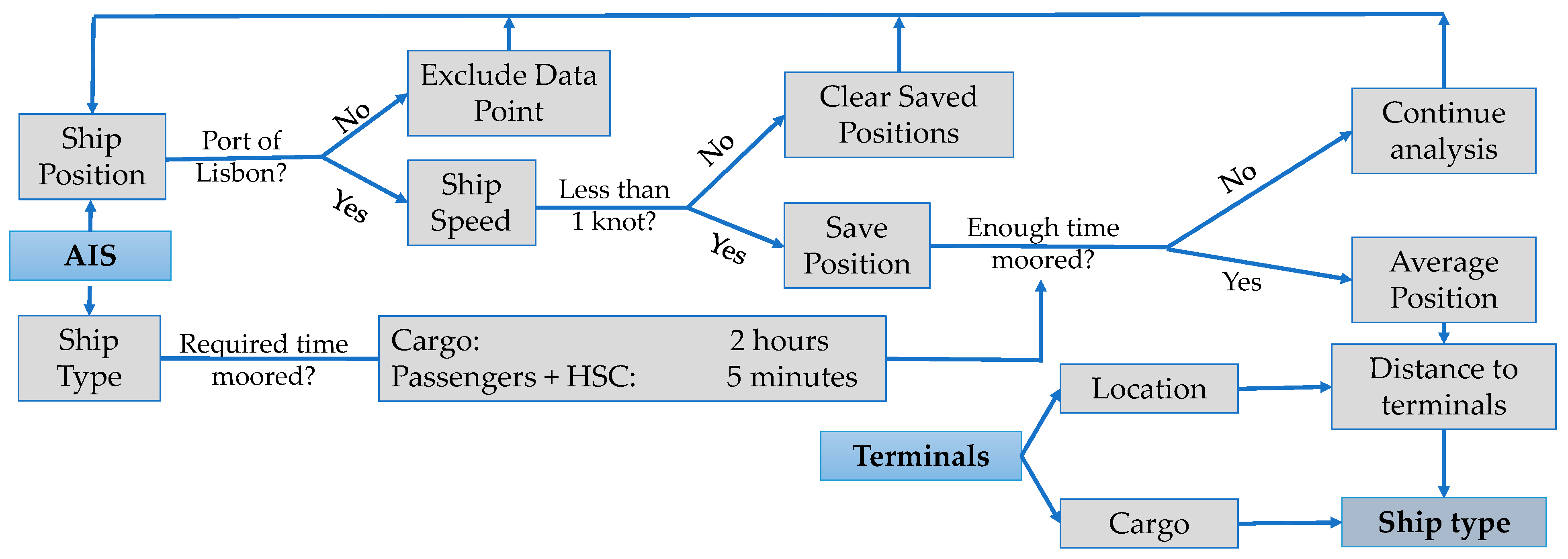
If a comprehensive commercial database is not available, alternative methods, such as this one, can be applied to properly identify the type of ship with a higher level of detail. Figure 3 shows the approach implemented for ship type identification based on the visited terminal. The main inputs of this method are the AIS data, providing broad information on ship type, position and speed, and the terminals’ data.

The method starts by decoding messages of types 1, 2 and 3, saving the operational characteristics of the assigned ship profile when a new MMSI number is detected. This process is repeated for type 5 messages to link the static data with the ship profiles according to MMSI number.

After decoding and matching AIS messages, SEA searches for ships that visited the studied region for a defined duration. This selection is performed by comparing ship positions against the limits of the area of study. A second selection is made to exclusively obtain ships whose AIS-defined types matched those targeted by this method (“Passenger”, “Cargo” and “HSC”).

To determine which terminal is visited by a particular ship, SEA registers ship positions with speeds slower than 1 knot, defining its navigation mode as moored. One very important aspect is the elimination of the saved mooring positions until the speed rises above 1 knot. This reduces the chances of manoeuvring ships registering mooring positions away from the visited terminal.

For ships characterised as “Cargo” by AIS, the method assumes that the ship is visiting a terminal when it is moored for more than 2 h. The mooring position detected is averaged with the previous four positions received from AIS. As for “Passenger” and “HSC”, the time interval is reduced to 5 min, due to the short mooring time of ferries, and the registered position is averaged with only the latest 2 points.

After establishing the average position while berthed, SEA calculates the distance to each terminal, using the orthodromic distance. By comparing the distance to each terminal, the shorter value produces an assumption of ship type. This process is repeated for every call detected for the duration of this study, defining the ship type as the one most frequently assumed for the ship.

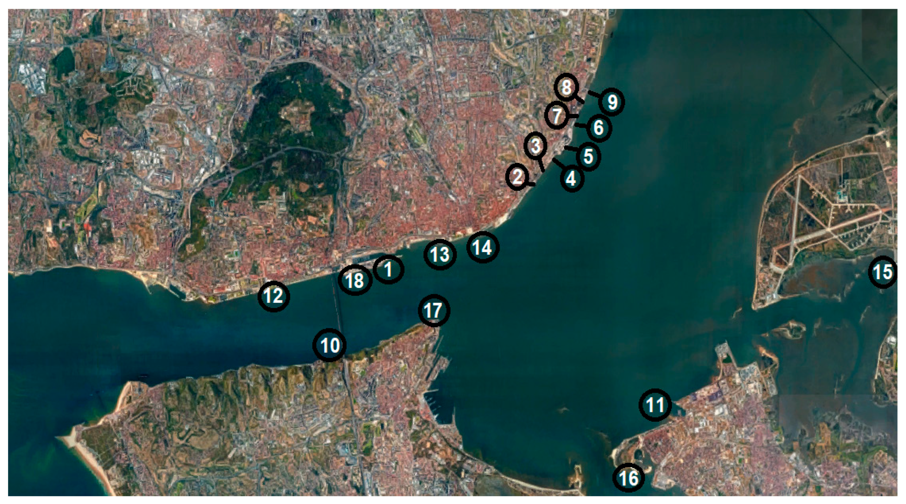
The efficiency of this process was evaluated by analyzing the ships that called the port of Lisbon in a given period. Detailed information on the ship types is obtained from Marine Traffic’s website. Figure 4 illustrates the location of the studied terminals within the port of Lisbon.

Table 2. Success rate of the ship type identification method.

Ship type	Number of Ships	Ship Types Correctly Identified	Success Rate of Ship Type Identification Method
Ferry	27	27	100%
Cruise	17	16	94.1%
Bulk carriers	10	7	70%
Container	69	58	84.1%
General cargo	58	41	70.7%
Fishing	1	0	0
Other passenger ships	44	43	97.7%
Cargo	139	107	77%
Total	183	149	81.4%

shows the absolute number of ships detected between 9 July and 9 August 2008, and the corresponding success rates of the ship type identification method.

The application of the ship type identification method to the marine traffic at the port of Lisbon in the study period correctly identified 100% of the ferries and 97.7% of the passenger ships, with a single ship being misidentified in these categories. For cargo ships, however, the success rate tends to decrease, with bulk carriers and general cargo ships registering values between 70% and 84%. This is mainly due to the existence of multipurpose terminals and ships that visit terminals of different types. The global success rate of the identification of ship types based on the visited terminal is 81.4%, which is an acceptable value allowing, at least for port traffic, its inclusion into the ship emission estimation methodology proposed in this paper.

5. Estimation of Ship Emissions

The calculation of instantaneous emissions in grams per second (e) is carried out using:

$$e=\frac{P\times LF\times EF}{3600}$$

(1)

According to Equation (1), the instantaneous emissions are estimated by the product of the power (P), load factor (LF) and emission factor (EF). The denominator converts the output units from grams per hour to grams per second, since, for convenience, the power is given in kilowatts, the load factor is adimensional and the emission factor (EF) shall be in grams per kilowatt-hour.

A ship’s instantaneous emission corresponds to the summation of the results of Equation (1) applied to the different power production systems, such as main engines and auxiliary engines, at a given instant and mode of navigation, for a given type of fuel.

The main source of the ship’s gaseous emissions is the exhaust combustion products from the power production systems, resulting in a direct relationship between the mass of emissions and the installed power onboard. It is difficult to estimate the installed power based on the data provided in the AIS messages, especially the installed power of generators and boilers. For this reason, this information is derived from the application of the approach described previously in Section 3.4 using a database of ships’ technical characteristics and specific ship profiles for vessels with unknown technical data.

5.1. Modes of Navigation

Typically, there are three main modes of ship navigation: berthed (loading or unloading), manoeuvring (usually when entering or leaving the port) and cruising (travelling between ports). These three modes of navigation are defined based on the ship’s speed, as performed in [39,40]. Similarly to [41], the limits assumed determine that cruising ships move at speeds higher than 5 knots while manoeuvring ships circulate with speeds between 1 and 5 knots and berthed ships are allowed a margin of 1 knot (instead of a stand-still situation of zero knots), due to the AIS precision.

Figure 5 shows the different navigation modes according to the ship’s speed coming from the AIS data. Entering the port in the cruising mode, there’s a speed reduction indicating probably a waiting period for the pilot vessel. Closer to the terminal, there is another speed reduction, this time probably associated with the manoeuvring and mooring of the ship.

5.2. Load Factors

Engines are designed to work with a certain load, but during their operation, it is impossible to maintain the same loading condition. These differences in the workload of the engine affect the fuel consumption of the ship and consequently its emissions. As in [26], it is assumed that the power provided by the ship’s main engine is fully allocated to its propulsion, while the generators provide power to the other ship systems, the exception being cruise ships with diesel–electric propulsion, with 78.2% of generators installed power supplying the propulsion system (when cruising), as in [38].

5.2.1. Main Engine Load Factor

The main engine workload is directly related to the ship’s speed, and, as the Propeller Law states, “the necessary power delivered to the propeller is proportional to the rate of revolution to the power of three” [42]. However, extrapolating this proportionality to the relation between the engine-installed power and the ship speed requires some assumptions:

• The efficiency of the power production system and the shaft line are constant for different engine loading conditions, with the installed power being proportional to the power of the propeller.
• The propeller’s pitch is fixed, ensuring the proportionality of the ship’s velocity and the propeller’s rotating speed. This assumption is necessary since, with controllable pitch propellers, the same values of maximum ship speed and the propeller’s maximum and instantaneous rates of revolution, may generate different values of instantaneous ship speed.

This way, the load factor can be calculated as the ratio between the power of three instantaneous (i) and maximum (max) vessel speeds:

$$LF=\frac{P_{{ME}_{instant}}}{P_{{ME}_{installed}}}=\frac{C_1\times P_{{prop}_i}}{C_1\times P_{{prop}_{max}}}=\frac{C_2\times {n_{{prop}_i}}^3}{C_2\times {n_{{prop}_{max}}}^3}=\frac{C_3\times {V_{{ship}_i}}^3}{C_3\times {V_{{ship}_{max}}}^3}=\frac{{Instantaneous Speed}^3}{{Maximum Speed}^3}$$

(2)

where C₁, C₂ and C₃ are constants. The obtained load factor is applied to the main engine’s installed power.

5.2.2. Auxiliary Engines Load Factors

In different modes of navigation, auxiliary engines have different workloads, with the maximum values usually occurring at the beginning and end of a voyage or during loading/unloading operations, being independent of ship speed. Due to the endless variables influencing the instantaneous workload of the generators, this paper considers fixed values for the auxiliary engines’ load factor depending on the ship type and navigation mode, as suggested by [25] and shown in

Table 3. Auxiliary engines’ load factors according with [25].

	Auxiliary Engines’ Load Factors (%)
At sea	30
In port (tankers)	60
In port	40
Maneuvering	50

. Load factors are considered to be similar for every type of ship, except for tankers, due to the additional power supplied to pumps during loading/unloading operations.

Applying the same load factors for every ship type may be considered a rough assumption. However, most cargo ships operate in similar circumstances, except passenger ships, which typically register higher load factors due to the necessity of supplying large accommodations and public spaces. However, for the case of ferries the installed power of auxiliary engines is usually low (for ferries in the port of Lisbon auxiliary engines represent between 1.8% and 2.6% of the total installed power) and the case of cruise ships with diesel–electric systems is a particular one, with load factors according to [38] and depending on the season (summer or rest of the year), as shown in

Table 4. Auxiliary engines’ load factors for diesel–electric cruise ships according with [38].

	Auxiliary Engines’ Load Factors—Cruise Ships (%)
	Summer	Rest of the Year
At sea	30	30
At berth	60	40
Maneuvering	75	60

. This distinction between seasons is justified by the increased demand for air conditioning during summer, as it is of utmost importance for cruise ships to guarantee their passengers’ comfort while having a significant impact on emissions in port, as shown in [24].

5.3. Emission Factors

In addition to the ship’s performance or power production systems, many other factors influence the mass of exhaust gases, while some are easier to measure than others. Entec [25] developed emission factors to quantify ship emissions without the need to apply corrective coefficients to adjust the results for each of the infinite aspects that may affect the estimations produced by ships. These factors were derived by combining emission databases, from the IVL Swedish Environmental Research Institute and the Lloyds Register Engineering Services, with the European Commission’s database of ships circulating in the North Sea, Irish Sea, English Channel, Baltic Sea, Black Sea and the Mediterranean. Entec [25] has analyzed 608,942 ship movements, in the designated area, during four months of study in the year 2000, presenting tables of the derived emission factors for the substances NO_x, SO_x, CO₂, HC and PM, depending on the type of engine installed (slow, medium or high speed) as well as the type of fuel being consumed (marine gas oil, marine diesel oil and residual oil) and the navigation mode (at sea, manoeuvring and in port). Since then new sets of emission factors have been developed based on statistical analyses of ships’ emissions available in literature obtained from a multitude of techniques, as reviewed by [43].

Table 5. Main engine emission factors for the cruising mode (values in g/kWh) according with [25].

	NOX	SO2	CO2	HC	PM
SSD/MGO	17.0	0.9	588	0.6	0.3
SSD/MDO	17.0	3.7	588	0.6	0.3
SSD/RO	18.1	10.5	620	0.6	0.8
MSD/MGO	13.2	1.0	645	0.5	0.3
MSD/MDO	13.2	4.1	645	0.5	0.3
MSD/RO	14	11.5	677	0.5	0.8

SSD and MSD, respectively, represent slow- and medium-speed diesel engines. MGO stands for marine gas oil, while MDO and RO stand for marine diesel oil and Residual Oil, respectively.

shows the emission factors taken from a segment of the above-mentioned tables for slow- and medium-speed diesel engines. By observation of Table 5, it is noticeable that while SO₂ emission factors depend considerably on the type of fuel, NO_X emission factors depend on the type of machinery installed. CO₂ follows the pattern of SO₂ but on a less evident degree and much larger scale (larger specific values).

5.4. Low Load Adjustment

Even though the relation between the engine’s workload and its emissions is, in general, directly proportional, there is a situation, usually associated with manoeuvring ships, when the mass of the emissions increases with the decreasing load factor.

Regression equations of emission rate as a function of fractional load are used to obtain proper emission estimates for ships working with low main engine loads (load factor at 20% or lower), as in [28]. These regressions were developed with data from the results of emission tests performed on a sample of 291 ships by [28]. While the remaining exhaust gases are directly associated with the main engine’s load factor, USEPA’s report portrays SO₂ emission rate as a function of the sulfur flow (defined by the emission factor).

Equations (3) and (4) illustrate the regression lines’ equations, while

Table 6. Coefficients a, b and x for the different emission substances and corresponding regression coefficient of determination.

	NOX	SO2	CO2	HC	PM
a	0.1255	2.3735	44.1	0.0667	0.0059
b	10.4496	−0.4792	648.6	0.3859	0.2551
x	1.5	-	1	1.5	1.5
r2	0.57	0.78	0.65	0.52	0.95

presents the coefficients a, b and x, as well as the coefficient of determination (r²). The low load adjustment factor is, for NO_x, CO₂, HC and PM:

$${LL}_{adj} \left\{{\mathrm{N}\mathrm{O}}_{\mathrm{x}},{\mathrm{C}\mathrm{O}}_2,\mathrm{H}\mathrm{C},\mathrm{P}\mathrm{M}\right\}=a {\left(FL\right)}^{-x}+b [\mathrm{g}/\mathrm{k}\mathrm{W}\mathrm{h}]$$

(3)

where FL represents the fractional load. For SO₂, the low load adjustment factor is:

$${LL}_{adj} \left\{{\mathrm{S}\mathrm{O}}_2\right\}=a \left(EF\right)+b [\mathrm{g}/\mathrm{k}\mathrm{W}\mathrm{h}]$$

(4)

where EF represents the emission factor.

Analyzing Equation (3) and Table 6, it is possible to see that the coefficient b represents the base value for the new emission factor, coefficient x defines the inverse relation with the load factor (the emission factor rises with the decreasing of the load factor) and coefficient a describes the rate of proportionality.

As for Equation (4), applicable to the particular case of SO₂ emissions, the negative value of b might indicate that SO₂ emissions could possibly be lower under low-load operation. However, this only occurs if the original emission factor is smaller than 0.349 g/kWh. As the smallest load factor of those applied in this paper is 0.9 g/kWh (see Table 6), the inverse proportionality between load factor and emission factor for SO₂ emission during low load operation is confirmed. It should be noted the higher value of the coefficient of determination of SO₂’s regression, than the equivalent expressions for NO_X and CO₂. This higher value supports the assumption that SO₂ emissions depend more on the type of fuel (weighted on the emission factor determination) than the engine’s load factor.

6. Case Studies

The methodology proposed in the previous sections is now applied to three different case studies. The first one refers to the maritime traffic of passenger ships in the port of Lisbon, comparing emissions of a ferry connecting the north and south banks of the Tagus River (Cais do Sodré to Barreiro) with a cruise ship calling at the port of Lisbon’s Alcântara terminal. The motivation for this study stems from the substantial traffic of river ferries used as public transportation on a daily basis, and the also substantial traffic of cruise ships visiting Lisbon. The accuracy of the proposed methodology is assessed by applying another methodology [22] to the data of this study and by applying the methodology proposed in this paper to data from a third study [23]. The second case study addresses ship emissions of vessels navigating in the port of Lisbon, presenting its results through a geographical distribution of emissions, as this distribution may have a substantial impact on the north bank of the river where the city itself is located and this has been criticized by environmentalists. The third and final case study demonstrates the application of this methodology also to coastal maritime traffic, showing the emissions of a single ship throughout its voyage along the Portuguese western coast. The motivation for this particular case is the fact that this coastline is one of the busiest tradelanes in Europe with hundreds of ships moving north and south every day.

6.1. Cruise vs. Ferry Emissions at the Port of Lisbon

This case study addresses the emissions of a cruise ship, from the moment it enters the port to the moment it leaves (8.7 h), against the ones from a smaller but more active ferry, for the same period, comparing the results obtained with the presented methodology when applied to two known vessels.

Table 7. Ship’s technical characteristics.

	Cruise Ship	Ferry
Propulsion	Electric	Mechanic
Propulsion Power (kW)	28,000	4640
Main Engine Type	-	HSD
Main Engine Fuel	-	MGO
Total Generator Power (kW)	46,080	168
Generator Type	MSD	HSD
Generator Fuel	MDO	MGO
Maximum Speed (knots)	22.4	30

describes their technical characteristics, with MSD standing for medium-speed diesel; HSD for high-speed diesel; MDO for marine diesel oil; MGO for marine gas oil, while

Table 8. Ship’s time distribution per navigation mode (in minutes).

	Cruise Ship	Ferry
Moored	437	218
Maneuvering	17	25
Cruising	69	281
Total	523	523

shows the time spent in each navigation mode.

Despite both ship types being dedicated to the transport of passengers, there is a significant difference in the operations of a cruise ship and a ferry, inside a port, with the ferry being more active and spending most of the time navigating its everyday route while the cruise ship is moored for most of the call’s duration. Regardless of its more active operation than the cruise ship, as Table 8 illustrates (with a difference of 220 min in time spent navigating), with emissions nearly 3-fold higher than the moored Cruise ship, the Ferry spent 42% of the duration of this study moored, emitting almost 350-fold less than the Cruise ship in the same navigation mode. This was identified as a major cause for the discrepancy observed in the results of total emission estimations.

The cruise ship emissions are estimated as 936 kg, 297 kg, 47.978 tons, 0.033 tons and 0.021 tons of NO_X, SO₂, CO₂, HC and PM, respectively, as shown in

Table 9. Cumulative emission estimates for a cruise ship and a ferry.

	Cruise	Ferry	Cruise/Ferry
NOX (t)	0.936	0.054	17.33
SO2 (t)	0.297	0.020	14.85
CO2 (t)	47.978	3.042	15.77
HC (t)	0.033	0.0019	17.37
PM (t)	0.021	0.0014	15

. For the Ferry, emissions are estimated as 54 kg, 20 kg, 3042 kg, 1.9 kg and 1.4 kg of NO_X, SO₂, CO₂, HC and PM, respectively, representing a mass of emissions 14.85- to 17.37-fold lower than those of the cruise ship. The accuracy of these first results of emission estimates was tested against the methodologies of [22,23], revealing relative differences in the results lower than 15%.

In terms of instantaneous emissions of NO_X, the maximum registered value for the ferry in the cruising mode is 67.5 g per second, while for a moored cruise ship, this value is 28 g per second. However, when moored, the ferry emits only 0.2 g of NO_X per second, which is approximately 140-fold less than the moored cruise ship. As the ferry is moored for 42% of the study duration, the NO_X total emissions of the cruise ship are still higher (17.33-fold higher, as shown in Table 9).

6.2. Distribution of Emissions in the Port of Lisbon

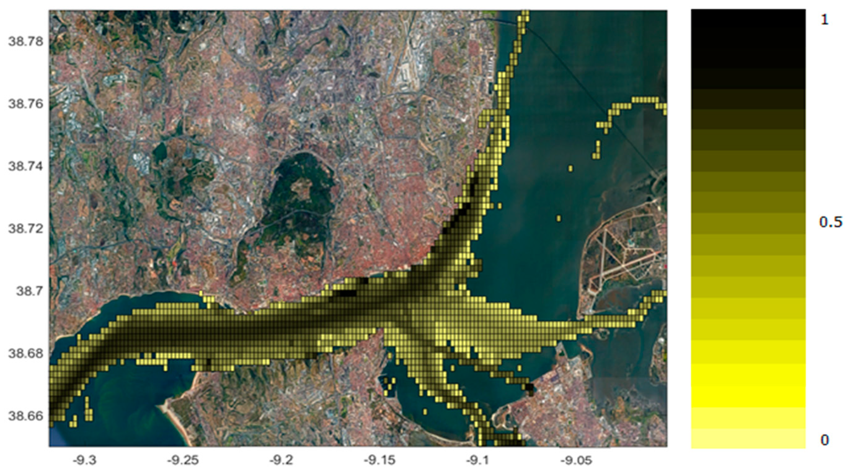
The port of Lisbon spreads through the mouth of Tagus River, along both of its banks. It is of the utmost interest to assess the distribution of ship emissions throughout the port of Lisbon’s geographical domain, providing information on the most affected regions, as the port is located very close to densely populated areas. This was carried out by the tool SEA, presenting a grid distribution, with each cell representing an area of 222 by 174 m, estimating emissions of port traffic from 9 July to 9 August 2008. Before proceeding with the estimation of emissions, the fleet under study was divided per ship type, averaging each type’s technical characteristics, as shown in

Table 10. Fraction of the observed fleet and averaged technical characteristics per ship type.

	Fleet (%)	ME Power (kW)	AE Power (kW)	Length (m)	Beam (m)
Ferry	30.79	2423	60.7	41.77	10.37
Cruise	1.14	22,831	23,492	226	28.83
Tanker	7.70	4567	1404	125.15	19.3
Bulk	7.39	6863	1214	160.94	22.7
General Cargo	16.58	3504	619	105	17.89
Container	17.46	10,843	2389	152.97	26.9
Port Ops	11.36	526	0	14.54	4.79

. An example of the resulting distribution is shown in Figure 6, in this case regarding the emissions of CO₂. Due to the large difference in the order of magnitude from emissions with heavy and scarce emissions, the results were plotted as the logarithmic scale of the ratio to the maximum registered value (highest concentration of instantaneous emissions per cell registering 115 g, 55 g, 5645 g, 4.8 g, 4.1 g of NO_X, SO₂, CO₂, HC and PM, respectively).

Figure 6 shows that the higher values of emissions appear in coastal areas where the terminals are located (namely along the north bank of the river, where the most densely populated areas are located). There are also a couple of high-emission areas located along the navigation channels to the south bank (ferry connections). To better evaluate the distribution of emissions, these were divided per ship type, and the results are shown in

Table 11. Total emissions per ship type.

	NOX (t)	SO2 (t)	CO2 (t)	HC (t)	PM (t)
Ferry	58.70	6.80	3180.1	1.40	1.50
Cruise	22.40	7.10	1123.9	0.70	0.50
Tanker	4.10	1.40	231.9	0.15	0.13
Bulk	16.67	4.86	964.3	0.61	0.53
General Cargo	5.65	1.87	283.2	0.18	0.14
Container	37.90	13.50	2006.1	1.40	1.10
Port Ops	1.29	0.11	67.7	0.06	0.03
Others	1.41	0.12	74.4	0.06	0.04
Total	148.1	35.8	7931.6	4.6	4.0

. Regarding total emissions, the exhaust product with higher values was carbon dioxide, with 7999 tons, 53.5-fold higher than the emitted mass of nitrogen oxides, the second higher, with 149.4 tons. The emissions of sulfur dioxide reached 36.9 tons. While container ships were the main contributors to SO₂ emissions, ferries emitted more of the remaining exhaust products.

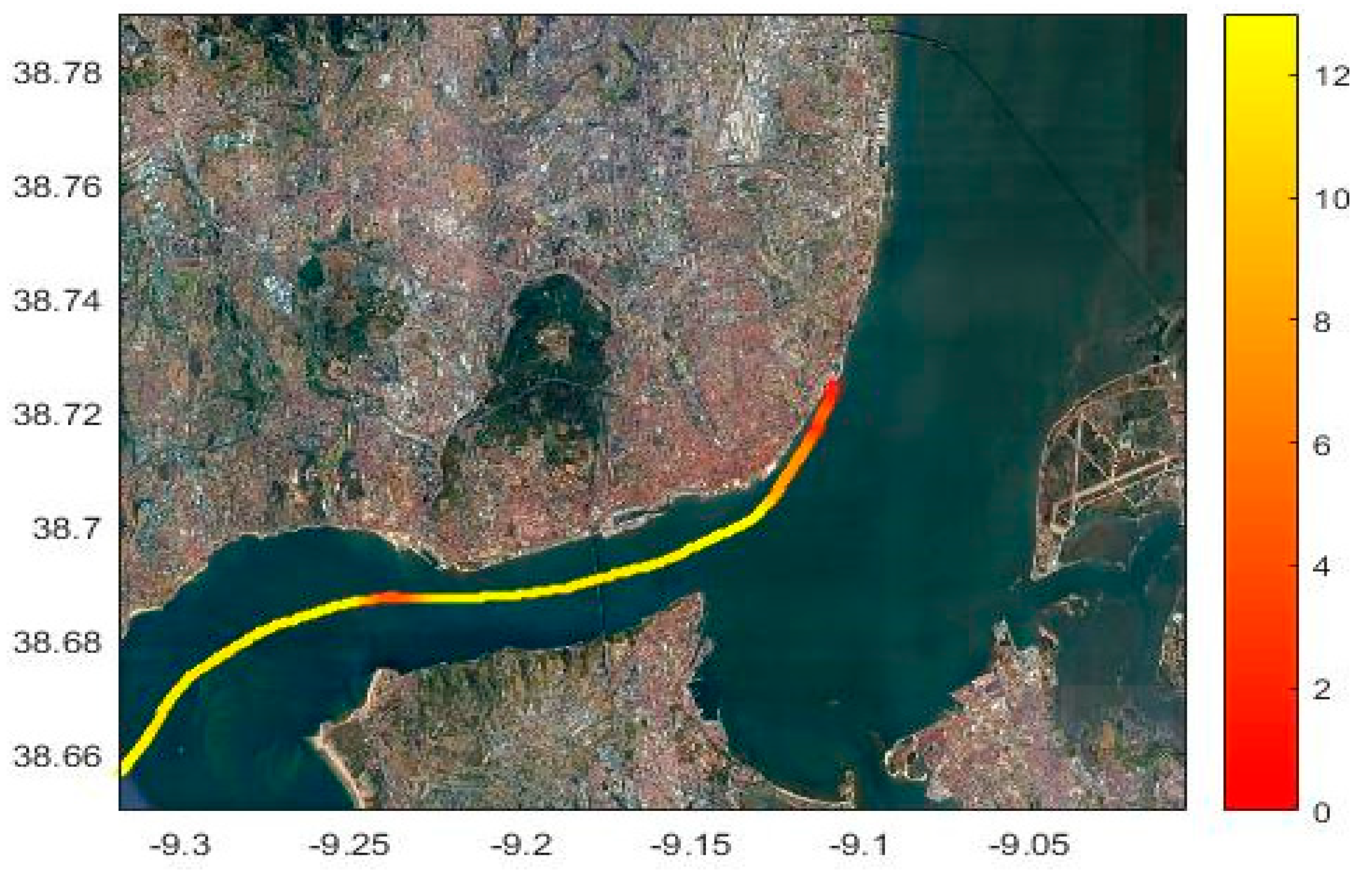
6.3. Ship Cruising along the Portuguese Coast

This case study addresses the emissions of a container ship, whose technical characteristics are known (shown in

Table 12. Container ship technical characteristics.

	Container Ship
LOA (m)	261
Beam (m)	32.3
Main Engine Power (kW)	24,300
Main Engine Type	SSD
Main Engine Fuel	RO
Total Generator Power (kW)	3990
Generator Type	MSD
Generator Fuel	MDO
Maximum Speed (knots)	22

). In this table, SSD stands for slow-speed diesel; RO stands for residual oil; MSD stands for medium-speed diesel; MDO stands for marine diesel oil). The ship is navigating along the Portuguese coast, first heading north and then heading south 8 days later, not calling at any Portuguese port for the duration of this study, but representing the case of hundreds of ships that sail daily along the Portuguese coast.

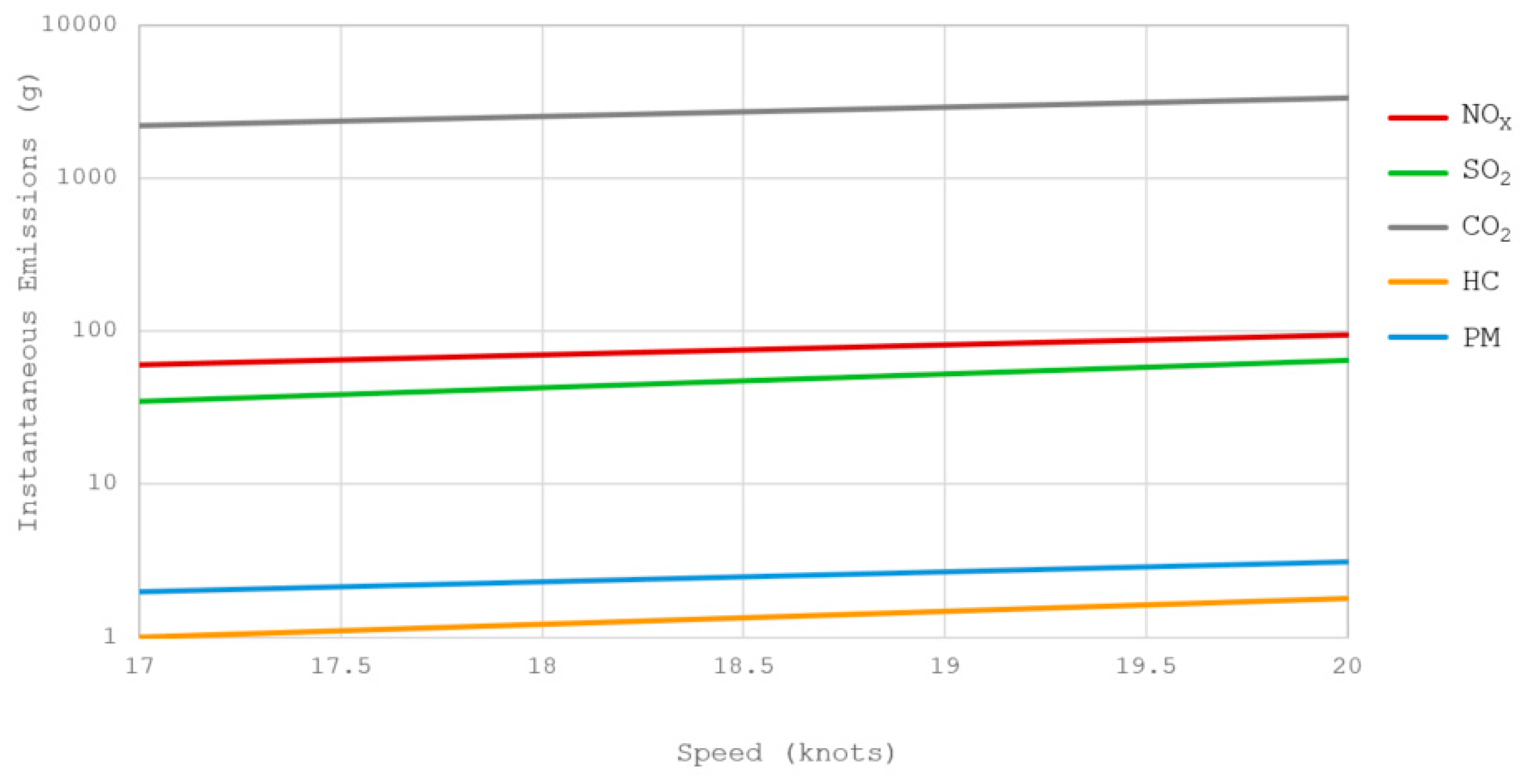
The vessel is first detected by AIS during its route heading north. In this leg of the voyage, its journey along the Portuguese coast lasted 17.6 h, registering an average speed of 18.3 knots, which would represent a distance travelled of 322 nm. Eight days after the first time it was detected, the container ship initiated a second crossing of the Portuguese coast, this time heading south, for 19.1 h, averaging 18.5 knots through a 354 nm course.

For a single ship operating in the cruising mode, the auxiliary engine’s operation remains constant and both the main engine’s installed power and emission factors also remain unaltered, with the only changed parameter being the main engine’s load factor, depending on the cube of the ship’s speed; therefore, there is a direct proportionality between the value of instantaneous emissions and the cube of the ship’s speed. Figure 7 presents a graphical display of this relation.

For the first voyage, SEA estimated 4.767 tons, 2.686 tons, 167.8 tons, 0.157 tons and 0.204 tons of NO_X, SO₂, CO₂, HC and PM, respectively. The second voyage registered more emissions, as it was expected due to its higher average speed, duration and bigger length. The values obtained were 5.325 tons, 3.003 tons, 187.3 tons, 0.175 tons and 0.228 tons of NO_X, SO₂, CO₂, HC and PM, respectively.

7. Conclusions

This paper proposes and develops a methodology to estimate ship emissions based on data available in messages of the Automatic Identification System. A computational tool is created that implements the proposed methodology and includes an alternative method designed to identify ship types based on the visited terminal. This ship type identification method, when applied to the port of Lisbon’s traffic, correctly identified 100% of the ferries, 97.7% of the passenger ships and between 70% and 84% of the cargo ships, resulting in a global success rate of 81.4%. Most incorrect identifications were due to the existence of terminals that actually receive several ship types in the area under study.

As regards the emissions estimates, despite the ferry having a more active operation than a cruise ship, the latter registers a much higher mass of emissions. In fact, the ferry spends 42% of the duration of this study moored, emitting approximately 140-fold less than the cruise ship in this navigation mode. This is identified as a major cause of the higher total emissions estimated for the cruise ship compared to those of the ferry (between 15- and 17-fold higher). Furthermore, ferries represent approximately 31% of ship calls at the port of Lisbon, followed by container ships and general cargo ships, with respective representations of 17.5% and 16.6%.

It was concluded that the low value of SO₂ emissions was a consequence of the predominance of ferries over the global emissions, since most of these vessels are equipped with high-speed diesel engines fuelled with marine gas oil that has sulfur content of 0.1%. Additionally, it is also associated with the enforcement from the port of Lisbon of the Community Directive 2005/33/EC that regulates the sulfur content of the fuelled used by ships as well as the fuel supplied by oil companies, prohibiting fuels with sulfur concentrations above 1.5%. When operating in the cruising mode, without reducing the main engine’s load below 20%, emission estimates depend only on the ship’s speed, with a linear relationship between the instantaneous emissions and the cube of the instantaneous ship speed.

As a final conclusion, the performance of the alternative method of ship type identification based on the visited terminal and the comparison of the ship emission estimates with the ones obtained from other two methodologies indicate that the methodology developed is not only accurate but also independent of commercial databases, which was one of the objectives of this paper. The numerical results support the current policy of the Port Authority of Lisbon of introducing shore power supply for cruise ships calling in Lisbon and the option of the public transport company Transtejo of investing in electric river ferries.

As recommendations for further work, the methodology proposed in this paper can be improved by establishing up-to-date empirical and probabilistic models to determine the technical characteristics of ships, allowing its immediate application to world maritime traffic. As a suggestion for future studies, AIS could be used to evaluate port queues and its environmental impacts, due to the unnecessary time in port spent by ships, observable in their trajectories described by AIS positions. Another interesting topic to be developed would be the assessment of water contamination from port traffic, associated with the utilization of humid exhaustion of main engines, as used nowadays in some ferries and towing vessels.

Regarding ship emissions, the AIS has the potential to be used in the future to assess and control emissions of the world fleet, in real-time. As there are messages in AIS dedicated to dynamic and static data, a new type of message could be included, reporting environmental data and values of instantaneous emissions, power consumptions and type of fuel being used.