The Two-Parameter Holland Pressure Model for Tropical Cyclones

Abstract

In this study, we propose a two-parameter symmetric tropical cyclone (TC) pressure model, derived from the fundamental equations of the TC wind field. This model rectifies the deficits of the traditional TC pressure model mathematically. It incorporates a new parameter into the Holland pressure model and establishes relationship equations between the new parameter, Holland parameter B, and TC attributes such as pressure difference, maximum wind speed radius, geographical latitude, and inflow angle. This derivation is achieved theoretically. Our model not only tackles the limitations of the traditional pressure model by meeting the gradient wind equations, but it also resolves the uncertainty issue of parameter B arising from varied factor selection, data time frames, and research maritime areas. As practical applications, we apply both this model and the corresponding wind field model to five TC profiles. Further, we juxtapose them with primary pressure and wind field models and conduct error and statistical significance analyses. Our findings reveal that the two-parameter model produces results on par with the Holland model and superior to Fujita and Takahashi models. Notably, reanalysis of the wind field consistently underestimates the wind field near the maximum wind speed. Hence, a hybrid wind field, synthesized from the modeled and reanalyzed wind fields, appears to be one of the most effective methodologies for reconstructing a tropical cyclone’s wind field.

1. Introduction

Tropical cyclones, a category of intense storms originating in tropical oceans, primarily impact three major sea regions globally: the Northwestern Pacific Ocean, the North Atlantic Ocean, and the Indian Ocean. As these storms approach or hit continents, they cause severe natural disasters, including powerful winds, heavy rainfall, storm surges, and mudslides, among others. According to Southern (1979), the annual global economic loss due to tropical cyclones in the 1970s amounted to USD 6–7 billion, with a fatality count of 20,000, ranking the phenomenon amongst the top ten natural disasters [1]. In his study, Emanuel (2005) analyzed global tropical cyclone data, concluding that these storms’ risk increased between 1975–2004 due to global climate change effects. He also predicted further intensification of these hazards in coastal areas as populations continue to increase [2]. Muis (2016), utilizing global storm surge and extreme sea level reanalysis data, projected that 1.3% of the global population would be vulnerable to 100-year flooding resulting from tropical cyclones [3]. Tiwari (2021) analyzed satellite data from 1979–2018 to study post-monsoon tropical cyclone variability trends over the Bay of Bengal. He used the Accumulated Cyclone Energy (ACE) and Power Dissipation Index (PDI) as metrics [4].

Tropical cyclone wind fields primarily result from pressure gradient forces, necessitating the creation of predictive models for both pressure and wind fields of these cyclones. Such models aid in assessing the damage tropical cyclones can cause to infrastructure, production, and the lives and properties of coastal inhabitants. Broadly, these pressure and wind field models can either be parametric or numerical. Numerical models like WRF and MM5 are often employed in specialized fields like catastrophic science due to their complexity. However, their demand for significant computational resources and long simulation times often compromises their timeliness. Conversely, the simplicity and guaranteed computational accuracy of parametric models make them a popular choice. This paper focuses on symmetric pressure and wind parametric models, though recent research has also explored asymmetric parametric models [5].

In the polar coordinate system, the gradient wind equation for a tropical cyclone is defined as follows:

$$\frac{V^2}{r}+fV=\frac{1}{{\rho }_a}\frac{\partial \mathrm{P}}{\partial r}$$

(1)

In this equation, $V$ and $P$ represent wind speeds and pressures at $r$ distance from the center of a tropical cyclone, respectively. $f$ is defined as the coefficient of Coriolis force, represented as $f=2\Omega \sin \phi$. Here, $\Omega$ symbolizes the angular velocity of the earth’s rotation, while $\phi$ i stands for the geographical latitudes. Additionally, ${\rho }_a$ is the air density.

The parameterization of a tropical cyclone’s wind field model is heavily dependent on the air pressure field model. Over nearly a century of exploration, numerous scholars have advanced a significant number of air pressure models that hold paramount research significance and practical value.

Observations from the weather station reveal that the pressure curve exhibits characteristics of a funnel-shaped section. Therefore, the pressure of a tropical cyclone can be approximated by a symmetrically distributed set of concentric circles. Based on this understanding, Vilhelm Bjerknes in 1921 established the following pressure model [6]:

$$P=P_n-\frac{\mathsf{\Delta }P}{1+(r/R{)}^2}$$

(2)

In Equation (2), $R$ represents the radius of the maximum wind speed. Differential pressure, identified as $\mathsf{\Delta }P$, is identified as $P_n-P_c$ where $P_n$ is the ambient pressure and $P_c$ is the central pressure.

As observational data increased, Takahashi [7] revised the empirical model originally developed by Horiguti [8] in 1926. This revision, proposed in 1939, was based on data from the Japan Meteorological Agency weather map and involved the establishment of the following pressure model:

$$P=P_n-\frac{\mathsf{\Delta }P}{1+r/R}$$

(3)

Tropical cyclones are generally categorized into two regions: internal and external. The internal region encompasses the area near the cyclone’s center, characterized by a parabolic pressure profile. Conversely, the external region has a hyperbolic pressure profile. Importantly, in the referenced model, Formula (2) renders a more accurate simulation of the pressure for the internal region than the external one. In contrast, Formula (3) better simulates the external air pressure over the internal air pressure. Subsequently, in 1952, Fujita proposed the following model [9]:

$$P=P_n-\frac{\mathsf{\Delta }P}{{\left[1+2{\left(r/R\right)}^2\right]}^{1/2}}$$

(4)

Upon computation and analysis of accumulated observational data, it has been determined that the simulation efficiency of Fujita’s model is occasionally inferior to that of the Takahashi model in the external field of a tropical cyclone. Consequently, some scholars [10] proposed a sectional structure model implementing Fujita’s method for the internal field and Takahashi’s method for the external field.

In 1954, Schloemer [11] introduced an exponential pressure model, distinguishing itself from the prior three pressure models.

$$P=P_c+\mathsf{\Delta }P{e}^{-R/r}$$

(5)

While the aforementioned four pressure models can simulate the atmospheric pressure profile characteristics of tropical cyclones to a certain degree, their simplicity in structure prohibits them from possessing the necessary parameters to modulate the physical process of atmospheric pressure and profile structural characteristics. This results in their inability to fully reflect the variability among different tropical cyclones. This led Holland to analyze the measured pressure profiles of nine tropical cyclones in Florida in 1980 [12]. The analysis revealed differences in the rates of radial variation of the pressure differential across different tropical cyclones. Building upon Schloemer’s exponential pressure model [11], Holland introduced a pressure profile parameter B, thereby establishing the following parametric pressure model:

$$P=P_c+\mathsf{\Delta }P{e}^{-{\left(R/r\right)}^B}$$

(6)

The Holland model, known for its ability to accurately depict the atmospheric pressure profile of a tropical cyclone, is widely utilized. The core of simulating the atmospheric pressure and wind field of a tropical cyclone lies in the selection of the atmospheric pressure profile’s B parameter. Over four decades, numerous scholars have conducted extensive research on the relationship between the B parameter and influencing factors. Vickery [13,14], Willoughby [15], and Holland [16] each proposed formulas relating the B parameter to the structure and physical characteristics of tropical cyclones. The factors involved mainly include pressure differences, maximum wind speed and its radius, and geographical latitude. Holland [16] proposed the most complex formula, involving six influencing factors. Fang [17], by investigating key parameters including the radius of maximum wind and the Holland B, constructed a parametric wind field model suitable for typhoons in the western North Pacific Ocean. Hu et al. [18] used the Holland pressure model and degree wind equation to account for Coriolis effects in parameter B, resulting in a 20% accuracy increase for large but weak tropical cyclones. Sun [19] employed a backpropagation neural network to estimate the Holland B parameter. Zhong [20] developed a framework that contemplates the azimuth-dependent Holland B parameter. Despite the empirical nature of these formulas, resulting from a statistical analysis of observed data, they lack a solid theoretical foundation. They exhibit strong collinearity problems amongst some influencing factors, such as the wind–pressure relationship. Some formulas are easy to use but lack precision, while others, despite their high accuracy, have complex structures that make them difficult to use.

Indeed, traditional pressure models, in which theoretical problems have been overly simplified or approximated by researchers, fail to satisfy the derivative equation concerning gradient winds at the radius of maximum wind speed. This drawback results in a mismatch between the model-calculated maximum wind speed value and the maximum wind speed radius when taking into account the Coriolis force. To mathematically address this issue, a two-parameter pressure model is suggested.

This paper initially validates the wind field model using the fundamental equation of the tropical cyclone wind field. Secondly, a new two-parameter symmetric tropical cyclone pressure model is proposed based on the Holland pressure model by integrating a new parameter. Coupled with the wind field model, theoretical expressions of parameters including maximum wind speed, its radius, geographic latitude, and inflow angle are provided.

The Holland model, Fujita model, and Takahashi model are commonly utilized for calculating the pressure field and wind field of tropical cyclones (TCs). Consequently, we have used these pressure models for comparison with the two-parameter model. Acquiring quality-controlled, accurate TC data profiles has proven to be challenging due to their limited availability. Taking into consideration various sea areas, our final collection of TCs includes Tracy, Joan, and Kerry in the South Pacific, Andrew in the North Atlantic, and Betty in the Northwest Pacific.

This paper is structured as follows: Section 2 outlines the derivation of the two-parameter model; Section 3 discusses the model’s application; and Section 4 concludes with the implications of the two-parameter model.

2. Methods and Data

2.1. Wind Filed

Under the polar coordinate system, the expressions for radial and tangential momentum equations are as follows, assuming a circular symmetrical distribution for both the pressure and wind fields of a tropical cyclone [21].

$$\frac{\partial V_r}{\partial t}+V_r\frac{\partial V_r}{\partial r}-\frac{V_{\theta }^2}{r}-f{V}_{\theta }=-\frac{1}{{\rho }_a}\frac{\partial P}{\partial r}+k_H\left({\nabla }^2{V}_r-\frac{V_r}{r^2}\right)-f_b\sqrt{V_r^2+V_{\theta }^2}{V}_r$$

(7)

$$\frac{\partial V_{\theta }}{\partial t}+V_r\frac{\partial V_{\theta }}{\partial r}+\frac{{V_{r}V}_{\theta }}{r}+f{V}_r=k_H\left({\nabla }^2{V}_{\theta }-\frac{V_{\theta }}{r^2}\right)-f_b\sqrt{V_r^2+V_{\theta }^2}{V}_{\theta }$$

(8)

where $V_r$ and $V_{\theta }$ represent the radial and tangential wind speeds of the tropical cyclone, respectively, $k_H$ is the horizontal eddy viscosity coefficient, ${\nabla }^2$ is the Laplace operator, $f_b$ is the coefficient of friction.

Assuming the wind field of a tropical cyclone as a vertical vortex flow field, the radial and tangential wind speeds correspond as per the following relationship [22,23,24]:

$$V_r=\alpha V_{\theta }$$

(9)

where α is the tangential value of the inflow angle, the inflow angle in the high value area of the tropical cyclone wind speed is generally 20 degrees [25], then $\alpha =0.36$.

Assuming that the time variation in the radial direction can be discounted, then $\left(7\right)+\left(8\right)\times \alpha$ can be obtained as:

$$\frac{V^2}{r}+C_{0}fV=\frac{1}{{\rho }_a}\frac{\partial P}{\partial r}$$

(10)

where $V=\sqrt{V_r^2+V_{\theta }^2}=C_0{V}_{\theta }$, $C_0=\sqrt{1+{\alpha }^2}$.

Clearly, when neglecting the impact of the inflow angle, the mentioned equation is identified as the wind field model of the tropical cyclone (1). Given that the variation in C_0 is minimal and the coefficient of Coriolis force is also small, this equation can be approximated to Equation (1), validating the common usage of the wind field model (1).

2.2. Holland Model

As a frequently utilized pressure model, should the wind model comply with the maximum wind speed (r = R), the value of parameter B must be as follows:

$$B=\frac{e{\rho }_a}{\mathsf{\Delta }P}{V}_m(V_m+C_{0}fR)$$

(11)

where $e$ is a natural constant, $V_m$ is the maximum wind speed.

Given the strong correlation between wind pressure according to studies [26,27,28,29,30], the commonly used expression is

$$V_m=a\mathsf{\Delta }{P}^b$$

(12)

Constants $a$ and $b$ are determined through statistical analysis.

It can be observed that, firstly, if we disregard the impact of the Coriolis force, parameter B shows a positive correlation with the pressure difference reasonably. However, secondly, when we consider the Coriolis force, Equation (11) fails to satisfy Equation (10) at its maximum wind speed and its derivative simultaneously.

The single-parameter Holland model, although satisfying the wind field equation, fails to fulfill the derivative equation of the wind field.

2.3. Holland Model Extension

For the Holland model to satisfy the derivative equation of Equation (10) at its peak wind speed, it is essential to introduce a new parameter ‘$A$’. This enables the construction of the following two-parameter pressure model:

$$P=P_c+\mathsf{\Delta }P{e}^{-A{\left(R/r\right)}^B}$$

(13)

When $r=R$, the aforementioned two-parameter model needs to comply with both Equation (10) and its derivative equation:

$${\rho }_a{V}_m\left(V_m+C_{0}fR\right)=AB\mathsf{\Delta }P{e}^{-A}$$

(14)

$${\rho }_a{V}_m^2=AB(1+B-AB)\mathsf{\Delta }P{e}^{-A}$$

(15)

Let $C=C_{0}fR\mathsf{\Delta }P/[e{\rho }_a{V}_m{\left(V_m+C_{0}fR\right)}^2]$; obviously, $C$ is a small quantity, so Equations (14) and (15) can be approximated, and the following expressions of parameters $A$ and $B$ can be obtained:

$$A=1+\frac{2C\left(C+1\right)}{C^2+2\left(C+1\right)}$$

(16)

$$B=\frac{e{\rho }_a}{2\mathsf{\Delta }P}\left(2+\frac{C^2}{C+1}\right)V_m(V_m+C_{0}fR)$$

(17)

Equation (13), derived from Expressions (16) and (17), establish the two-parameter pressure model discussed in this paper, which can essentially be viewed as an expanded version of the Holland model.

2.4. Characteristics of the Two-Parameter Model

Given that $C$ is a minuscule quantity, the following relationship can be inferred: $C^2$ is significantly smaller than 2($C$ + 1). Consequently, the equations for parameters A and B can be further simplified: $A\approx 1+C$, $B\approx e{\rho }_a{V}_m\left(V_m+C_{0}fR\right)/\mathsf{\Delta }P$.

The two-parameter model exhibits the following three characteristics:

(1)

The two-parameter model can be simplified to the Holland model for tropical cyclones in low-latitude sea areas.

(2)

Globally, parameter A shows a progressively increasing trend with growing latitude, ramping up briskly from low to mid-latitudes, and escalating at a slower pace from mid to high latitudes.

(3)

A strong correlation is noticed between the maximum wind speed and the air pressure difference, whereas the association between the maximum wind speed radius and the air pressure difference remains weak. Consequently, as inferred from Equations (16) and (17), the influential factors for these parameters principally stem from aspects such as the air pressure difference, maximum wind speed radius, geographic latitude, and inflow angle. Additionally, the maximum observed wind speeds are composed of the gradient, moving, and background wind. As Equation (12) exhibits a stark disparity across diverse research areas, it is recommended to determine parameters A and B using Equations (16) and (17) during the model’s application.

2.5. Data Material

The data utilized in this study are categorized into three sections. The first consists of tropical cyclone track data. These data, including Tracy, Joan, and Kerry, are sourced from the Austrian Government Bureau of Meteorology. The tracks for Andrew and Betty were acquired from the Joint Typhoon Warning Center and the China Meteorological Administration’s tropical cyclone database, respectively.

The second section involves pressure and wind speed profiles. The profiles for the tropical cyclones of Tracy, Joan, and Kerry are cited from Holland [12]. The profile for Andrew is expounded by Vickery [14] for Andrew, while Zhong [31] details Betty’s profile. The third section, applied in Section 3.5, uses the ERA5 reanalysis database developed by the European Center for Medium-Range Weather Forecasts (ECMWF). Like other reanalysis data such as the North American Regional Reanalysis Center (NARR) and National Centers for Environmental Prediction reanalysis (NCEPR), ERA5 often underestimates typhoons or hurricanes [5]. The datasets of the ERA5 reanalysis are spatially mapped at a resolution of 0.25° × 0.25° and updated each hour. These resources can be accessed from the official website. In this study, the wind profile data for the four quadrants of Typhoon Lekima were extracted from ERA5.

3. Results and Discussion

To substantiate the reliability of the two-parameter model, to portray how the model affects the determination of the two parameters in various latitudinal study areas, and to support comparative analyses with the Holland model, we employed the two-parameter pressure model and the wind field model to scrutinize tropical cyclone data. These data, collected from both the Southern and Northern hemispheres, include Tracy, Joan, and Kerry [12,29] from Australia and Andrew [14] from the North Atlantic Ocean. We also examined Betty from the Northwestern Pacific Sea area (refer to

Table 1. The characteristic measures for each tropical cyclone are as follows.

	TC	Tracy	Joan	Kerry	Andrew	Betty
Parameters
$R$ (km)		7	40	48	13	52.37
Holland B		1.5	1.05	1.4	1.7	1.16
$P_c$ (hPa)		948.5	934.8	959.4	940	937
$P_n$ (hPa)		1004	1004	1005	1019	1010
$\mathsf{\Delta }P$ (hPa)		55.5	69.2	45.6	79	73
$\phi$ (°)		12.3 S	20.7 S	16.7 S	25.4 N	25.9 N
$V_m$ (m/s)		51.4	49.8	47.3	60.68	50

).

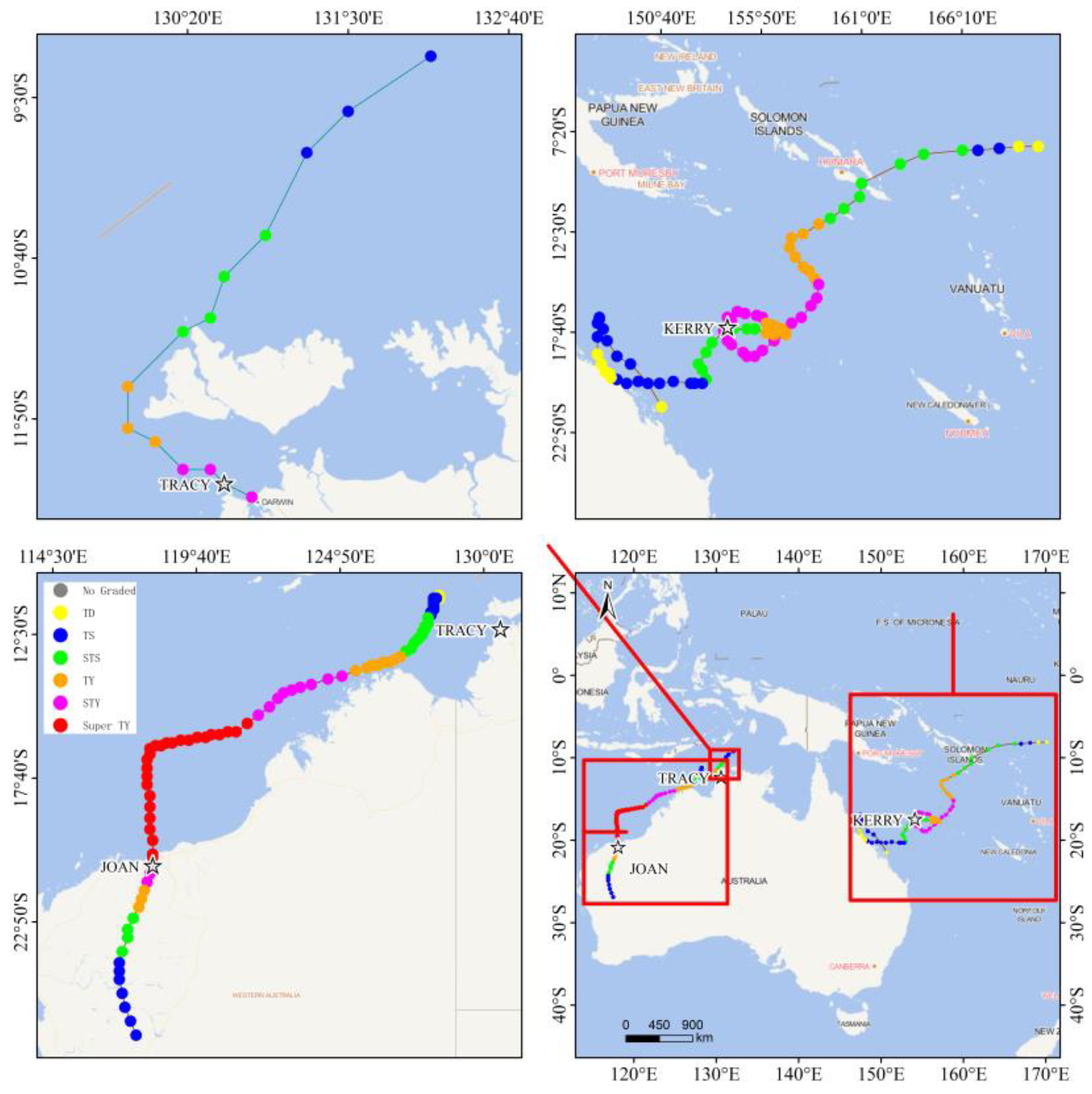
3.1. Australian Sea Area

We used the data from tropical cyclones Tracy (1974), Joan (1975), and Kerry (1979) that were previously utilized by Holland (1980) for his model. The tracks for these cyclones can be seen in Figure 1 (refer to Table 1). By substituting the data into Equations (16) and (17), we computed the two parameters A and B, respectively (refer to

Table 2. Presents the computed TC parameters for the Australian sea region.

	Parameters	A(16)	B(17)	Holland B	B(11)
TC
Tracy		1.0033	1.4821	1.5	1.4821
Joan		1.0420	1.0992	1.05	1.0983
Kerry		1.0322	1.4690	1.4	1.4682

). The Holland B data present in the table represent the B parameter values derived from Holland’s (1980) study. The value B(11) stands for the B parameter, calculated using Equation (11).

The three examined tropical cyclones originated in tropical waters around 10° S. As they evolved and progressed, they significantly affected the northwestern, northern, and northeastern coasts of Australia, respectively, within an impact range of 10° S to 30° S. We collected data from these three tropical cyclones [12,29] to assess the suitability of the two-parameter pressure model and wind field model in the Southern Hemisphere. We evaluated the model’s accuracy using the correlation coefficient (CC), mean absolute error (MAE), root mean square error (RMSE), and the Nash–Sutcliffe coefficient of efficiency (NSE).

Table 3. Analysis of pressure profile errors for tropical cyclones Tracy, Joan, and Kerry.

TC	Model	CC	RMSE	MAE	NSE
Tracy	Holland	0.992	3.069	2.358	0.968
	Fujita	0.986	4.535	3.523	0.931
	Takahashi	0.970	7.306	5.650	0.821
	Present model	0.992	2.967	2.281	0.971
Joan	Holland	0.998	2.804	2.400	0.978
	Fujita	0.994	6.050	5.623	0.899
	Takahashi	0.972	10.766	8.848	0.682
	Present model	0.999	2.172	1.966	0.987
Kerry	Holland	0.996	1.497	1.424	0.975
	Fujita	0.977	3.771	3.165	0.842
	Takahashi	0.929	7.714	6.681	0.338
	Present model	0.998	1.223	1.171	0.983

and

Table 4. Analysis of wind profile errors for tropical cyclones Tracy, Joan, and Kerry.

TC	Model	CC	RMSE	MAE	NSE
Tracy	Holland	0.936	5.079	4.024	0.760
	Fujita	0.910	7.040	5.722	0.539
	Takahashi	0.884	9.947	7.679	0.081
	Present model	0.936	5.153	4.109	0.753
Joan	Holland	0.921	5.668	5.012	0.266
	Fujita	0.925	4.190	3.587	0.588
	Takahashi	0.910	4.904	3.776	0.590
	Present model	0.920	6.285	5.633	0.100
Kerry	Holland	0.903	6.477	4.928	0.725
	Fujita	0.835	8.159	6.117	0.564
	Takahashi	0.685	11.441	10.418	0.142
	Present model	0.923	6.262	4.939	0.743

present the evaluation of the pressure and wind profiles’ accuracy.

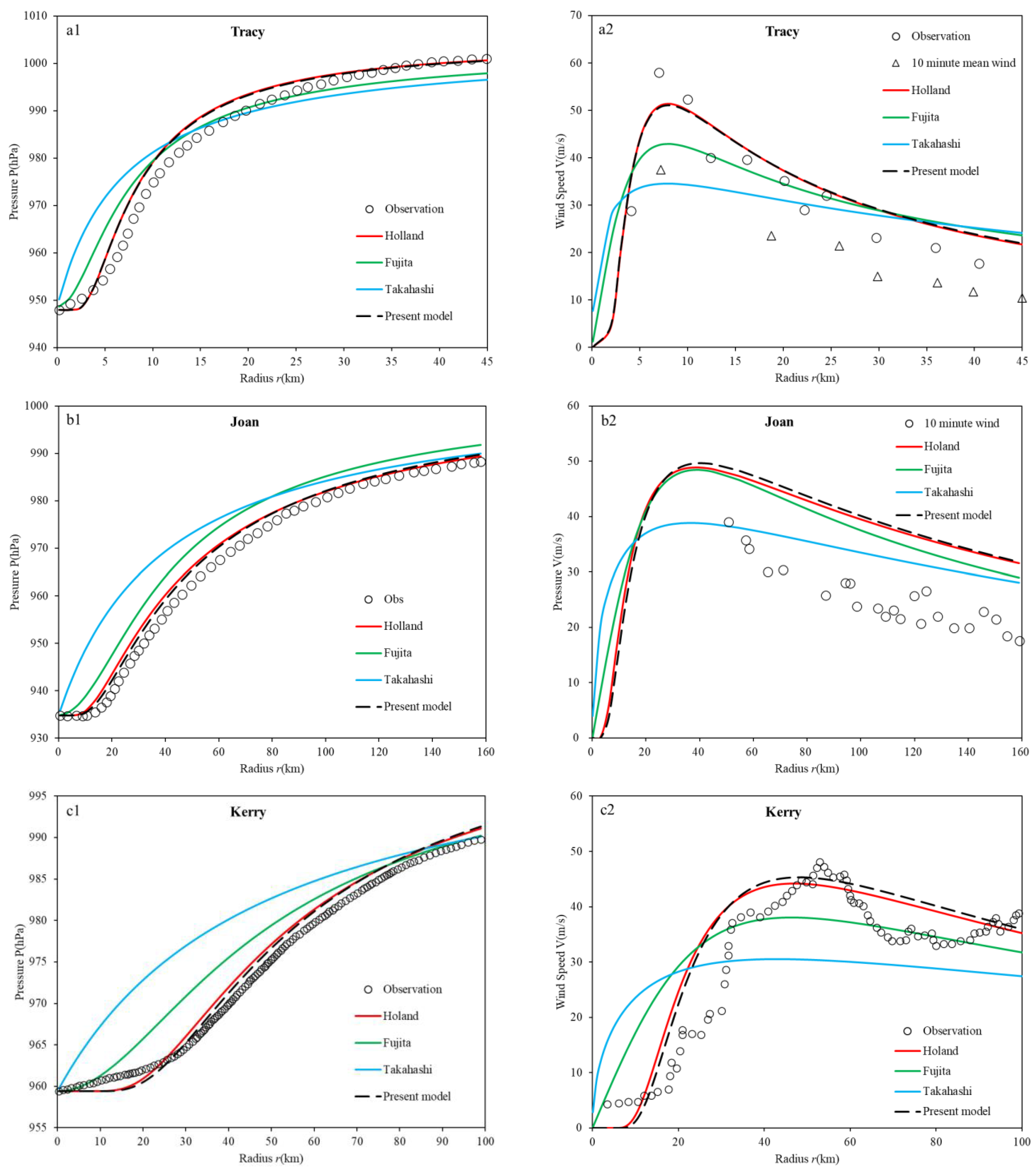
As depicted in Figure 2, the two-parameter model and the Holland model demonstrate close alignment with the measured data. In contrast, the Takahashi and Fujita models show less congruity. When the maximum wind radius is small (as in Tracy’s case with R = 8 km), the pressure profiles computed by the two-parameter model and the Holland model nearly converge. However, as the maximum wind radius increases (like Joan with R = 40 km and Kerry with R = 48 km), the pressure figures deduced by the two-parameter model are fractionally larger than those deduced by the Holland model. When the distance from the tropical cyclone’s center is under 2R, the Takahashi model provides larger pressure values than the Fujita model, but produces smaller values for distances exceeding 2R.

Holland’s literature [12] presents measured wind speed profiles for tropical cyclones Tracy and Joan as 10 min average wind speeds. For comparison, we used Harper’s conversion factor to apply a different time distance and translate the 10 min wind speeds to 1 min durations. The suggested conversion factor stands at 1.11 [32]. In Tracy’s case, the maximum wind speed calculated by the Fujita model aligns closely with the measured value after adjusting the time distance. The values estimated by both the two-parameter model and the Holland model exceed the measured value by 9.7 m/s, while the Takahashi model’s calculation falls short by 6.3 m/s. When juxtaposed with Tracy’s measured gust wind speed profile, both the two-parameter and Holland models overshoot the mark by 9.7 m/s. For Joan, the deduced wind speeds from the two-parameter model, the Holland model, and the Fujita model are largely in sync. When the distance from the cyclone’s center is less than the maximum wind radius, the two-parameter model estimates slightly larger values than the Holland model but smaller values than the Fujita model. At the approximate maximum radius, all three models show greater divergence. All computed values are larger than the measured wind speed by 6.9 m/s, 8.0 m/s, and 7.9 m/s, respectively, while the Takahashi model’s value is 1.7 m/s less than the measured value. For Kerry, all model calculations for the maximum wind speed radius render values smaller than the measured one, with the two-parameter model, Holland model, Fujita model, and Takahashi model estimating 0.8 m/s, 1.1 m/s, 7.4 m/s, and 15 m/s below the measured values, respectively.

In this study, p values less than 0.05 were deemed statistically significant. After determining the statistical significance between the current parameter model and various other models, the p value for all models in Tracy’s case exceeded 0.05. For Joan, only the Takahashi model obtained a p value under 0.05 (p = 0.044). In the scenario of Kerry, both Fujita and Takahashi models attained p values under 0.05 (p = 0.034 and p = 0.034, respectively).

The pressure error analysis in Table 3 indicates that both the two-parameter model and the Holland model exhibit correlation coefficients (CC) greater than 0.99, which surpass the scores of the Fujita and Takahashi models. The root mean square error (RMSE) and mean absolute error (MAE) values range between 1.2 and 3.1 m/s, lower than those of the Fujita and Takahashi models. The Nash–Sutcliffe model efficiency coefficients (NSE) values are approximately 0.97, exceeding the Fujita and Takahashi models. The two-parameter model slightly outperforms the Holland model in the pressure profile error analysis.

Table 4 presents the wind speed profile error analysis. During Tracy and Kerry tropical cyclone profile simulation, the wind speed profiles provided by the two-parameter and Holland models align more closely with the recorded wind speed profiles. Their CC is above 0.9, NSE is over 0.7 m/s, and both the RMSE and MAE are lower than the Fujita and Takahashi models. In the case of Joan’s wind speed profile simulation, the wind speed profiles formulated by the two model types better reflect the actual wind speed profiles. All models have CC values greater than 0.9, pointing to a high consistency with the observed values. Unlike the two-parameter model and the Holland model, the NSE is less than 0.3 m/s. During error analysis, we converted the 10 min average wind speeds using the recommended time-to-distance conversion coefficients. However, certain wind speed values from the collected data that fall below the maximum wind radius profile were missing. This led to lower average absolute errors than the Fujita and Takahashi models.

Yet, the NSE was small partly because of missing measurements, specifically those less than the maximum wind speed radius. The Fujita model represented a faster decrease in wind speed value following the maximum wind speed radius. Conversely, the Takahashi model had a relatively lower maximum wind speed value and a slower decrease after the maximum wind speed radius. This aligns more closely with the measured wind speed of Joan, thus allowing a better error accuracy evaluation of the Joan model than the two-parameter model and the Holland model.

In terms of wind speed, only the Takahashi model had p values less than 0.05, specifically p = 0.045 for Tracy, p = 0.007 for Joan, and p = 0.00054 for Kerry.

When comparing modeled values for pressure profiles and wind speed profiles, the estimates from the two-parameter model and the Holland model are substantially identical and congruent with the recorded data. These models offer a better fit than the Takahashi and Fujita models. Based on these findings, we suggest applying the two-parameter model to the Australian Sea region in the southern hemisphere.

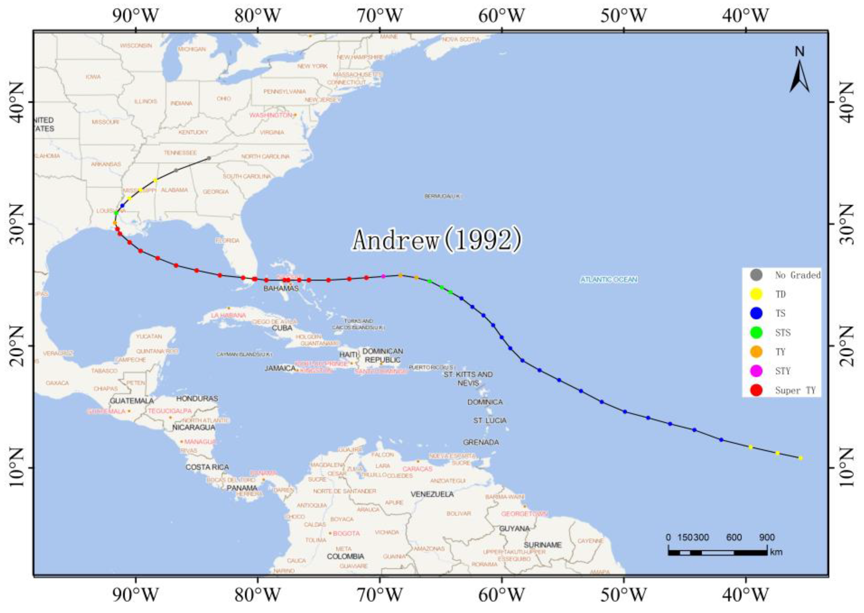
3.2. North Atlantic Sea Area

The North Atlantic Sea Area is also known for its tropical cyclone activity. For example, Tropical Cyclone Andrew in 1992, whose path is illustrated in Figure 3, severely impacted Florida, Louisiana, and the Bahamas, causing significant damage to the coastal areas (National Hurricane Center, NHC).

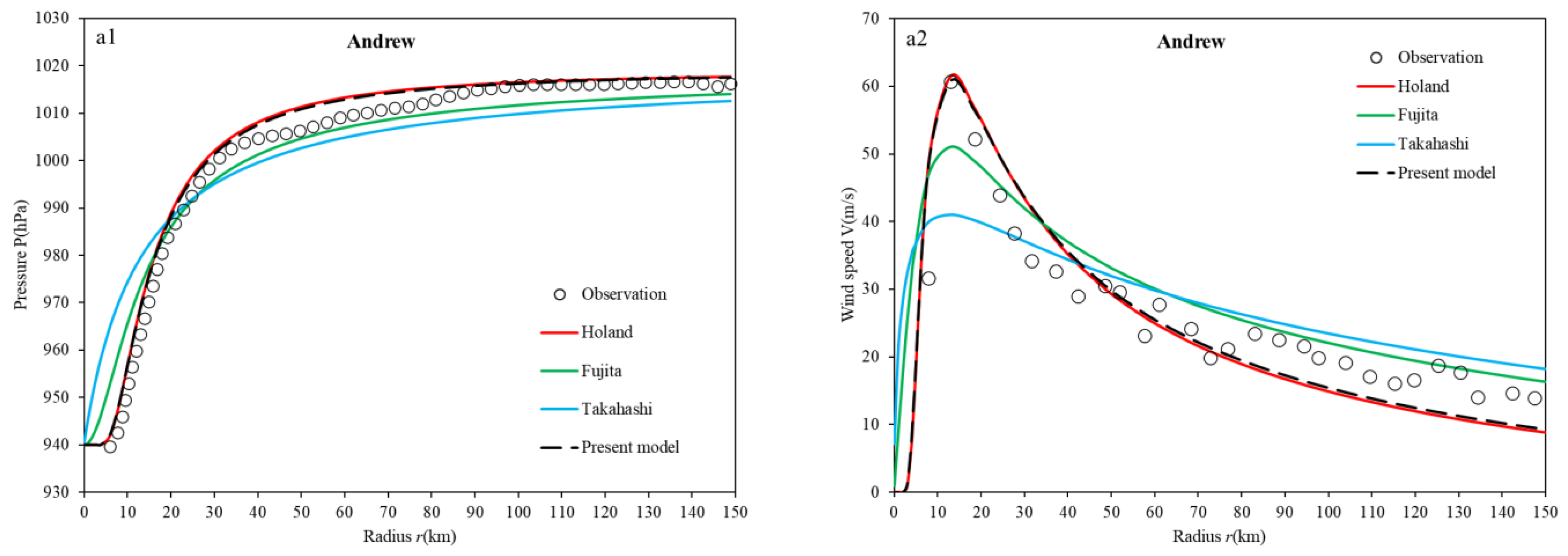
Willoughby [15] and Vickery [14] studied the pressure and wind profiles of tropical cyclones in the region. Figure 4 presents a comparison between the model-simulated values of these profiles and the recorded values. The parameters A(16), B(17), Holland B, and B(11) of Andrew’s Holland and two-parameter models, respectively, are 1.0093, 1.600, 1.7, and 1.6599.

Table 5. Error Analysis of Andrew’s pressure profile.

TC	Model	CC	RMSE	MAE	NSE
Tracy	Holland	0.998	3.365	2.951	0.978
	Fujita	0.996	5.910	4.481	0.934
	Takahashi	0.986	9.811	7.375	0.817
	Present model	0.999	3.076	2.639	0.982

and

Table 6. Error Analysis of Andrew’s wind profile.

TC	Model	CC	RMSE	MAE	NSE
Tracy	Holland	0.959	5.341	4.560	0.793
	Fujita	0.890	6.595	4.580	0.684
	Takahashi	0.834	7.593	5.580	0.582
	Present model	0.958	5.113	4.250	0.810

assess each model’s accuracy in representing Andrew’s pressure profiles and wind speed profiles.

In analyzing Andrew’s pressure profiles (Figure 4(a1)), the two-parameter and Holland models demonstrate a good agreement with the measured pressure profiles. When the distance from the cyclone’s center is less than the maximum wind radius (R = 13 km), the predicted pressure values of both the Takahashi and Fujita models are noticeably larger than the observed values. Conversely, the predictions made by the two-parameter and the Holland models are only slightly larger than the observed values. However, when the distance from the cyclone’s center is greater than the maximum wind radius (r > 22 km), the predicted values of the Takahashi and Fujita models are smaller than the observed values. Here, the predictions of the two-parameter model slightly outperform those of the Holland model.

Regarding Andrew’s wind speed profile (Figure 4(a2)), at the maximum wind speed radius, the Holland model’s estimated wind speed is 0.8 m/s larger than the measured speed. The two-parameter model’s predictions align with the measured speed, whereas the estimated values of the Takahashi and Fujita models fall short by 19.7 m/s and 9.7 m/s, respectively. When the distance from the cyclone’s center exceeds 80 km, the Takahashi model overestimates the wind speed. At this greater distance, the Takahashi, Fujita, and two-parameter models predict wind speeds that exceed, are between, and fall short of the measured values, respectively. The Holland model’s predictions are somewhat lower than those of the two-parameter model and the measured values.

The p values for the Holland, Fujita, and Takahashi models applied to Andrew each exceed 0.05.

From the error analysis of Andrew’s pressure profile in Table 5, it is evident that the correlation coefficients, root mean square error (RMSE), mean absolute error (MAE), and Nash efficiency coefficient of both the two-parameter and Holland models outperform those of the Fujita and Takahashi models across these four metrics. Further, the two-parameter model marginally surpasses the Holland model. The Holland model exhibits superior correlation coefficients and Nash efficiency coefficients than the Fujita and Takahashi models, while the RMSE and MAE of all four models are relatively comparable. Notably, only the Takahashi model’s p value is less than 0.05 (p = 0.024).

To summarize, the two-parameter and Holland models demonstrate stronger applicability when compared to the measured pressure and wind speed profiles, outperforming both the Takahashi and Fujita models in the Andrew case study. Predictions of pressure and wind speed profiles by the two-parameter and Holland models are nearly identical, with an impressive ability to accurately reproduce the observed measurements. As such, the two-parameter model is also well suited for application in the North Atlantic Ocean.

3.3. Western North Pacific

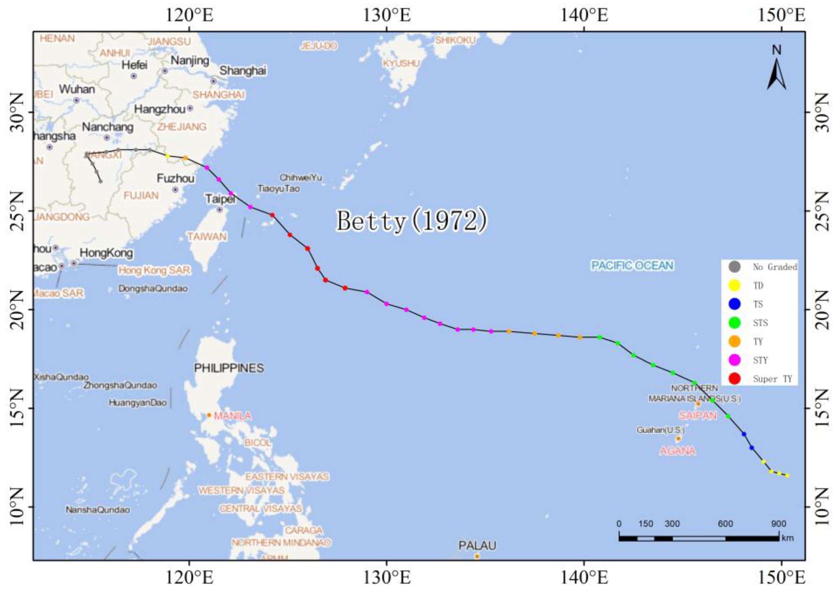
Approximately one-third of the world’s tropical cyclones occur in the Western North Pacific (WNP). In 1972, Tropical Cyclone Betty made landfall in the southern area of China’s Zhejiang Province, leading to casualties and property damage in the coastal regions of Zhejiang and Fujian. This has made Betty a model case for studying cyclones in the WNP (refer to Figure 5). Track information regarding Tropical Cyclone Betty was acquired from the China Meteorological Administration (CMA), while the pressure and wind speed profile data were sourced from the Annals of Tropical Cyclones [33] and the research literature by Zhong [31]. 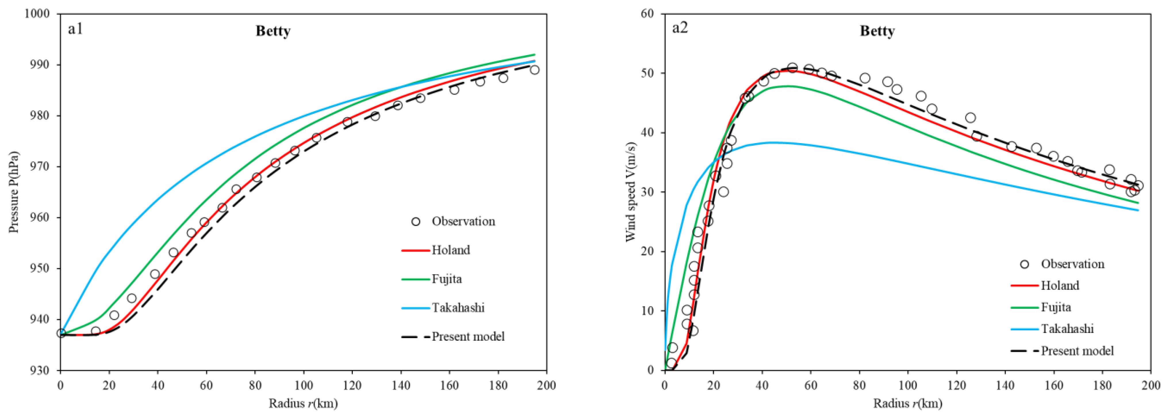Figure 6 portrays the comparison between the simulated and measured values associated with the pressure and wind speed profiles of Betty. The parameter values A(16), B(17), Holland B, and B(11) for Betty’s Holland and two-parameter models are, respectively, 1.0796, 1.1855, 1.16, and 1.1821.

Referring to the pressure profiles of Betty (Figure 6(a1)), it is evident that the pressure values calculated by Takahashi and Fujita are higher than the measured ones. Yet, the Fujita model yields calculations closer to the observed values than the Takahashi model, with a radial shift pattern that essentially mirrors that of the observed values. In the two-parameter model, calculated pressures are less than measured values within 100 km from the cyclone center but exceed those measurements beyond 120 km. Conversely, the Holland model generates slightly lower pressure than the measurements within a 60 km radius from the cyclone center, but it aligns best with those measurements between 60 km and 120 km. Beyond 120 km, the Holland model results in higher calculated values compared to measurements.

On the matter of wind speed, Figure 6(a2) illustrates the wind profile taken for Betty at 02:00 on 17 August 1972, with its center position at (122.1° E, 25.9° N). The central pressure recorded was 937 hPa and the peak wind speed was 50 m/s, as evidenced by CMA’s optimal path data. The CMA’s reported maximum wind speed was utilized as the assessment criterion, resulting in an equal rescaling of the wind speed profile. From this profile, it is clear that both the two-parameter and Holland models accurately replicate Betty’s wind speed profile. However, wind speed calculations from Fujita and Takahashi models are initially higher and subsequently lower than measured values. Lastly, the p values for all models are found to exceed 0.05.

The error analysis for both pressure and wind speed profiles, as presented in

Table 7. Pressure profile error analysis of Betty.

TC	Model	CC	RMSE	MAE	NSE
Tracy	Holland	0.999	1.375	1.172	0.993
	Fujita	0.999	3.275	3.168	0.961
	Takahashi	0.973	8.659	7.177	0.724
	Present model	0.998	2.121	1.694	0.983

and

Table 8. Wind profile error analysis of Betty.

TC	Model	CC	RMSE	MAE	NSE
Tracy	Holland	0.981	2.983	2.259	0.953
	Fujita	0.942	5.407	4.577	0.846
	Takahashi	0.745	10.686	9.366	0.399
	Present model	0.984	3.289	2.173	0.943

, suggests that the two-parameter model and the Holland model have analogous accuracies. These models exhibit values surpassing 0.98 and 0.94, respectively, which outperform those generated by the Fujita and Takahashi models. Furthermore, it is noteworthy that the p values for all of these models exceed 0.05.

3.4. Overall Accuracy Assessment

On evaluating the respective accuracy of five tropical cyclones from three sea areas, it is evident that the simulation accuracies of the two-parameter model and Holland model, for both pressure and wind fields, mirror each other. Both models outperform the Fujita and Takahashi models. In a bid to delve deeper into the strengths and weaknesses of these respective simulation accuracies, the analyzed data collected from the five tropical cyclones and the corresponding model computation results were combined. The computed accuracy indices, as reflected in

Table 9. Overall error analysis of tropical cyclone profiles.

Model	CC	RMSE	MAE	NSE
Holland	0.996	2.407	1.979	0.985
Fujita	0.989	4.712	3.852	0.943
Takahashi	0.973	8.659	7.045	0.806
Present model	0.996	2.048	1.604	0.989

and

Table 10. Overall error analysis of tropical cyclone wind speed profiles.

Model	CC	RMSE	MAE	NSE
Holland	0.853	11.156	5.533	0.844
Fujita	0.805	11.384	6.082	0.838
Takahashi	0.637	14.462	8.690	0.738
Present model	0.864	11.158	5.421	0.846

, will provide further insights.

The error analysis of pressure profiles depicted in Table 9 indicates that the two-parameter model’s accuracy slightly surpasses the Holland model, with the latter significantly outperforming the Fujita model. The Takahashi model yields the least accuracy. Albeit the overall errors of the wind speed profiles somewhat reflect the pressure profiles’ pattern, the discrepancies are not as remarkable. The two-parameter model’s CC, MAE, and NSE statistics are marginally superior to the Holland model, with a slightly reduced RMSE. However, for the Fujita model, its accuracy is relatively less compared to the two-parameter and the Holland models, but with insignificant differences. The accuracy indices for the Takahashi model is markedly lower than the other three models. A comprehensive analysis of these four models across five tropical cyclones in three sea areas reveals that the two-parameter model and Holland model have minor differences in their computations of pressure and wind speed compared to the two-parameter model and Fujita model. Furthermore, the two-parameter model’s accuracy and agreement with the actual measured values are superior. Thus, the two-parameter pressure model proposed in this paper boasts of high applicability and accurate results, making it suitable for analyzing tropical cyclones.

3.5. Spatial Wind Validation with Reanalysis Data

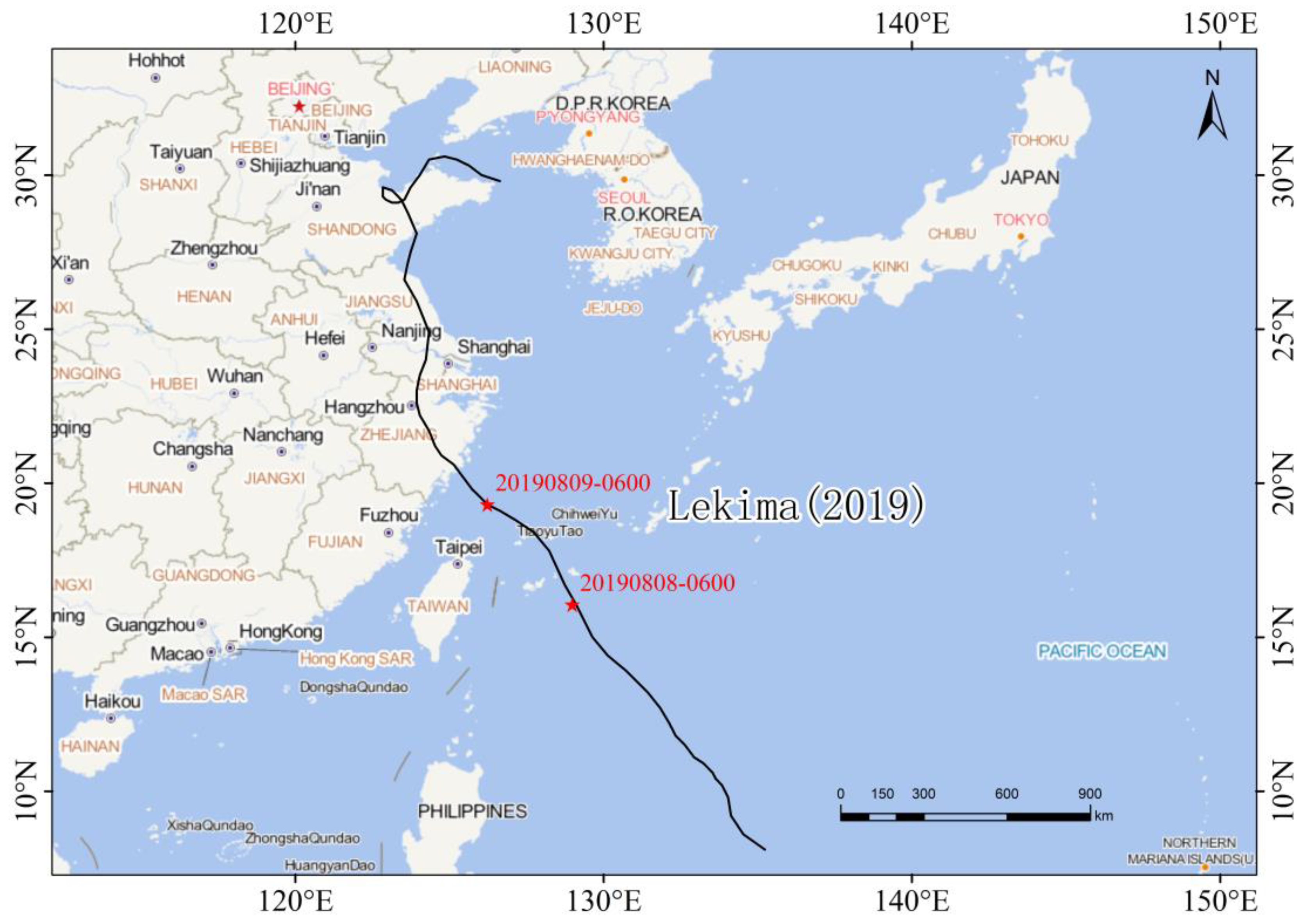
Typhoon Lekima, as depicted in Figure 7, originated on the 4 August 2019 at 0600 UTC and ultimately dissipated on the 13 August 2019 at 0300 UTC. It made landfall near Taizhou, China, registering winds clocking at about 48.6 m/s. The typhoon induced severe rains and gusty winds along the coast of the Zhejiang province, causing widespread damage. With a death toll surpassing 66, it affected over 14 million people and resulted in thousands of homes demolished. The total economic damages are estimated to be around CNY 52 billion (around USD 8 billion) [34].

For an in-depth analysis, wind speed data during the Lekima period were extracted from the ERA5 reanalysis data at two instances: at 0600 UTC on the 8 August 2019 and at 0600 UTC on the 9 August 2019. The data were sampled from the center of the typhoon to the four quadrants (N-S, W-E, NW-SE, NE-SW) within a radius of 400 km. The China Meteorological Administration (CMA) provided maximum wind speeds of 55 m/s and 48 m/s for the two instances. The expressions proposed by Willoughby et al. [35] were used to obtain the maximum wind radii for the two instances at 30 km and 35 km, respectively. For the first event, A(16) was 1.0267 and B(17) was 1.1481, while for the second, A(16) was 1.0426 and B(17) was 1.0795.

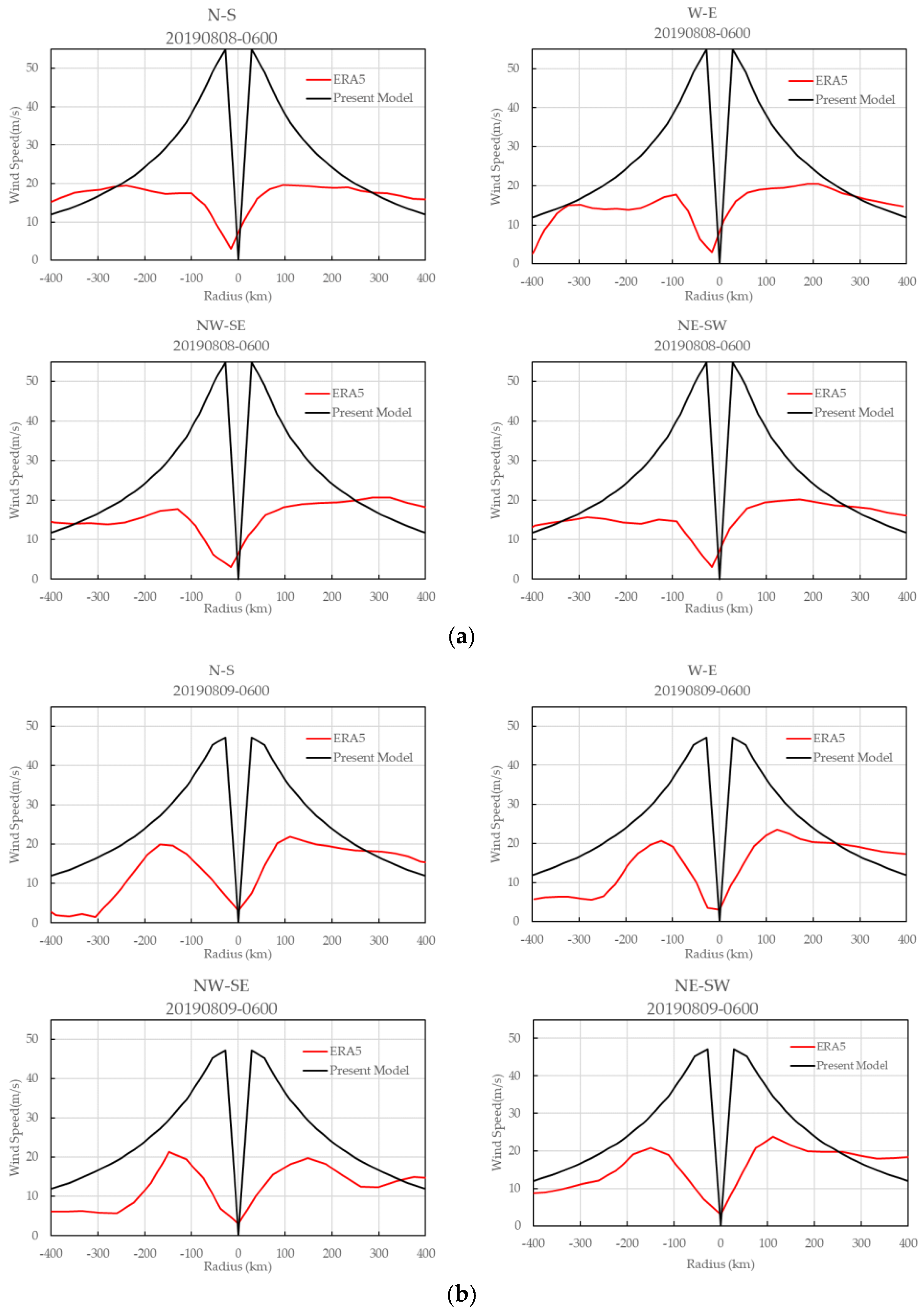
Upon comparing the computed values of the two-parameter model with reanalysis data in Figure 8, the following insights can be drawn: (1) The reanalysis data significantly underestimate the wind speeds of the tropical cyclone near the radius of maximum wind speed. (2) As the distance increases, the wind speeds calculated by the model decay more rapidly. (3) The wind speeds on the island’s side decay faster than those on the sea side when impacted by larger islands or landmass, due to friction. (4) The circularly symmetric wind field fails to accurately represent the actual wind field, which can be improved by superimposing the moving wind field. (5) The model wind field offers better accuracy in high-speed wind areas near the center of the tropical cyclone, as well as far away from these areas.

The two-parameter model successfully replicates the characteristics of the wind field near the tropical cyclone’s maximum wind speed. A comparison with the ERA5 reanalysis wind field shows that the hybrid wind field, which combines the model wind field and the reanalysis wind field, more accurately recreates the actual wind field of the tropical cyclone.

4. Conclusions

In this research, the initial step involved procuring the gradient wind equation from the fundamental assumptions of the wind field model. Post theoretical derivation, it was concluded that the Holland model does not comply with the derivative equation of the gradient wind. This led to the proposal of an improved two-parameter pressure model specifically for tropical cyclones. The validation of this two-parameter pressure model was accomplished by applying measured pressure and wind speed profiles of five tropical cyclones across three different marine regions, and comparing the outcome with widely recognized models such as Holland, Fujita, and Takahashi.

This study offers a mathematical resolution to the deficiencies of traditional pressure models. An error analysis revealed that the presented two-parameter pressure model is more accurate than the Holland, Fujita, and Takahashi models and handles the issue of traditional models not adhering to the gradient wind derivative function equation. Equations (16) and (17) further facilitate convenient usage of parameters A and B of the two-parameter model. Moreover, the features of this model have been discussed.

From a statistical standpoint, the outcomes of the two-parameter model do not present a significant deviation from the results of the Holland and Fujita models. However, a statistically significant disparity exists with the results of the Takahashi model.

This study encompassed the collection of five pressure and wind speed profiles of tropical cyclones. Future studies should focus on gathering more reliable profiles for validating the two-parameter model.

Comparative analysis indicates that a hybrid wind field, which integrates modeled and reanalysis wind fields, is one of the superior methods for reconstructing the wind field of tropical cyclones.