1. Introduction
The ice covering Arctic shipping routes is constantly broken up into numerous floating ice floes, which damages the hull of the vessels that operate in these waters. Such ice-floe fields are generally considered the most important challenge for Arctic shipping. This has motivated various studies on the interaction between marine vessels and ice floes. Particularly, the floes can induce not only significant resistance on the ship but also impact forces on the hull surface. Therefore, predicting the effect of ice-induced collision is crucial. Considering the high costs of experimental analyses and the shortage of field-measurement data, numerical models offer a cost-effective means to investigate the effect of ice floes on vessels. Since damage to ships operating in the Arctic route causes severe environmental and property problems, the structural capacity of vessels against ice collisions must be assessed at the design stage. Therefore, various studies have conducted structural safety assessments to determine the effects of environmental loads on ships. In particular, these studies (e.g., Fabrice et al. [
1]; Riska et al. [
2]; Adumene et al. [
3]) have assessed the effects of cargo load, wave load, and harsh fluid impact applied to a ship, and the evaluation procedures have been curated by shipping classification societies [
4,
5,
6,
7]. For ships operating in Arctic regions, collisions caused by ice floes are the most important risk. Nonetheless, few efforts have been made to assess the impact of drift ice on both the impact load and structural safety of Arctic vessels. The ice impact load can be inversely estimated based on the reactive stress measured on a ship operating in a specified route. However, the measured data can only be used to estimate the impact load in a specific route. Therefore, the ice impact load measured on the ship can be applied only to ships that have a similar hull form and operate in the same route. Therefore, many attempts (e.g., Gao et al. [
8]; Kim et al. [
9]; Liu et al. [
10]; van den Berg [
11]; Sun and Shen [
12]) have been made to predict ice impact loads and evaluate the impact resistance of the hull using numerical analysis to contribute to Arctic ship design.
Vessels operating in Arctic routes experience various types of damage from interactions with drift ice. The type of hull damage is related to the magnitude of the impact energy of the drift ice. When a ship collides with a large fragment of drift ice at high speed, the hull completely collapses. An ice impact with small energy may cause localized hull damage and deformation. Even if the collision energy induces stresses below the yield stress, repeated ice collisions may cause fatigue damage or wear damage to the hull. Vessels operating in Arctic routes with abundant drift ice experience continuous frictional forces as they advance while resisting the drift ice. Once the coating is separated from the hull surface by frictional force, the wear load caused by friction begins to accumulate on the surface of the hull plate. Afterward, wear damage due to abrasive force, which peels off the steel of the hull, spreads out onto the hull surface. The accumulated abrasion of the hull plates can eventually cause corrosion damage, in addition to deteriorating the structural strength of the hull. Various theoretical approaches and shipping classification criteria have enabled the analysis of structural stress and deformation response due to ice impact (Kwon et al. [
13]; Nho et al. [
14]). However, very few studies have actively sought to predict the wear damage of the hull due to ice impact.
The purpose of this study was to develop a numerical model to enable the estimation of the wear of a vessel hull undergoing collision with drift ice based on three key considerations. The first consideration is the influence of the sea environmental load in the Arctic route on the ice floes. Given that both vessels and ice floes are subjected to Arctic environment loads during their lifetime, the numerical model would also have to reflect the hydrodynamic behavior of drift ice. The second consideration is the behavior of ice floes continuously experiencing fluid flow and their interactive loads. The behavior of ice fragments can be expressed by solving a multi-phase problem consisting of a fluid phase, which numerically represents the environmental load, and a particle phase, which represents the motion of the ice fragments. The last consideration is the development of a reasonable wear assessment method. Since wear is caused by continuous contact friction between the ice fragments and the hull surface, it can be simulated by a contact element in the FEA. However, FEA including contact elements is a typical nonlinear problem, which not only demands large computation times but also cannot easily render a stable converging solution. In addition, it is practically impossible to set a contact condition by predicting the behavior of a large number of irregular flowing ice. In this study, we discuss the three aforementioned considerations and present a numerical implementation procedure for predicting abrasive wear damage on hull surfaces subjected to cumulative ice impact. Previous studies have attempted various numerical methods to predict hydrodynamic loads and the behavior of floes in the Arctic environment. These studies are mainly aimed at predicting hull resistance and impact loads due to interaction with floes, but they do not address the impact on the wear of the hull. In most studies, the geometry of the floe was simplified to a spherical or cylindrical shape to make the calculation of contact forces more manageable. As a result, they did not account for the effects of the geometric features of the floe on the structural response, resistance, and impact loads. Numerical algorithms for wear, which refers to damage from prolonged operation characterized by continuously changing structural boundary conditions, are particularly challenging to present. To improve wear prediction, a numerical model must account for the shape of the floe and changes to the hull boundary caused by material loss due to wear. This requires overcoming limitations of existing studies and establishing a comprehensive model. However, the implementation of numerical analysis is focused on reflecting physical characteristics rather than quantitatively accurate predictions of wear. The effects of hull shape, operating conditions, and wear-inducing material properties that affect wear are not covered in this study.
2. State of the Art
Studies on the structural safety of vessels operating in Arctic routes have been conducted in terms of the dynamic material properties of ice, the motion of ice floes, impact forces and friction loads, and structural responses. Han et al. [
15] conducted a compression test of conical ice specimens to obtain the strain–load relationship. Additionally, the load–displacement relationship of the conical ice predicted by the FEA was compared with the experimental results. By applying this relationship to FEA, the spalling of ice under the crushable compression was simulated. Cai et al. [
16] and Zhu et al. [
17] estimated the dynamic stress–strain relationship of steel and ice using the Cowper–Symonds model and the Crushable Foam model, respectively. The authors demonstrated that the dynamic material properties of both steel and ice can be applied to FEA to predict the fracture shape of ice subjected to impact.
The estimation of ice impact loads requires an a priori knowledge of the ice floe motion, which represented the first major concern of the present study. Kim et al. [
18] modeled the behavior of a ship, drift ice, and seawater using the arbitrary Lagrangian–Eulerian (ALE) technique and calculated the ship resistance using FEA. The ice resistance of the icebreaker was measured and compared with that of ALE-based FEA by conducting an ice-breaking towing test in the ice basin. The authors ultimately aimed to calculate the ice resistance of the icebreaker. An alternative approach to FEA is to couple computational fluid dynamics (CFD) with a particle model such as the DEM (discrete element method) or SPH (smoothed particle hydrodynamics), which allows for fully non-linear solutions including complex geometries to investigate structure–flow–ice interactions. In other words, CFD and DEM have been coupled to model ship–flow–ice interaction. Robb et al. [
19] presented a SPH-DEM coupling model to numerically simulate the behavior of an ice floe on a free surface. Moreover, Huang et al. [
20] constructed a CFD model to calculate the ship resistance in response to ice collision. The flow generated by the operating vessel was calculated using CFD, and the behavior of the drift ice was simulated by adding pancake ice to the flow field. Liu et al. [
21] also performed CFD-DEM coupling analysis to evaluate hull resistance by accounting for the motion of ice floes. By assuming that the drift ice particles were spherical, a CFD-DEM model was used to predict the hull resistance applied to the vessel. The authors tested both one-way and two-way coupling schemes in the CFD-DEM model and calculated the velocity and pressure of ice particles experiencing the flow of surrounding sea water. Their results demonstrated that the two-way coupling analysis could simulate the motion of the ice floe more accurately than one-way analysis. However, the result of the one-way coupling method was estimated to be only approximately 5% different from the two-way coupling analysis. Therefore, although the two-way coupling method provides estimates that are close to experiment-derived values, it should be noted that it takes more computation time than the one-way coupling method. Therefore, the authors suggested that the one-way coupling method can be practical. Particularly, as the ship moves at a lower speed, the difference in simulated results according to the coupling method becomes smaller, and the one-way coupling provides a more conservative result from the perspective of impact forces. Therefore, the one-way coupling method may be more reasonable for predicting wear generated at low-velocity impacts. Liu et al. [
22] and Zhang et al. [
23] also simulated the behavior of ice floes surrounding a moving ship by coupling CFD and DEM. Particularly, CFD was applied to simulate the fluid surrounding the ice floes, whereas DEM was incorporated to account for the ice motions and ship-to-ice or ice-to-ice collisions. By integrating these approaches, the proposed method could account for the influence of ship-generated fluid flow on the ship–ice interactions.
Table 1 summarizes the methods and assumptions of several references that utilized numerical simulations to analyze the behavior of drifting ice. Notably, these references employed a highly simplified representation of the ice floe geometry which affects hull wear. In this study, the numerical model reflects the ice floe’s geometry as accurately as possible, resembling its real shape. Also, while the references aim to estimate the resistance and impact loads due to ice impact, this study evaluates the hull’s wear damage from ice impact.
The hull damage caused by large icebergs in high-speed collisions is not much different from ship-to-ship collision in terms of structural deformation caused by the excessive collision energy, except that the colliding object is ice and the behavior of ice should be predicted. Suyuthi et al. [
24] developed a probability model that assesses the collision loads of ice with various thicknesses and velocities. Cho et al. [
25] investigated the wear of hull coatings through ice friction experiments. Changes in the coated surface of the hull were measured by varying the friction force, surface roughness, and coefficient of friction. Kietzig et al. [
26] summarized the friction coefficient of ice collected by relevant studies and presented the factors that affect the friction force of contacting ice, including ice temperature, sliding speed, and vertical load. The main purpose of this study is to determine the effect of various external factors on the friction of ice. Several other studies have also applied FEM to wear assessment (Shimizu [
27]; Xie [
28]). However, the applicability of FEM for the evaluation of wear caused by contact between metal planes is limited and the wear force of impacting particles cannot be easily accounted for when using this model. Chen et al. [
29], Xu et al. [
30], and Zhang et al. [
31] suggested that the friction behavior derived from the interaction between fluid and solid particles could be efficiently predicted by applying the CFD-DEM coupling method. Walker et al. [
32] also demonstrated that the particle shape has a great influence on wear through several friction experiments. Huang et al. [
20], Luo et al. [
21], Zhang et al. [
23], and Shunying et al. [
33] analyzed the collision between the hull and the ice floe by coupling CFD and DEM. However, they simulated the collision of the ice floe with the hull by assuming that the ice particles were spherical and free shapes were obtained by combining several spherical particles. Therefore, their study could not efficiently reflect the wear caused by sharp edges or vertices of ice particles. When the surface geometry of the impact object changes due to wear, the flow of the colliding particles changes. Furthermore, as the particle flow changes, regions with high wear energy shift non-linearly. Shunying et al. [
33] analyzed the effect of changes in the geometry of the worn surface on particle flow and the effects that these variables had on the final wear pattern. However, to the best of our knowledge, no previous studies have examined the effects of the changes in the hull shape due to collision-induced wear on ice flow and ductility.
Our study sought to develop a numerical model to evaluate the wear of a vessel hull by considering the particle shape and changes in the particle motion due to wear-induced changes in the shape of the impacted object. Finally, this study presents a practical approach for the estimation of Arctic ship wear, which could be used as a basis for the design of safer and more resilient Arctic vessels.
Table 1.
The summary of reference studies which evaluate floe behavior on the fluid flow of the route.
Table 1.
The summary of reference studies which evaluate floe behavior on the fluid flow of the route.
| Author | Numerical Scheme | Floe Shape | Purpose |
|---|
| Kim et al. [18] | ALE-based FEA | Rectangular box | - Evaluating the ice resistance of the icebreaker
- The ice resistance of the icebreaker was measured and compared with that of ALE-based FEA |
| Robb et al. [19] | SPH-DEM | Sphere | - Simulating the behavior of an ice floe on a free surface |
| Huang et al. [20] | CFD-DEM Coupling
(DEM embedded in CFD) | Pancake | - Evaluating the ship resistance in response to ice collision |
| Liu et al. [21] | CFD-DEM Coupling
(DEM embedded in CFD) | Spherical | - Evaluate hull resistance by accounting for the motion of ice floes
- Comparing one-way and two-way coupling schemes in CFD-DEM coupling |
| Zhang et al. [23] | CFD-DEM Coupling
(DEM embedded in CFD) | Glued sphere | - Simulate the behavior of ice floes surrounding a moving ship
- Compare results from experiments and analysis
- Analyze how variable settings affect analysis results in numerical simulations |
| Shunying et al. [33] | CFD-DEM Coupling | Pancake | - Evaluating the ice impact loads under different operating conditions |
4. Evaluation of Hull Wear Due to Collision with Ice Floes
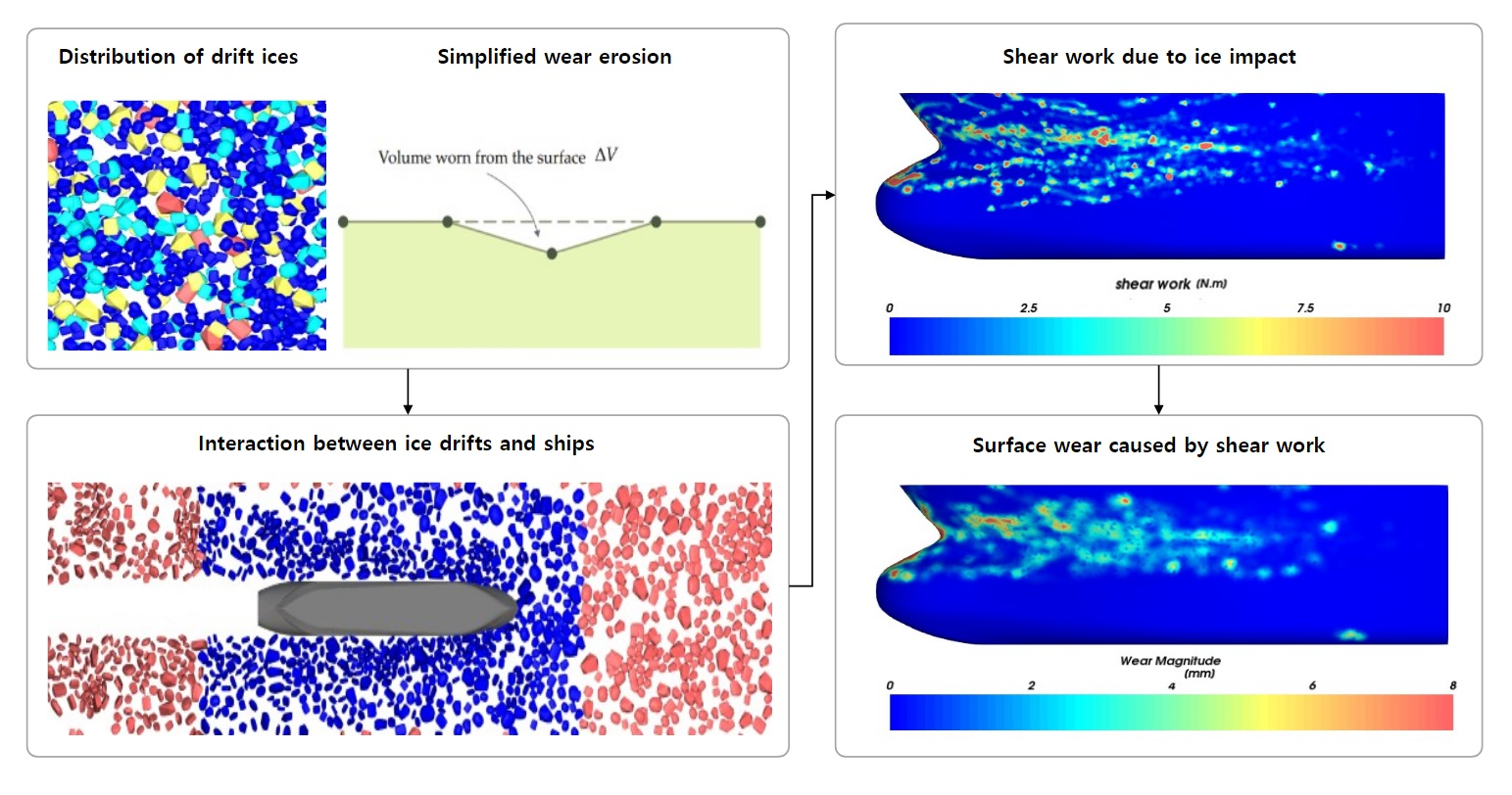
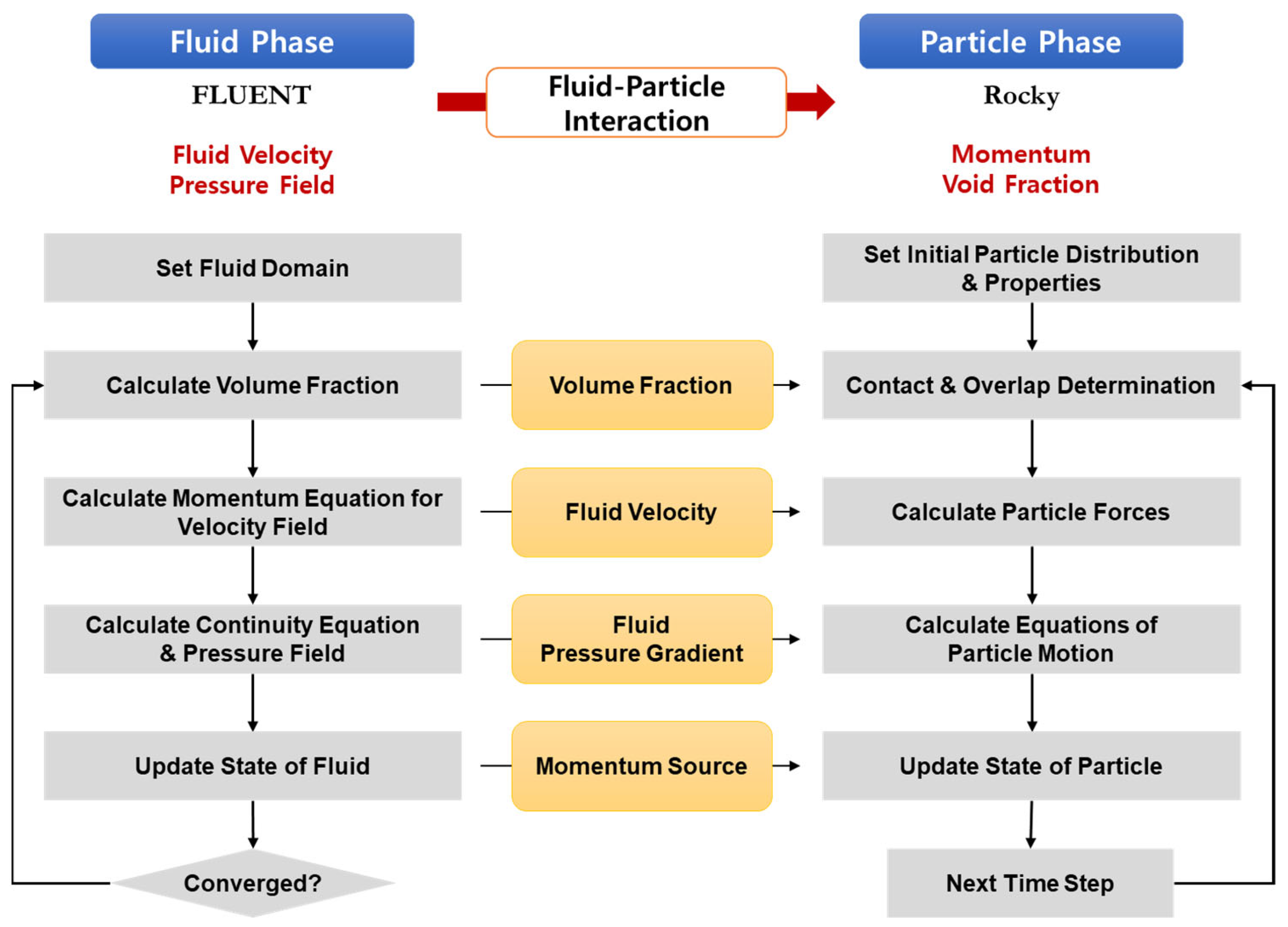
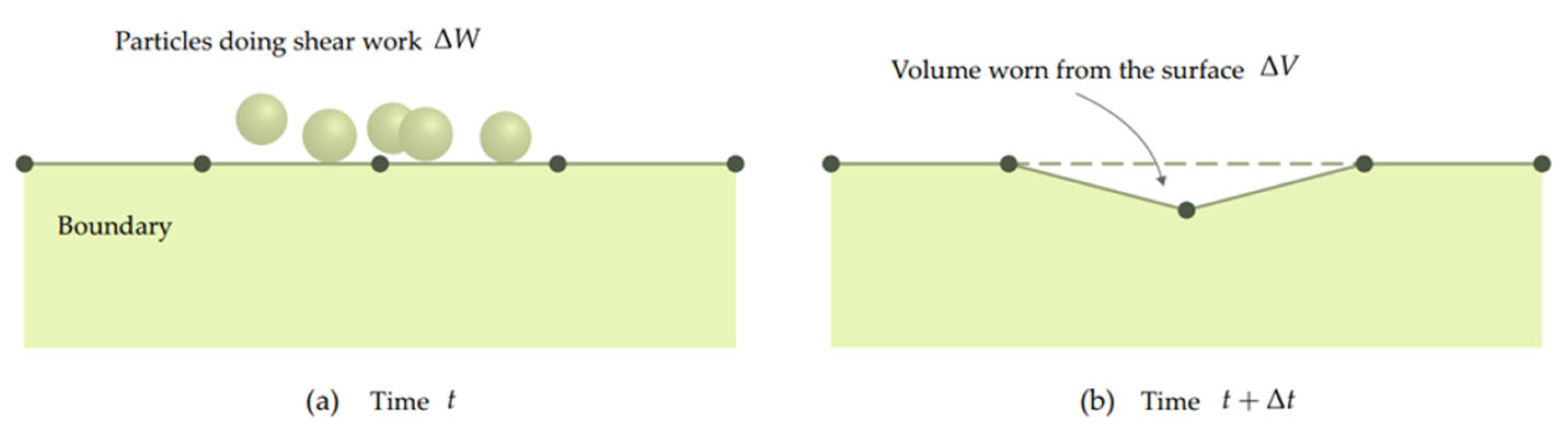
To evaluate the wear of Arctic operating vessels in ice floes, multi-phase problems consisting of particles and flow can be solved numerically. In this study, the flow of the sailing route was modeled as a fluid phase, whereas the behavior of the ice floes was modeled as a particle phase. The fluid flow of the route acts as a dominant load on the ice floes but the behavior of the ice floes does not have a significant effect on the fluid flow on a ship’s route. To reflect these behavioral characteristics, the one-way coupling method is reasonable. The fluid phase acts as the load of the particle phase, and the hull is defined as the boundary condition. The hull wear is evaluated by extracting the load component that causes wear from the impact energy generated in the particle phase. Hull wear due to collision with particles was evaluated by applying the Archard wear law, which is defined based on shear work and the volume loss ratio.
Wear is a failure that occurs when energy is continuously transferred from ice floes to the hull surface over a long period of time. Therefore, it is impossible to evaluate wear on a real-time scale and over an operational distance. To overcome this limitation, a method for numerically accelerated analysis is needed. Considering the characteristics of wear, it has been shown that wear can be efficiently predicted by converting long-term loads into equivalent material constants. In Lee et al. [
41], the specimen was moved 208 km for 20 h in the experiment, while in the numerical model, the wear was evaluated by moving 3 m in 1.18 s with the same specimen geometry and travel speed. Although the analysis was accelerated, the wear shape could be accurately predicted. In equation (25), the amount of wear volume per unit time is defined as the product of the material constant and the shear work accumulated per unit time. The material constant
is defined as the volume lost due to the accumulated shear work per unit time. If
is increased by
times, there is an effect of increase in the unit time, as shown in Equation (26).
where
is enlarged material constant for accelerated analysis,
is actual material constant and N is enlargement factor.
is defined as shear work accumulated over
N times the unit time. Through this relationship, micro material loss cannot be evaluated, but it can be evaluated from a macro perspective. If the
of a material with a
of 1 m
3/J was defined as 100 m
3/J, then
is 100. According to Equation (26), shear work accumulated for 1 s of simulation time can be evaluated as shear work accumulated for 100 s of real time by
. Therefore, the volume of wear loss that occurred for 100 s can be evaluated through the 1 s analysis result.
N can be determined according to the acceptable analysis time and how much micro material loss can be tolerated. The purpose of this study is to develop a numerical model for assessing wear in ships traveling Arctic routes. The shape of ship, operating conditions, and wear-inducing material properties were not of primary interest in this study. Therefore, the wear magnitude evaluated in this study is not representative of actual operational ships.
4.1. Evaluation Conditions
In the early stages of operation, the painted hull surface is damaged by friction with the floating ice. Since the shape of the hull does not change, there is no need to account for the shape change due to wear. If the operation is prolonged, friction with the ice floe accumulates and the material of the hull is lost. Since the shape of the hull changes due to material loss, the shape change due to wear must now be accounted for. Evaluation models suitable for each situation were thus presented. The evaluation was conducted assuming a scenario in which a vessel sails 200 m on a route with ice floes. To calculate the fluid force of the route, an evaluation model was constructed with Ansys Fluent. It was assumed that there was no seawater flow, and the buoyancy force was considered by implementing the pressure gradient of the fluid force. To simulate buoyancy and conditions in which there is no fluid flow, an arbitrary speed was applied upward from the lower part of the CFD model and analyzed, after which the speeds in all directions were patched to 0. The velocity in all directions was fixed to 0 to prevent particle movement due to seawater flow, and the depth direction pressure gradient was implemented to define the buoyancy force. The results of CFD analysis were applied as the load of DEM analysis. For the coupling of CFD and DEM, the Ganser drag law was applied to calculate drag force. The density of water was defined as 1000 kg/m3 and the viscosity as 0.001003 kg/m−s.
Transport Canada [
46], a Canadian company that operates through the Arctic Ocean, suggests a range of safe operating speeds to avoid potential accidents from ice collision. Therefore, our evaluations were carried out based on the safe speeds of 4, 6, and 10 knots suggested by Transport Canada (AMNS) [
46].
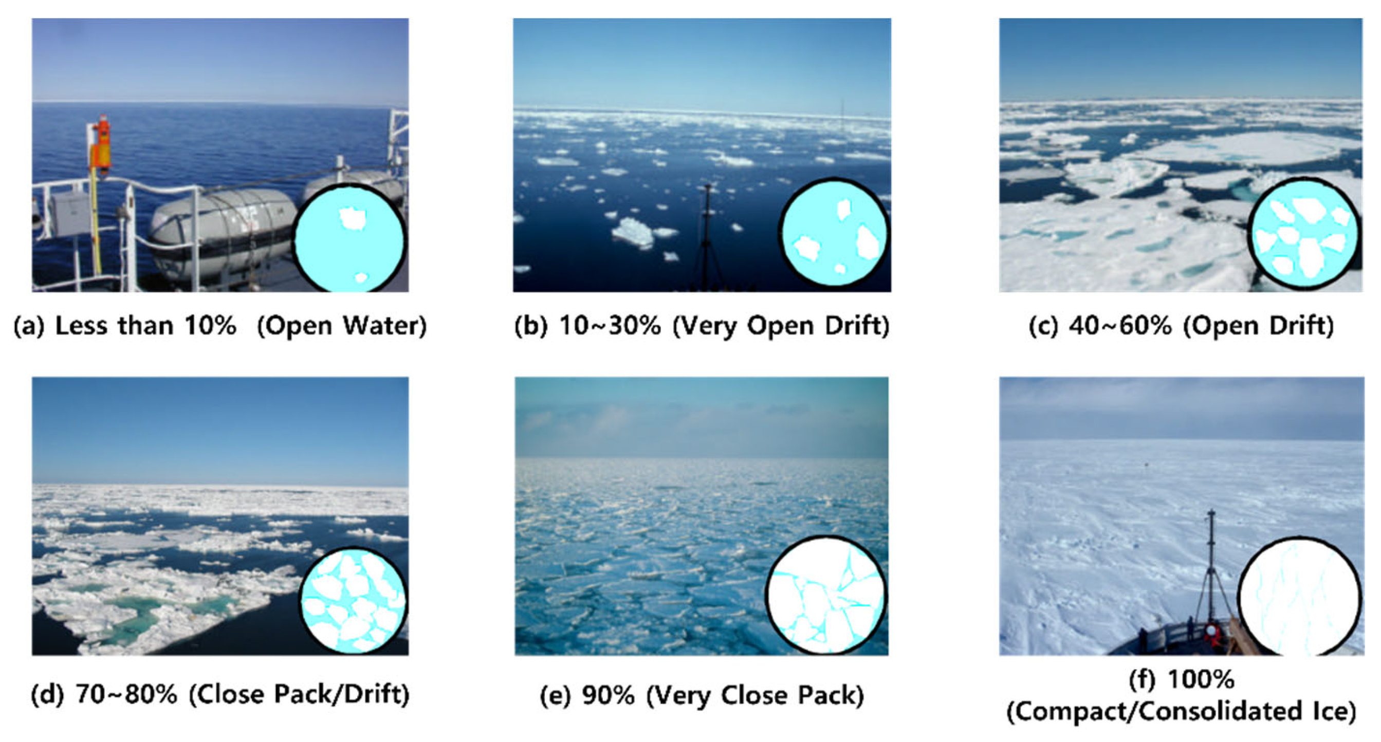
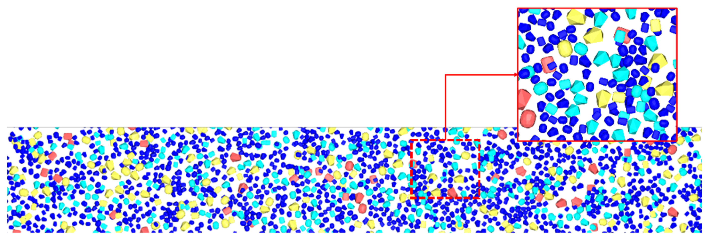
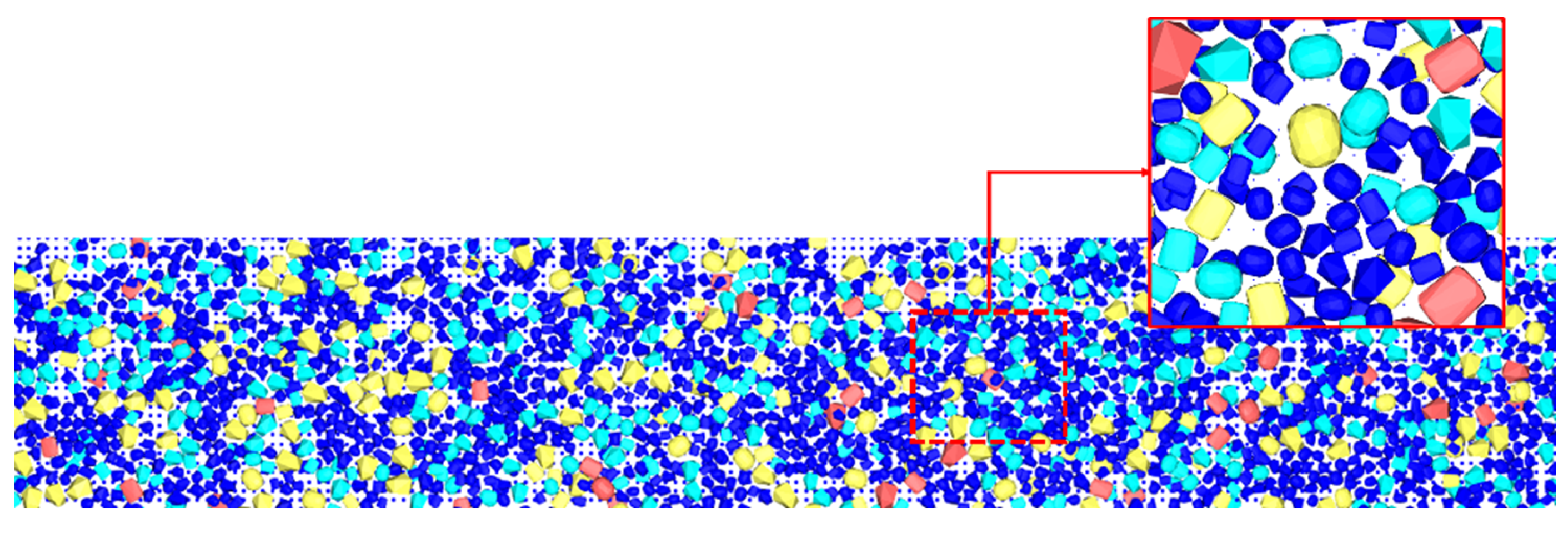
According to the Arctic Ice Regime Shipping System (AIRSS) [
47] developed by Transport Canada, one of the main factors defining the ice regime that affects ships operating in polar regions is ice concentration, which is defined according to the percentage of space occupied by ice in the route. In this study, ice concentrations of 60% and 80% were evaluated, as illustrated in
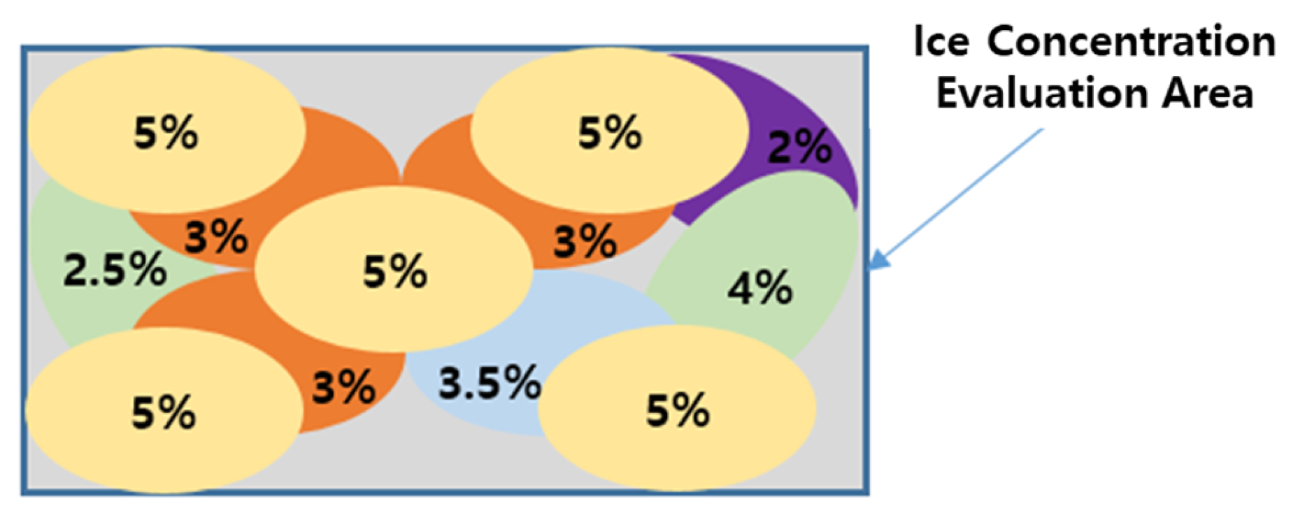
Figure 8. Ice concentration is defined as the ratio of the area occupied by an ice particle in the same two-dimensional view to the total area when viewed vertically in the area where the particle is located.
Figure 9 displays ellipsoid particles with a cross-sectional area comprising 5.0% of the total area, depicting the distribution of ice floe particles within the evaluated area for ice concentration. In the ice concentration calculation, the overlapping area between the floe particles is removed from the cross-sectional area. If a particle has an exposed cross-sectional area of 5.0%, but is partially covered by other particles, the exposed area is calculated by subtracting the overlapping area. In
Figure 9, there are five particles with an exposed cross-sectional area of 5.0%, one with 4.0%, one with 3.5%, three with 3.0%, one with 2.5%, and one with 2.0%, resulting in an ice concentration of 46.0%.
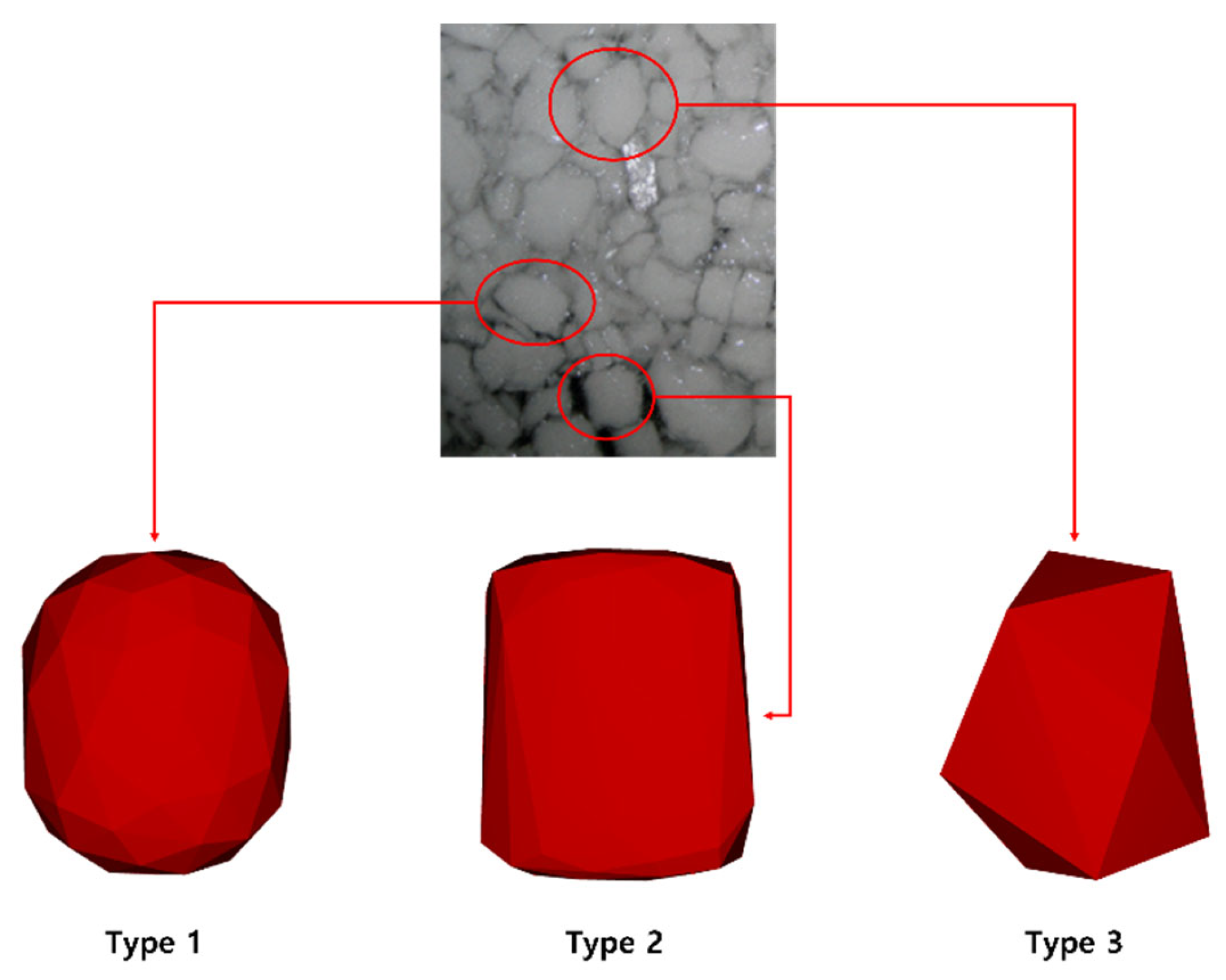
The shape of the ice particles was defined as described by Zhang et al. [
23]. The ice particle modeling results are shown in
Figure 10. The size distribution of the ice particles was determined by Liu and Ji [
22]: 25% of 1.0 m particles, 50% of particles larger than 1 m and smaller than 1.5 m, and 25% of particles larger than 1.5 m and smaller than 2.0 m. This size distribution was used for the three particle shapes. The sizes of the three different particle shapes were defined as the sizes of spherical particles with the same volume.
Figure 10 illustrates the ice particle shape modeling.
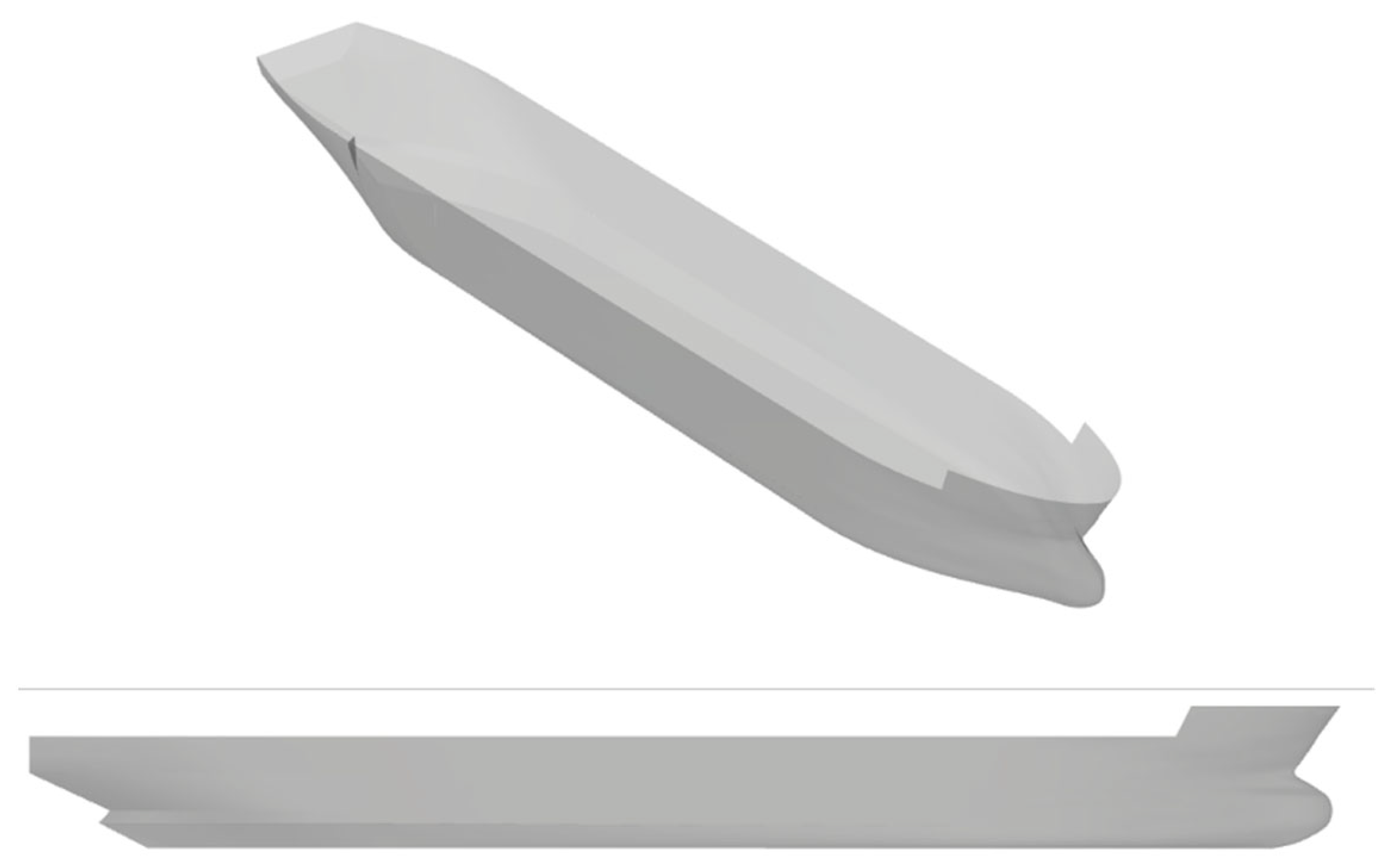
An oil tanker with a length of 43 m, a width of 6.5 m, a depth of 3.6 m, and a draft of 2.4 m was evaluated as shown in
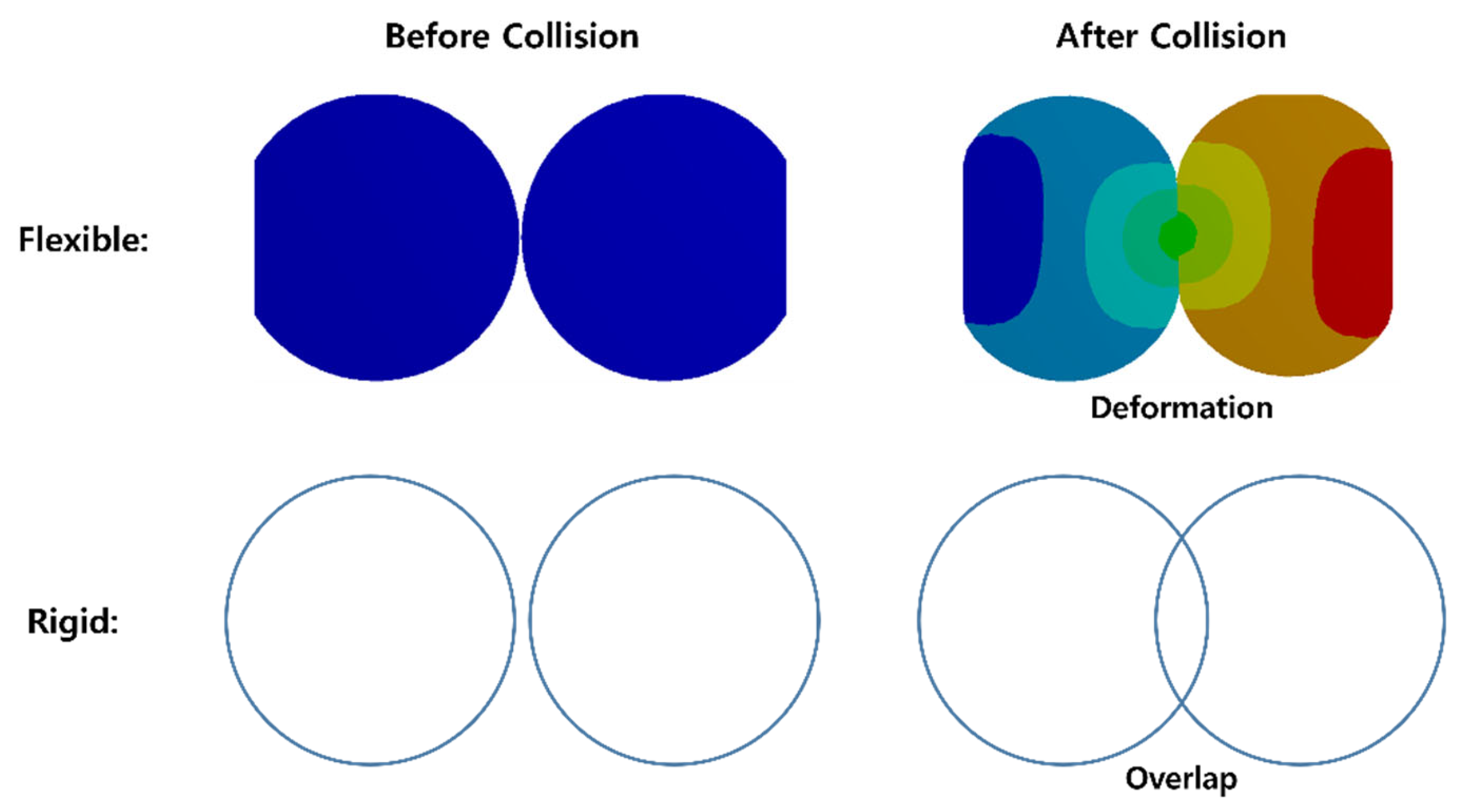
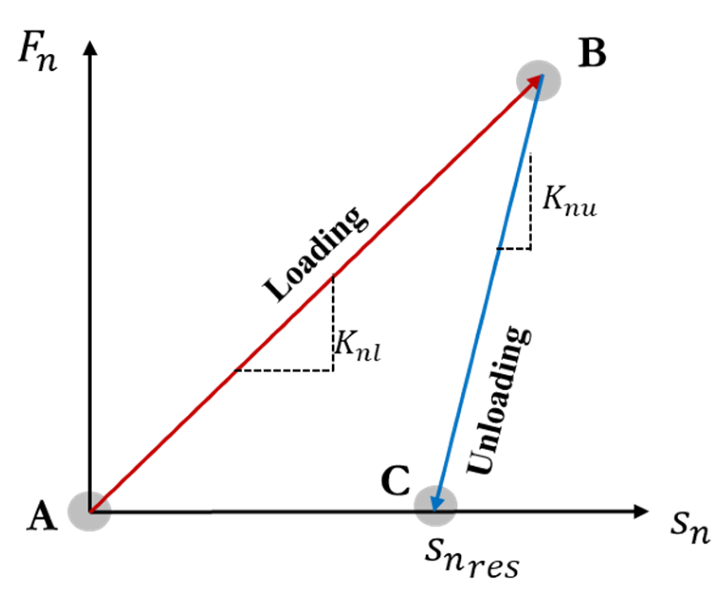
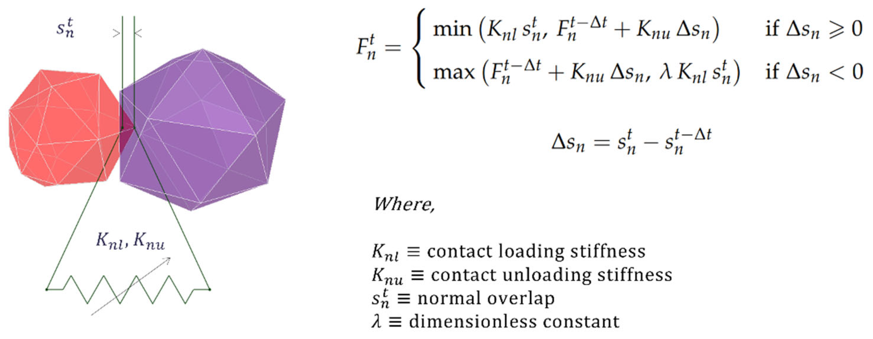
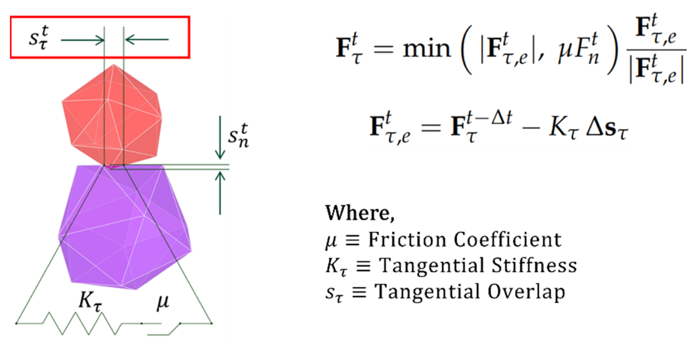
Figure 11. The HLS model used in this study calculates the normal contact force. In the evaluation of normal stiffness for a particle, the bulk Young’s modulus is employed as an alternative to the Young’s modulus (often referred to simply as elastic modulus). The bulk Young’s modulus is generally known to be approximately 1/50 to 1/100 of the value of the linear Young’s modulus. The LSCL model calculates the tangential force, and the normal stiffness of the HLS model affects the tangential stiffness. Therefore, the material properties of ice can be defined differently from the well-known material properties of floes. In this study, the material properties are defined by referring to the results presented by Lee [
48]. In order to ensure the reliability of the material properties required for the numerical model, Lee [
48] performed the analysis under the same conditions as the experiments performed in the previous study. The properties were defined in such a way that the difference between the experimental and analytical results could be minimized. Lee [
48] validated the reliability of the bulk Young’s modulus by analytically replicating the experiments originally conducted by Do and Kim [
49]. In these experiments, cubic ice blocks were compressed in a laboratory setting to assess the relationship between applied force and compressive displacement. The analytical results from Lee [
48] were found to be consistent with these experimental findings. It is important to note, however, that data obtained from any single experiment cannot fully capture the material properties of all ice types. Consequently, there exists an inherent challenge in needing to compare both experimental and analytical results each time to determine the material properties most suitable for specific evaluation conditions. Kietzig et al. [
26] present a friction coefficient of 0.13 for a hull that has been in service for many years. In order to define the tangential stiffness that has the same effect as the friction coefficient of 0.13, Lee [
48] conducted an analysis in which the ice cube was compressed and then slid. Furthermore, the parameters for ice density and Poisson’s ratio in this study were defined in reference to the findings of Kim et al. [
9]. Through a series of repeated experiments, Kim et al. [
9] reported a Poisson’s ratio of 0.003 for ice. Additionally, van den Berg [
11] reported values below 0.003, which are in alignment with the parameters used in the present study. The material properties applied to the analysis are shown in
Table 2 and
Table 3.
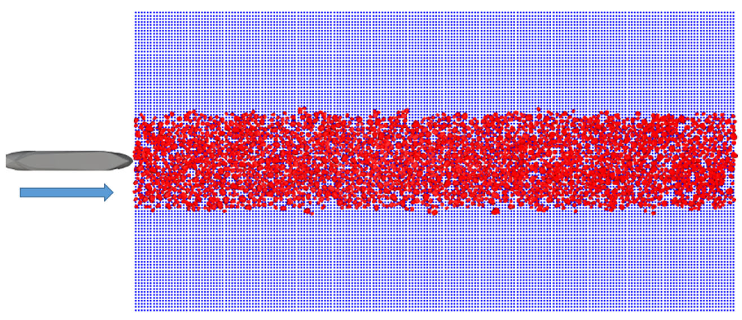
The DEM analysis conditions reflecting the above conditions are shown in
Figure 12. The evaluation models were constructed by initially placing particles according to the ice concentration on the surface of the 200 m route and then moving the hull. The blue area in
Figure 12 is the seawater area defined by the CFD analysis result. To perform the evaluation in the same ice arrangement for each ice concentration, the particle arrangement was stored and used as an initial condition for each evaluation case. The initial arrangements of drift ice according to ice concentration are shown in
Figure 13 and
Figure 14.
4.2. Coating Material Wear Assessment
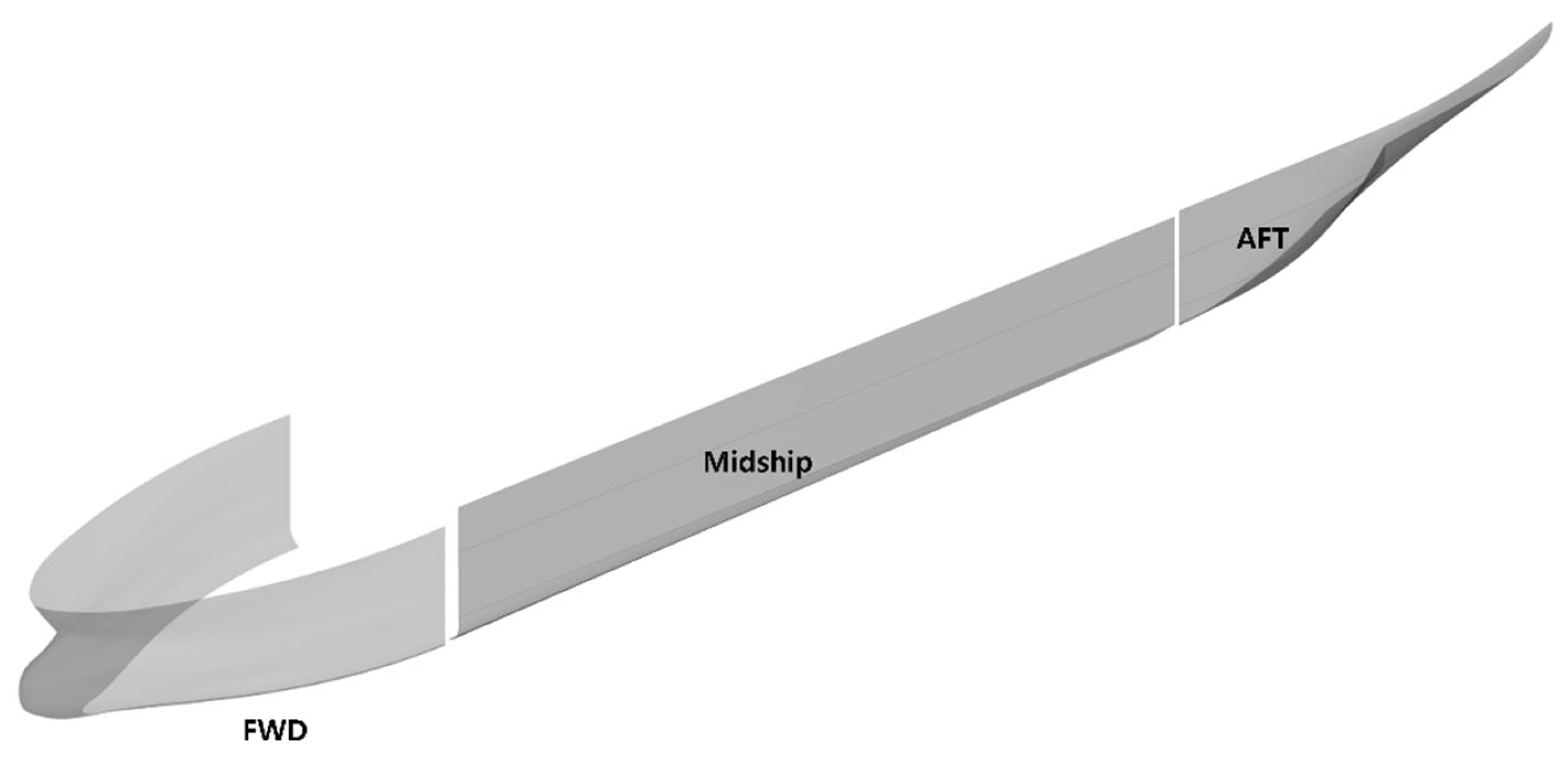
The evaluations were performed assuming a scenario in which a coating material such as paint was separated from the hull by friction between the ice and the hull. Evaluations were performed at ice concentration of 60% and 80% and ship speeds of 4, 6, and 10 knots.
Given that the coating material is very thin compared to the thickness of the hull, the effect of material loss on the flow and behavior of ice is negligible. Therefore, the analysis was performed without reflecting the shape change, and the wear was evaluated based on the shear work according to Archard’s wear law. Given that wear is a type of damage that occurs over a long period, it was not evaluated as a result of a specific point in time but was evaluated as an accumulated value on the hull after passing a 200 m route. Shear work, tangential force, and sliding distance were evaluated in the form of cumulative values for each evaluation condition according to the Archard wear law. The hull was divided into three regions to conduct the evaluations: forward (FWD; i.e., the bow), midship, and after (AFT; i.e., the stern) of port as shown in
Figure 15.
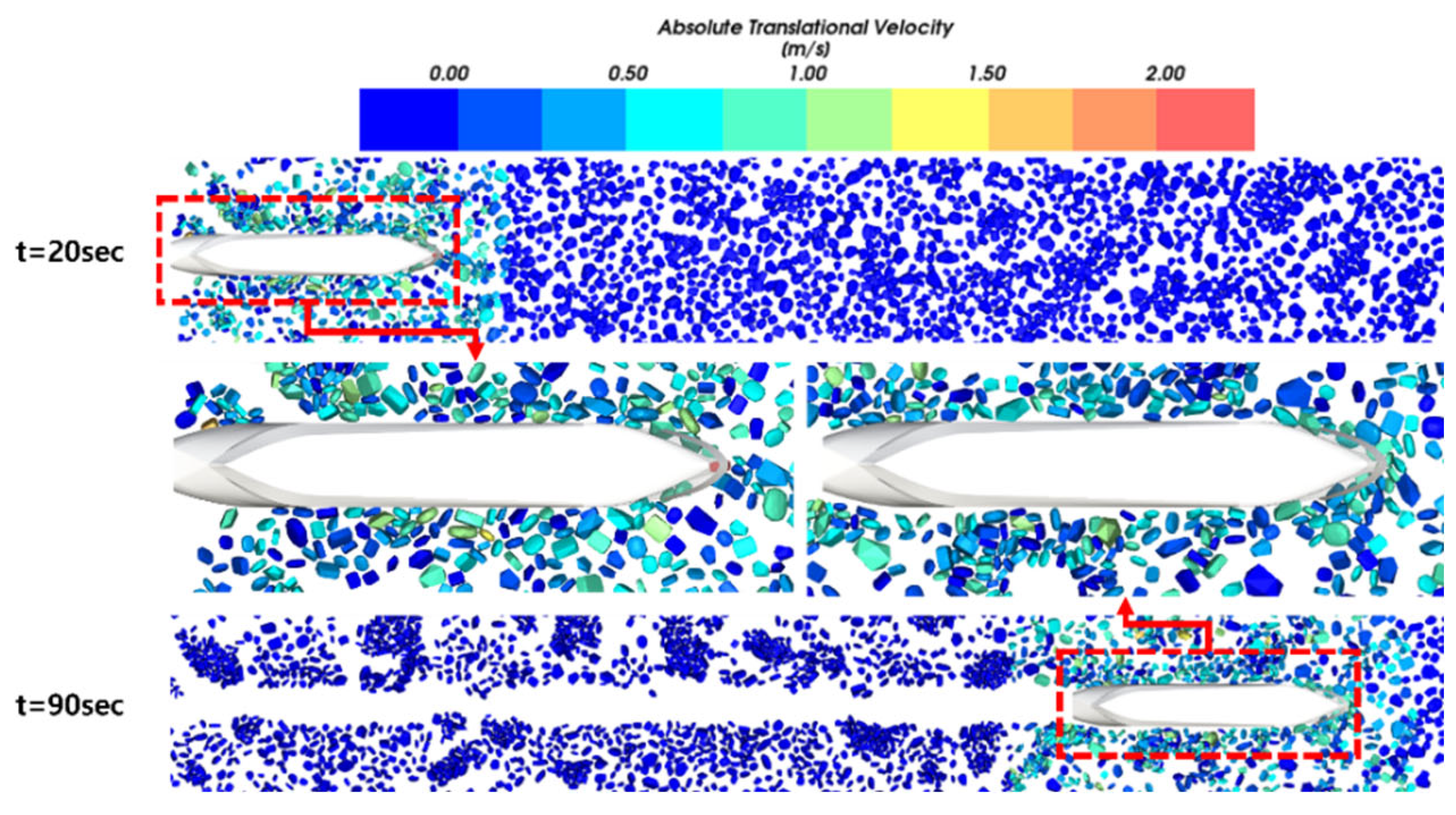
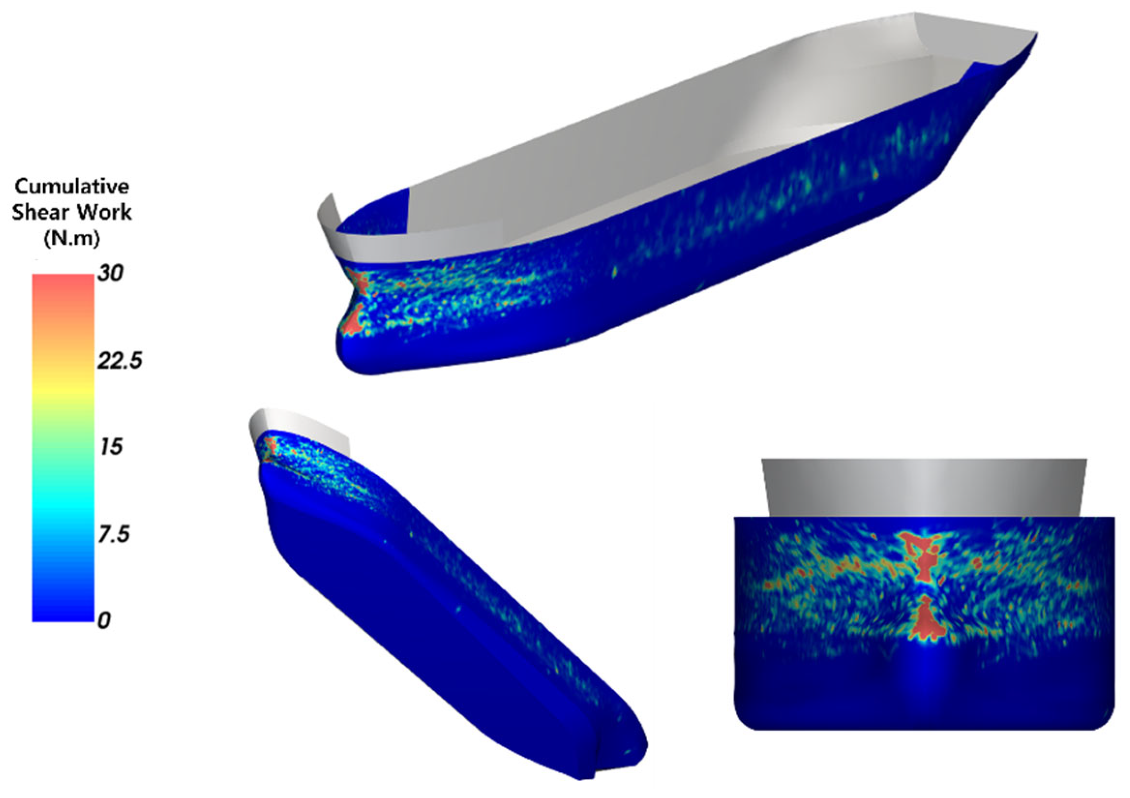
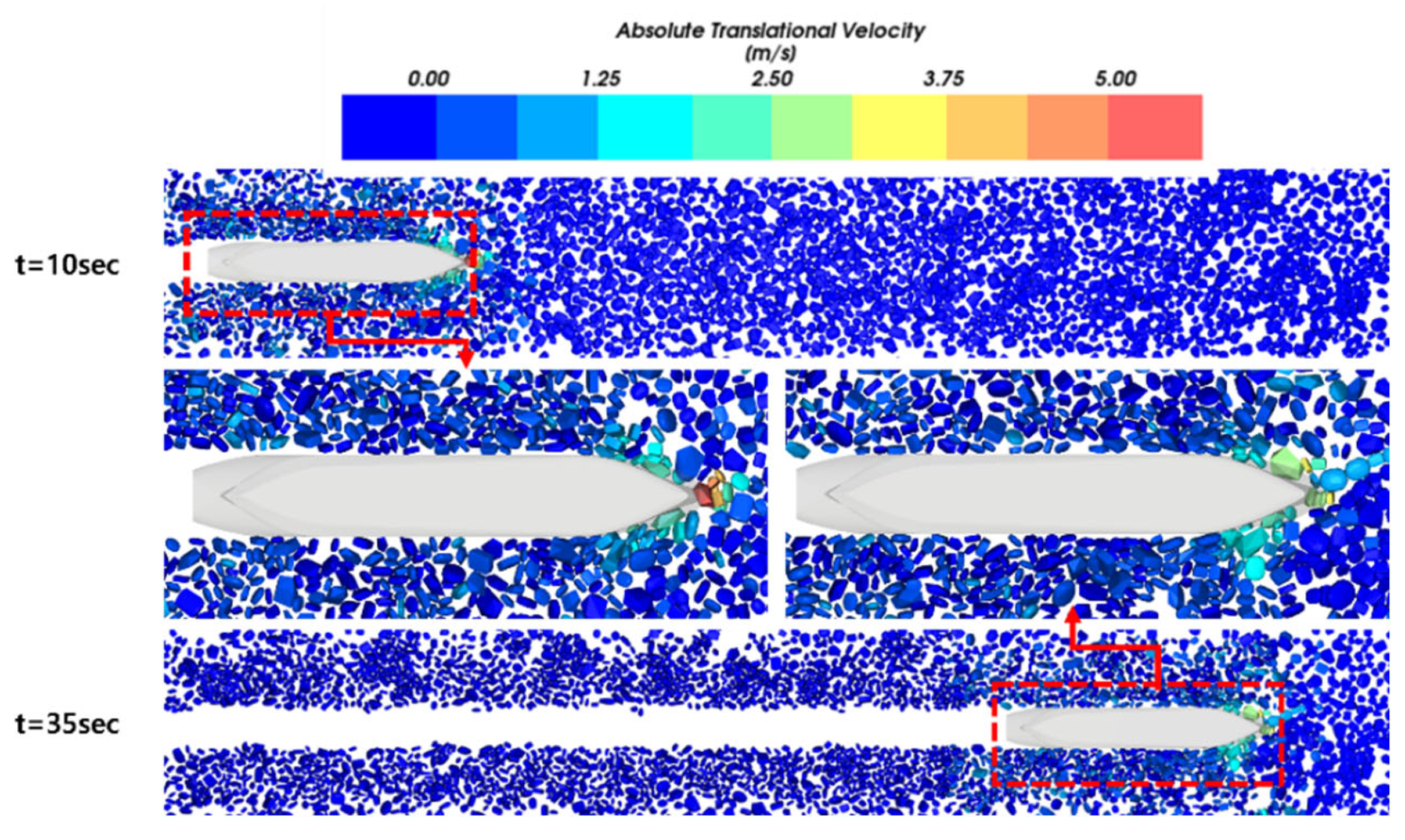
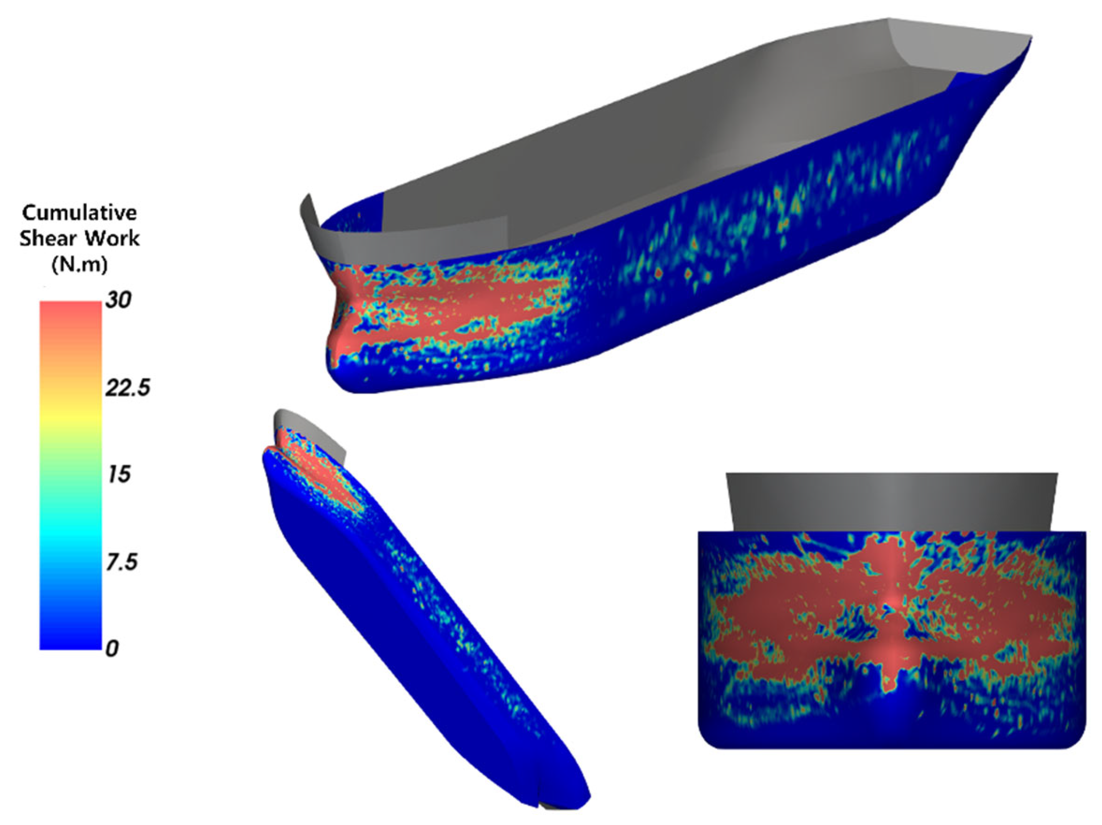
Six analysis scenarios were simulated by combining three cases of ship speed and two cases of ice concentration. Among the six simulated scenarios,
Figure 16 and
Figure 17 show the simulation results of the scenario with the slowest ship speed and the lowest ice concentration (4 knots, 60%), whereas
Figure 18 and
Figure 19 illustrate the scenario with the fastest ship speed and the highest ice concentration (10 knots, 80%).
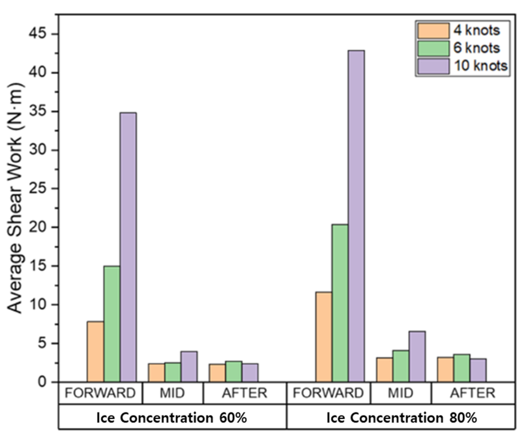
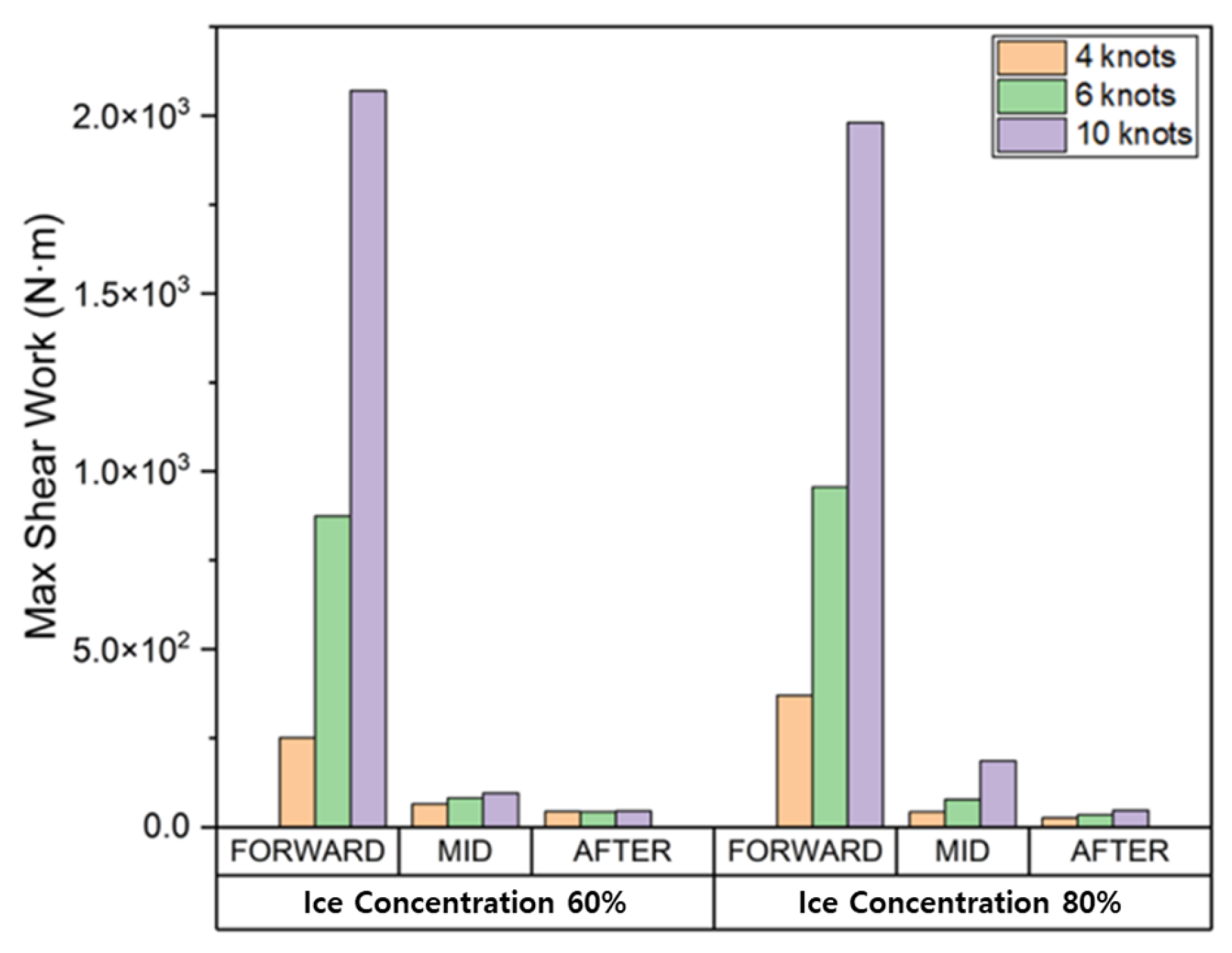
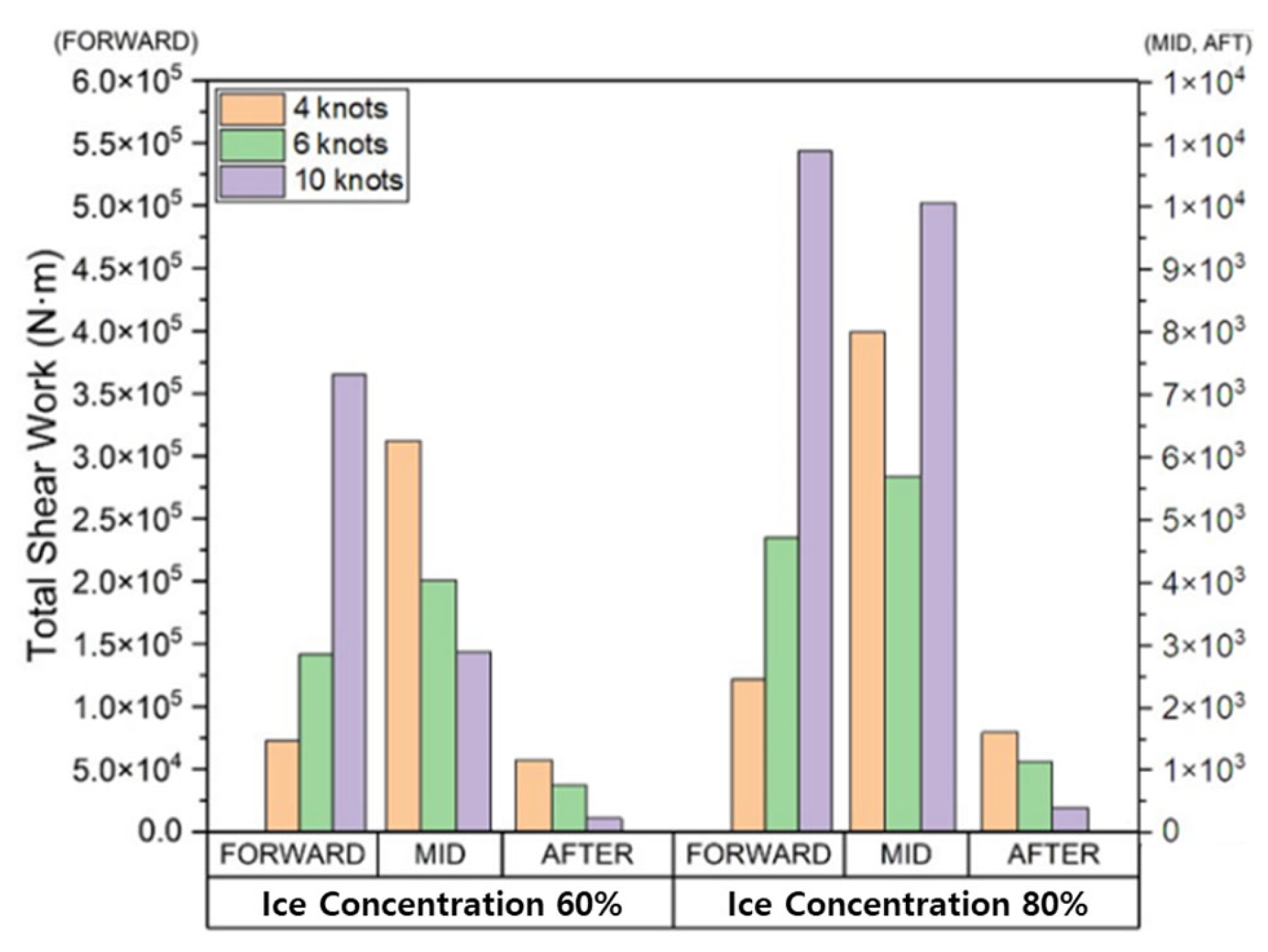
The average, maximum, and total cumulative shear work causing wear on the FWD, midship, and AFT are shown in
Figure 20,
Figure 21 and
Figure 22.
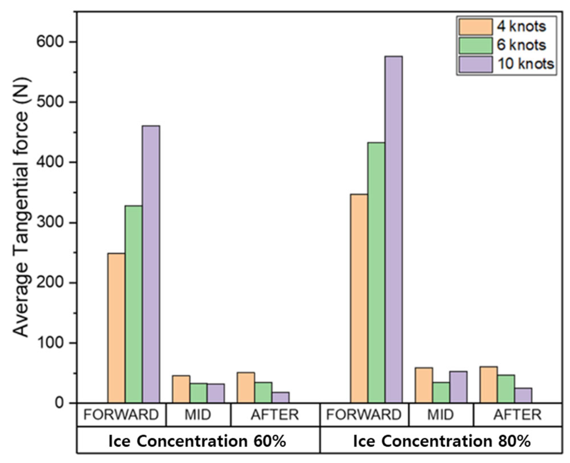
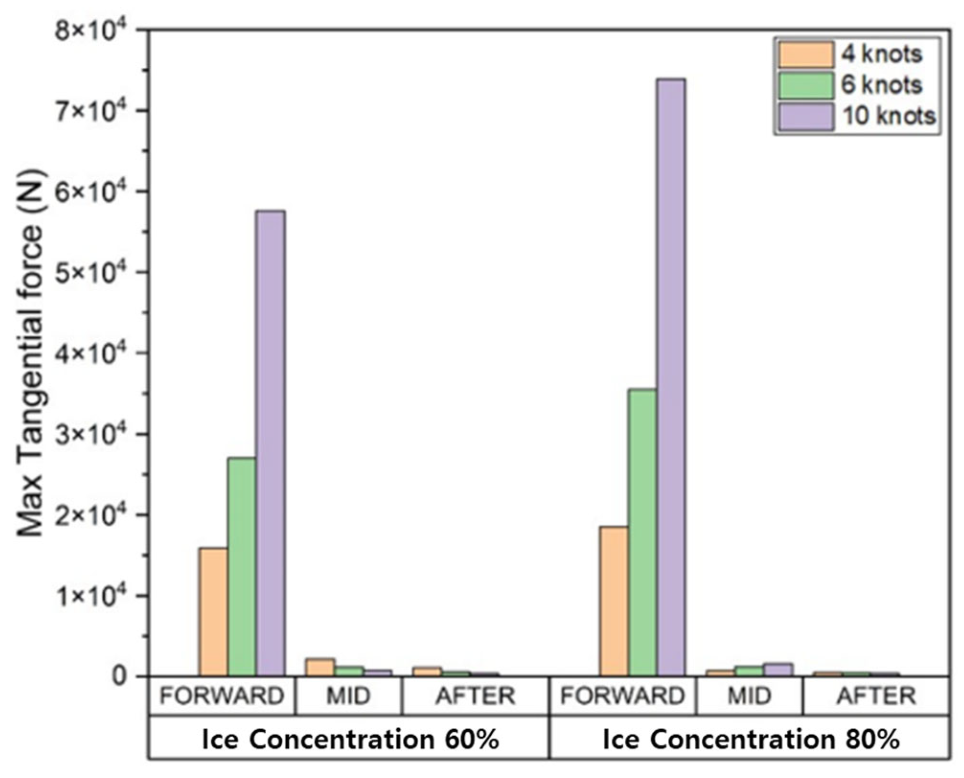
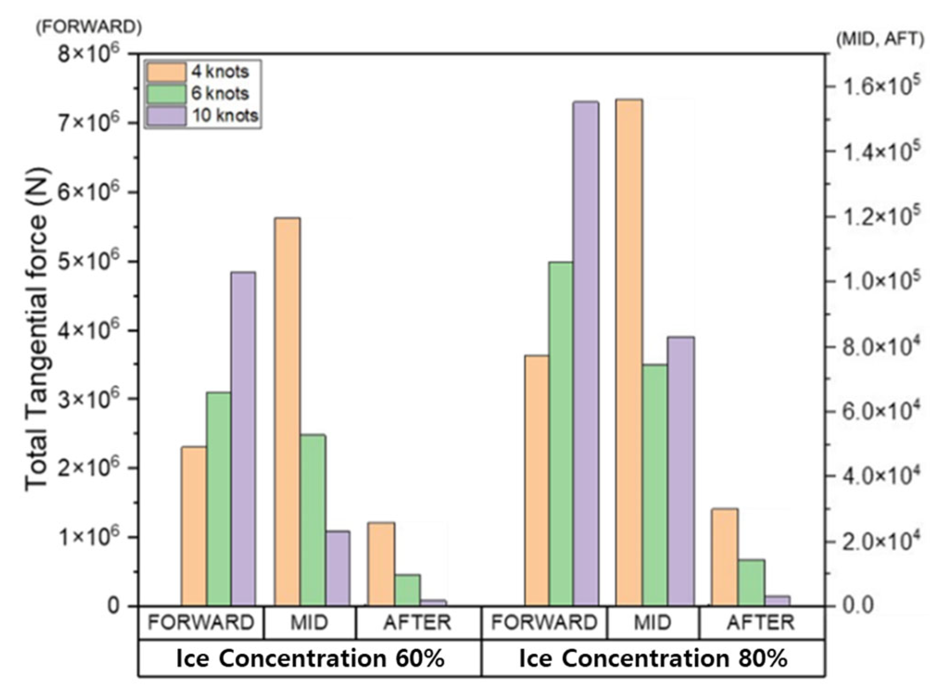
The average, maximum, and total cumulative tangential force, which are components of shear work, at the FWD, midship, and AFT are shown in
Figure 23,
Figure 24 and
Figure 25.
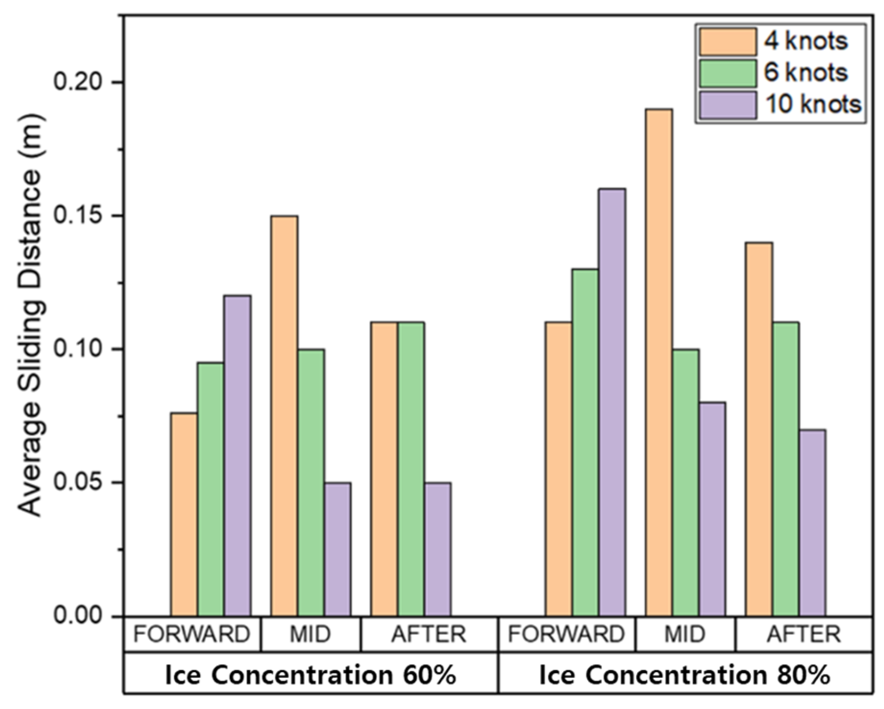
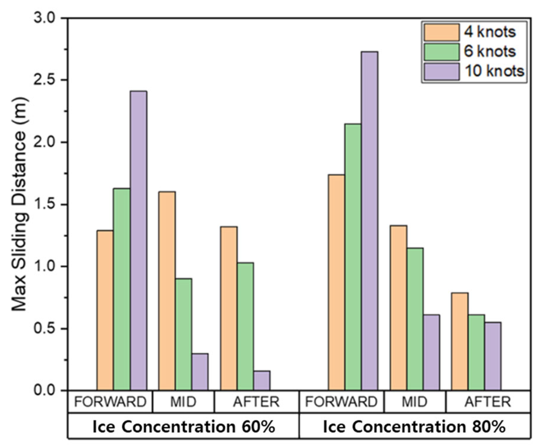
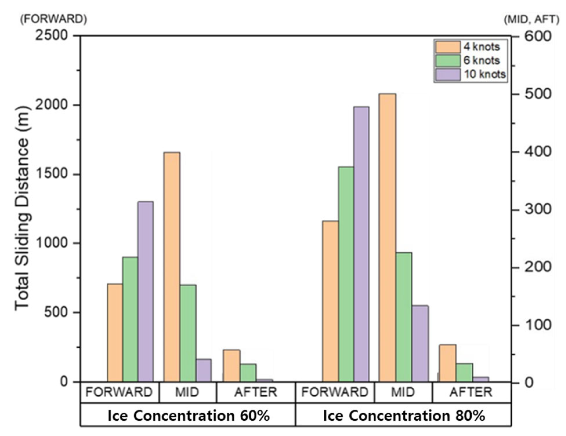
The average, maximum, and total cumulative sliding distance, which are components of shear work, at the FWD, midship, and AFT are shown in
Figure 26,
Figure 27 and
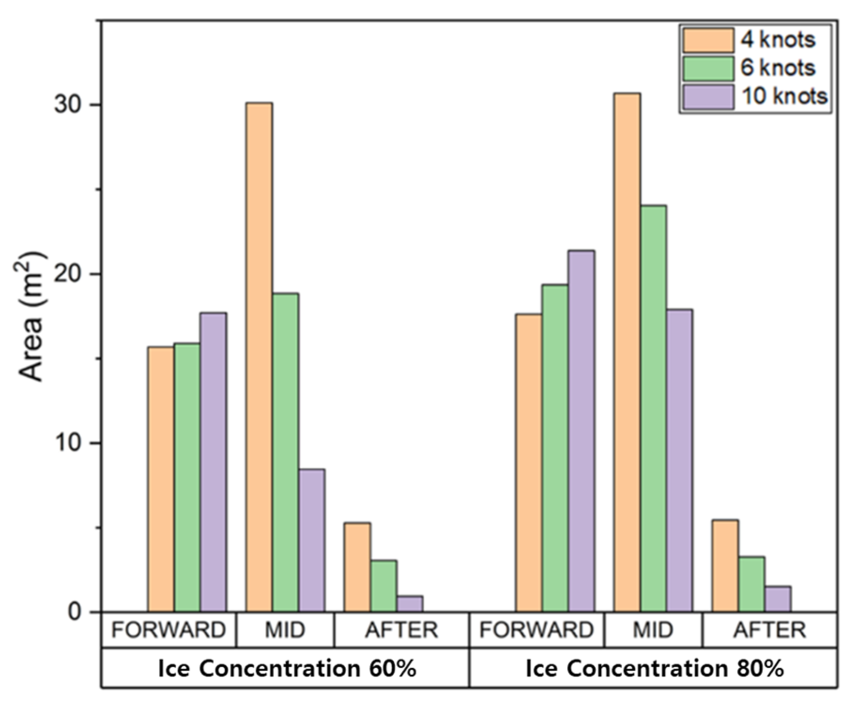
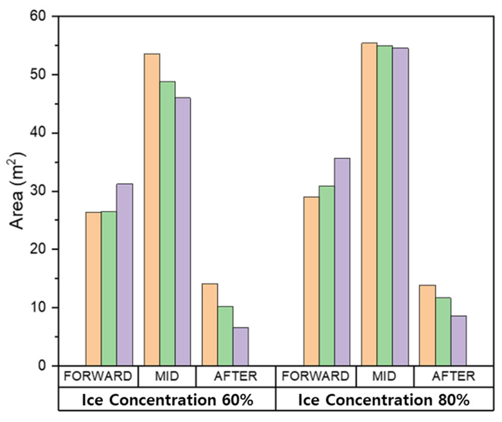
Figure 28. The total area affected by wear is shown in
Figure 29.
Our findings indicated that the accumulated total shear work, tangential force, and sliding distance in all areas at 80% ice concentration was greater than 60%. As the ice concentration increases, the cumulative results of each item increase because the number of collisions also increases.
Our results also demonstrated that as the ship speed increases, the cumulative shear work, tangential force, sliding distance of the drift ice per unit time, and wear affected area at the FWD also increased. These results indicate that the wear occurs in a deep and wide area as the ship speed and the ice concentration increases. Since the direct collision between drift ice and the hull is dominant in the FWD, the tangential force and sliding distance generated in each collision increases as the ship speed increases. Therefore, the cumulative average, maximum, and total amounts of each evaluation item tended to increase.
In the midship and AFT, as the ship speed increases, the cumulative shear work, tangential force, sliding distance, and the area affected by wear tend to decrease inversely. This is because the drift ice, which first collided with FWD, rubs against the hull while flowing along the outer wall. When the ship speed is relatively slow, the drift ice that first collided with FWD moves smoothly along the outer wall of the hull. However, as the ship speed increases, it tends to move away from the hull rather than flowing along the outer wall.
This trend is clearly shown in
Table 4, which summarizes the total cumulative shear work per unit area as a ratio of FWD. Given that the total volume of wear according to Archard’s wear law is proportional to the shear work, the results are summarized based on the shear work. The total shear work accumulated per unit area of the midship and AFT relative to the FWD region was evaluated to be as high as 4.99%, and the ratio tended to decrease as the speed increases. As expected, our results demonstrated that FWD directly collides with the drift ice, and therefore the amount of wear and the ship speed are directly related. In contrast, midship and AFT wear was not related to ship speed because the particles that first collided with the FWD-induced wear while moving along the outer wall of the hull. Therefore, to prevent abrasion in the FWD, the ship speed must be reduced, or sufficient reinforcement must be provided according to the ship speed. Moreover, to prevent midship and AFT wear, the outer shape of the hull could be redesigned to minimize the damage caused by the drift ice that first collides with the FWD.
Models without shape changes due to wear-induced material loss can also evaluate the wear depth by applying the accumulated shear work to the Archard wear law. As shown in Equation (27), the wear depth was evaluated by multiplying the accumulated shear work by the volume loss ratio C according to the Archard wear law. The wear depth was evaluated by dividing the evaluated wear volume by the individual cell area of the hull surface. The volume loss ratio C per unit shear work was defined as 5 × 10
−7m
3/J, which is the same as the value applied in the following section. The wear depth according to ship speed and ice concentration for each hull position was evaluated as shown in
Table 5. Considering the distance traveled by the ship, the predicted wear is very large. By adjusting the parameters of the Archard law, smaller wear values that align more closely with expectations can be achieved. However, the primary focus of the present study was to propose a numerical model capable of predicting the wear resulting from ice collisions. Therefore, the development of the numerical model was our priority rather than the achievement of accurate wear predictions.
4.3. Hull Material Wear Assessment
In this section, the simulations were conducted assuming that the material of the hull is lost due to the accumulation of friction with the drift ice. The evaluations were performed at ice concentrations of 60% and 80% and ship speeds of 4, 6, and 10 knots. Wear-induced material loss leads to changes in the hull shape. In turn, these deformations can affect the flow of drift ice. To account for these dynamic changes, the analyses were performed by updating the shape change in real time, and the amount of material loss due to shear work was evaluated according to the Archard wear law. In Equation (25), C, which represents the volume lost per unit of shear work, was defined as
m
3/J, and the shape deformed by wear was automatically updated every 0.005 s. That is, the shape change due to abrasive wear was added in the analysis conditions described in
Section 4.1.
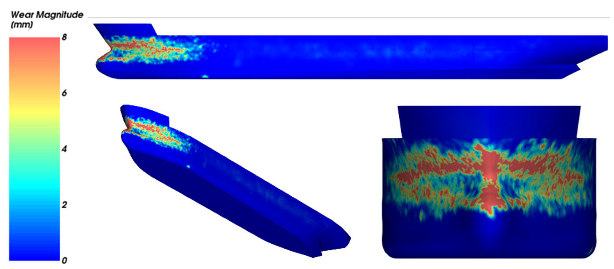
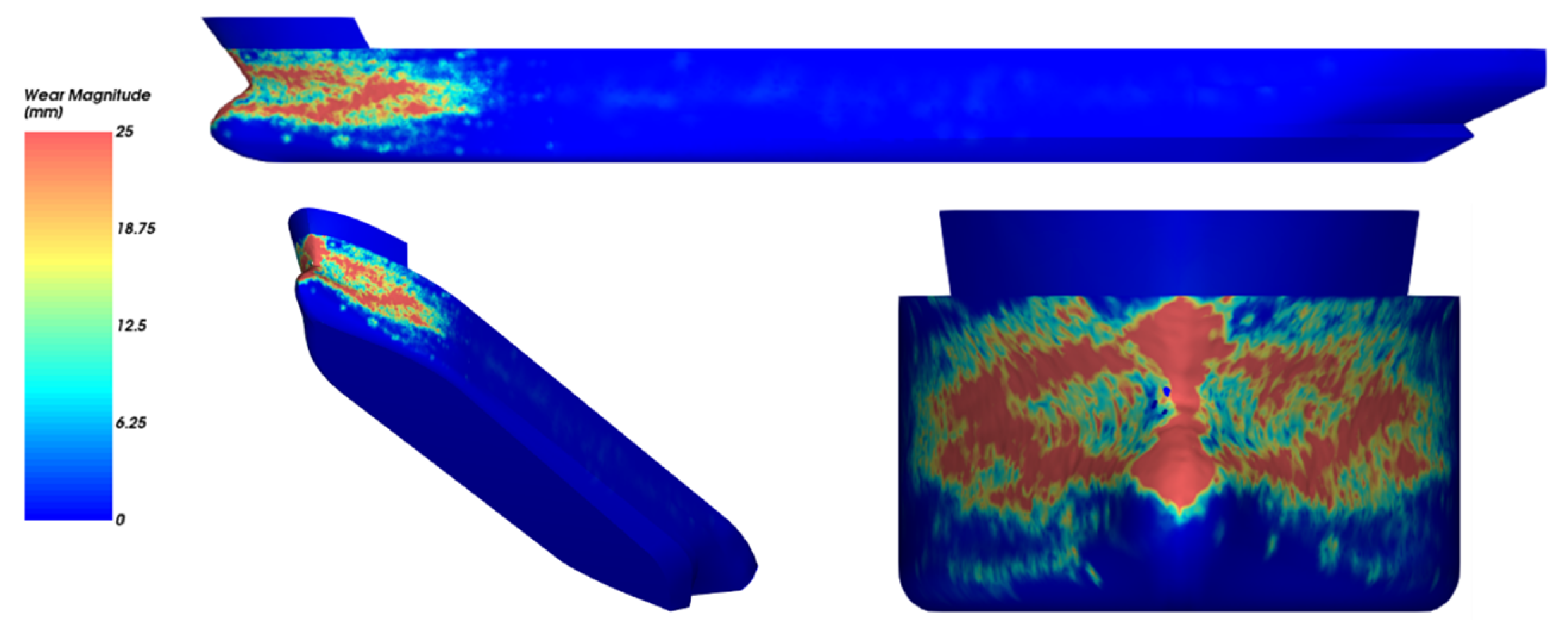
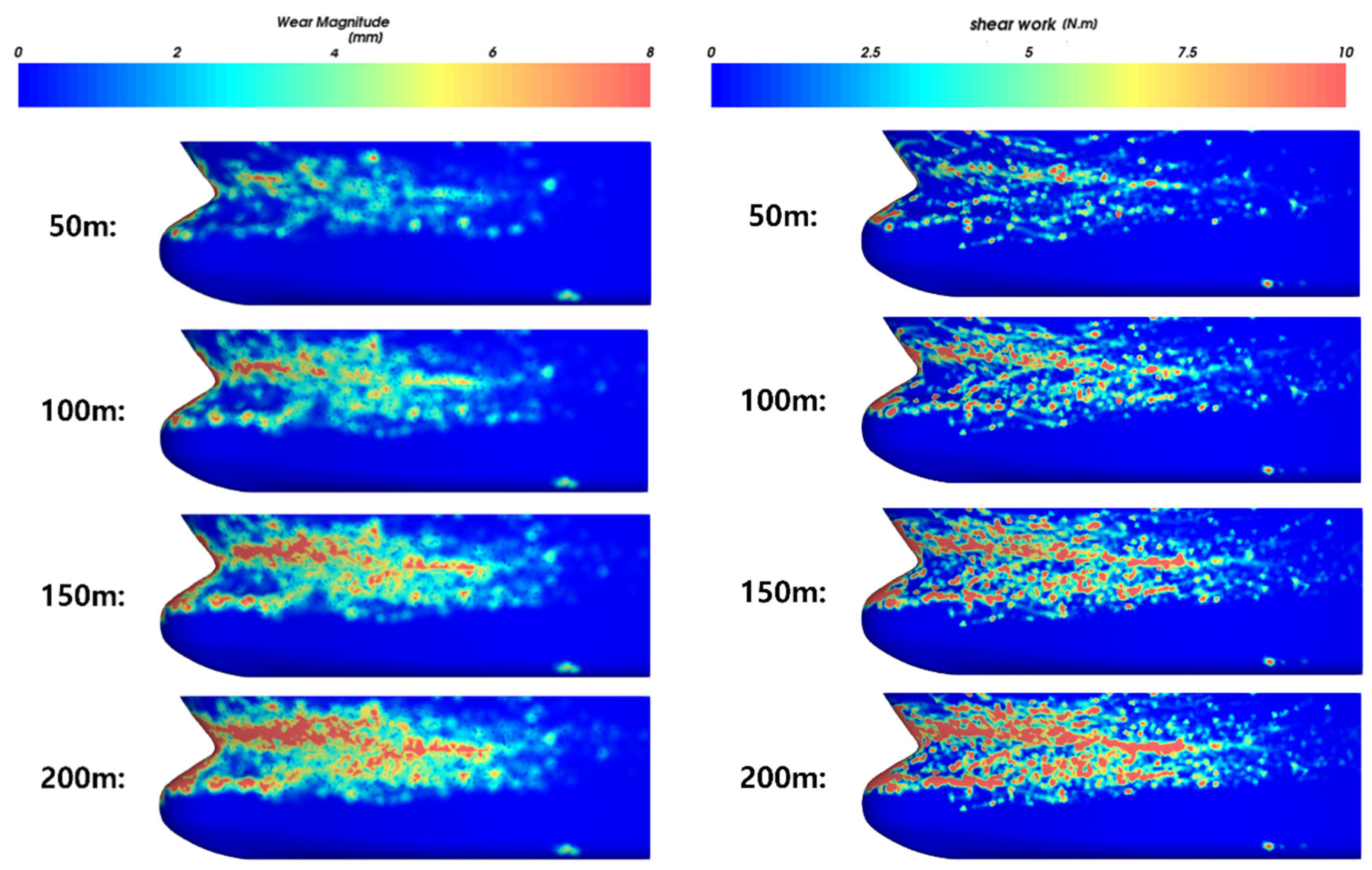
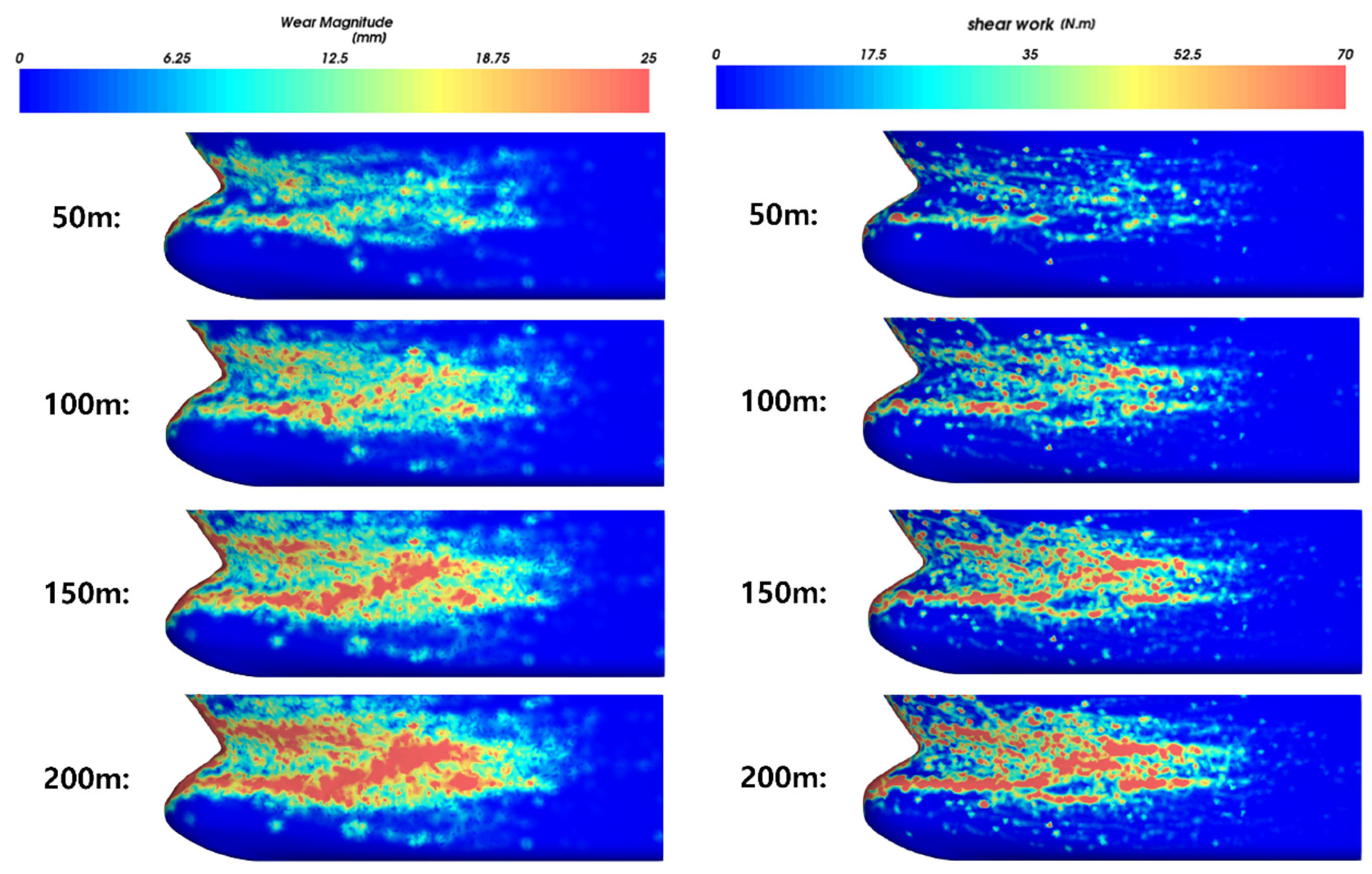
Among the six simulation scenarios, the analysis results of the scenario with the slowest ship speed and the lowest ice concentration (4 knots, 60%) and the scenario with the fastest ship speed and the highest ice concentration (10 knots, 80%) are shown in
Figure 30 and
Figure 31, respectively.
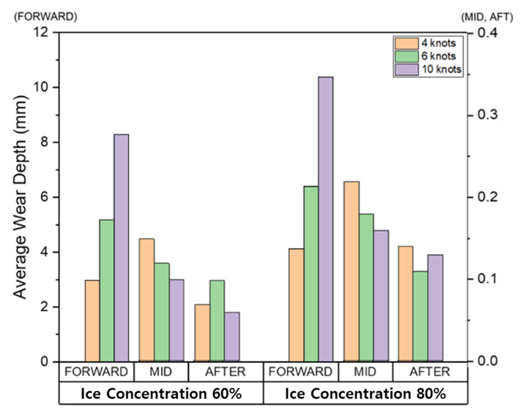
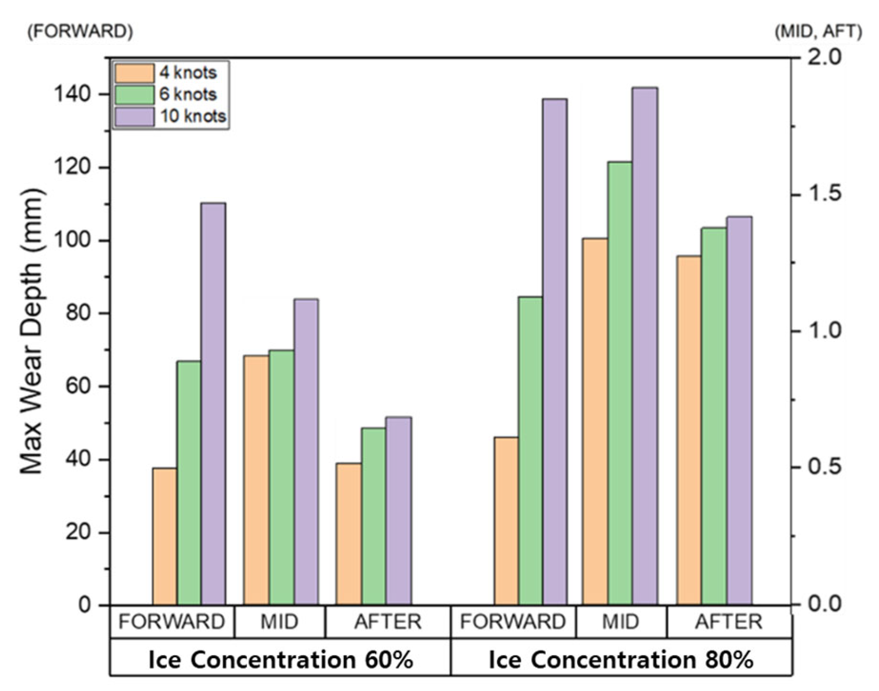
For each evaluation condition, the average, maximum wear depth, and total area affected by wear in the FWD, midship, and AFT are shown in
Figure 32,
Figure 33 and
Figure 34.
In the evaluation model considering material loss due to wear, as the ice concentration increases, the frequency of collisions with drift ice increases, and therefore the amount of wear tends to increase. The effect of ship speed tends to be different for each area. In the FWD area, as the speed of the ship increases, the average and maximum wear depth increases, and the area affected by wear also widens. In other words, the ice particles wear the hull more deeply and over a wider area. In the case of the midship, as the ship speed increases, the average wear depth and area tend to decrease, and the maximum wear depth tends to increase. If the ship speed is slow, a relatively large area is worn because the particles that first collide with the FWD move smoothly and accumulate along the outer wall of the hull. At the point where the shape of the vessel changes from the curved surface of the FWD to the straight walls of the midship, the maximum wear depth tends to increase as the ship speed increases because the drift ice that first collided with the FWD surface moves along the hull and is repeatedly separated. Similarly, since the same behavior appears at the point where the shape changes from the straight midship to the curved AFT region, our findings confirmed that the wear depth increased as the ship speed increased.
In order to accurately assess hull wear through a numerical model, several challenges remain. The first is to accurately simulate the behavior of the flow and floe in the channel. To ensure the accuracy of the analysis of each phase of the flow and particles, we used solvers specialized for each phase. We also applied one-way coupling, which is known as a method that can achieve both accuracy and efficiency of the analysis based on previous studies. The second is the reliability of the material properties that affect the behavior of the material and the magnitude of the impact load. Reliable material properties, defined through comparison of experimental and analytical results, were incorporated into the numerical model. The final step is the definition of material properties that can determine the amount of wear. In this study, the wear amount was evaluated by applying the Archard wear law, where the wear amount is determined by the shear work and the material constant C, as shown in Equation (25). If the floe and surrounding flow can be accurately evaluated, and the load can be accurately evaluated, the shear work will be accurately evaluated. If there are enough data to verify the reliability of defining C, the evaluated wear amount will also be accurate, but we recognize that this is a limitation of this study. In order to validate the numerical model, the values of material properties related to wear must first be measured through experiments, and the wear history must be measured in the actual ship’s operating environment (speed, ice distribution, and concentration) and on the ship’s surface. Unfortunately, such measurement work is very large and beyond the scope of this study, so the data required for validation were not available. Defining a reliable C remains a challenge and should be the subject of further research.
The core objective of our study was to propose a numerical model capable of predicting hull wear resulting from ice collisions, with a specific focus on the simulation methodology and considerations related to wear estimation. In order to clarify the effect of changes in hull shape change due to wear, the C was intentionally defined as an excessively large value.
4.4. Comparison of the Results According to the Evaluation Method
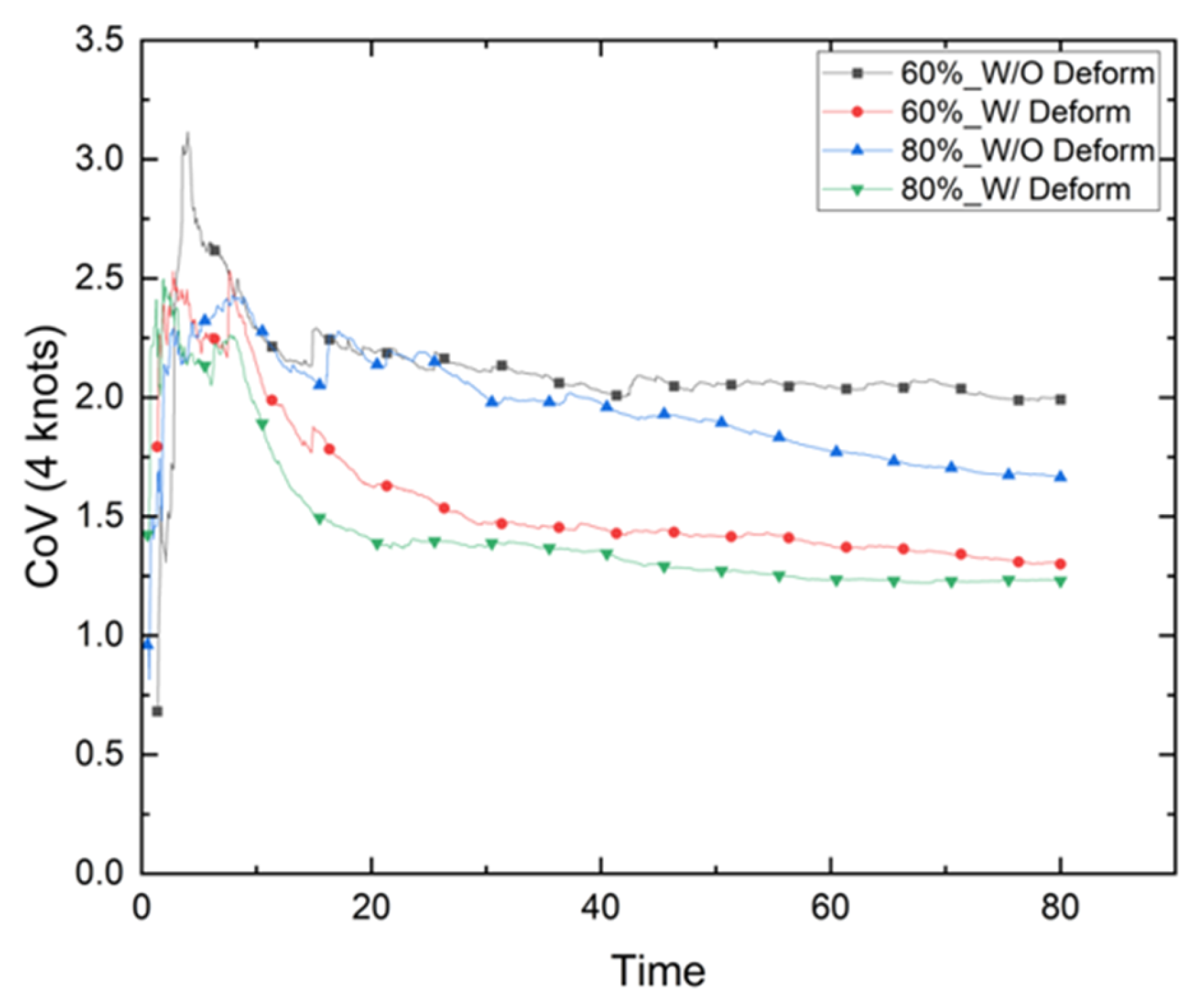
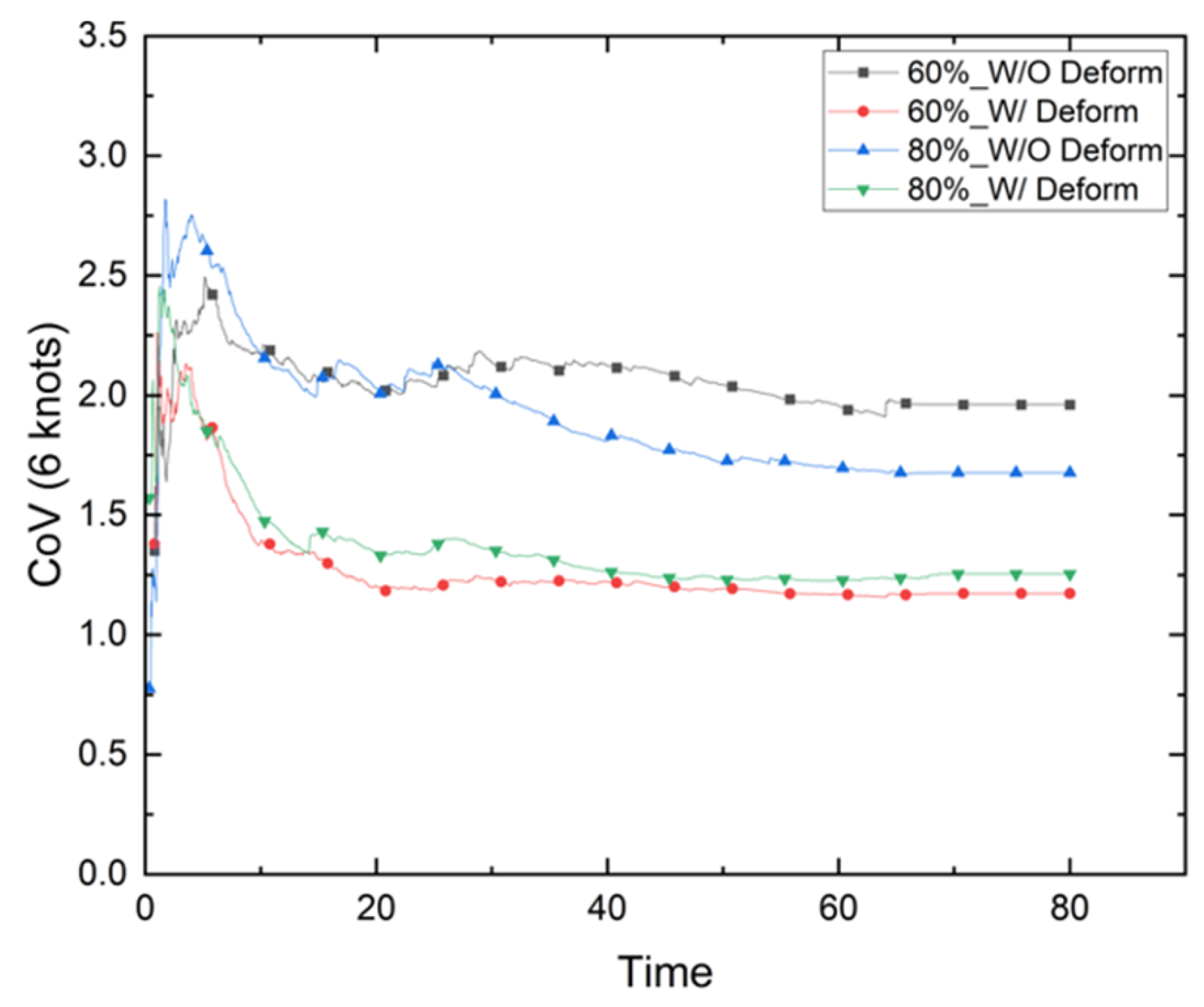
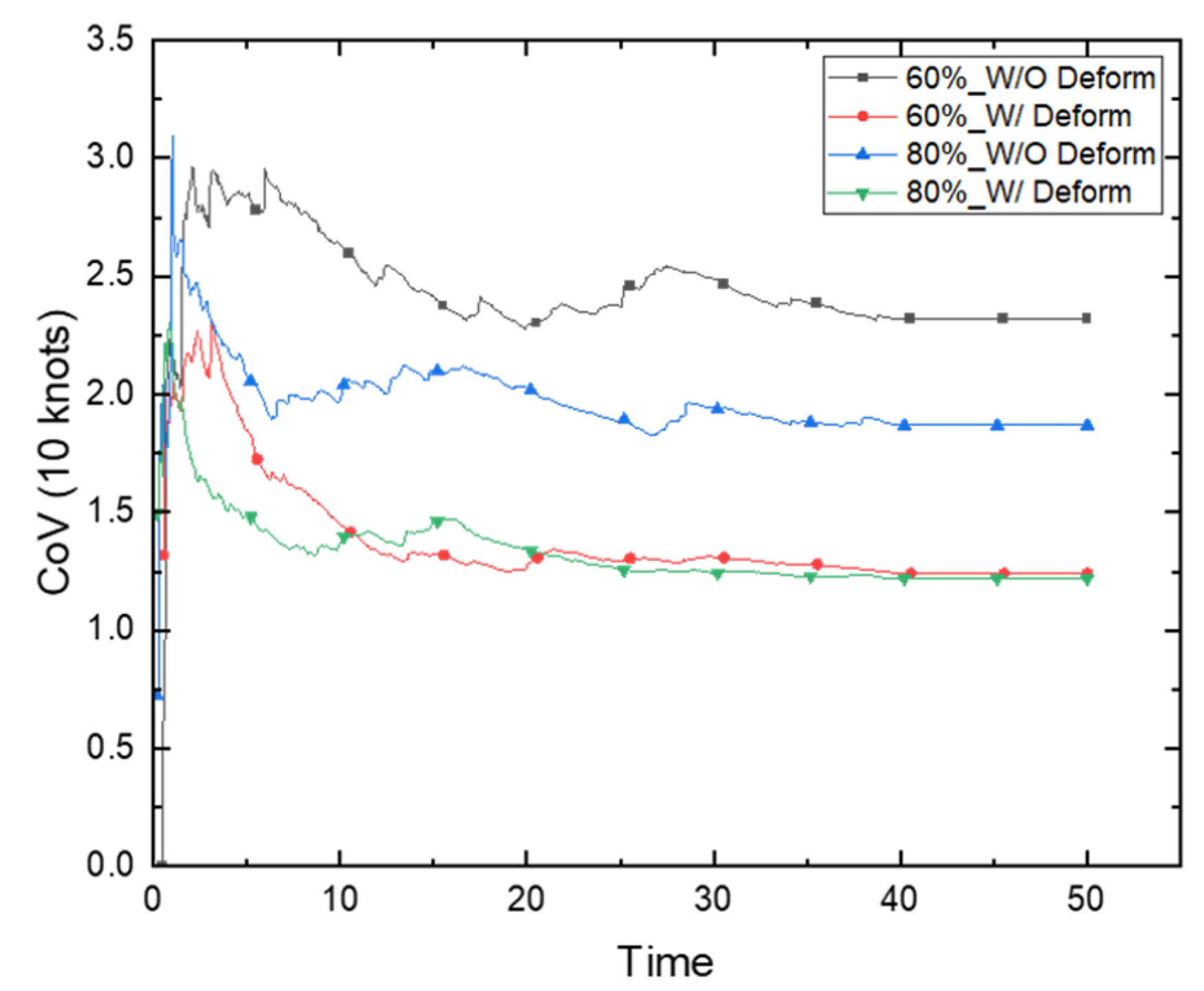
Two evaluation models were examined in this study according to two different phases of hull wear. The first was the painting surface wear that may occur in the early stages of the operation, and the second was the loss of hull material due to the accumulation of friction with drift ice with extended operation periods. In terms of numerical analysis, the first method was used to evaluate wear based on shear work without considering the change in hull shape due to wear, whereas the second method was used to evaluate wear by accounting for the effect of wear-induced shape changes of the hull on the dynamics of the ice particles. Our results confirmed that the wear of the FWD area was significantly greater than that of the midship and AFT. The characteristics according to the evaluation method were analyzed based on the results of the FWD area. In the case of the model that accounted for hull deformation, the results cannot be compared with the same value as the model without hull deformation because the mesh constituting the hull model is continuously deformed. Therefore, our study compared the amount of hull deformation due to wear in the model with hull deformation and the shear work that causes wear in the model without hull deformation. To compare the wear patterns for each numerical model, the evaluation results of the two analysis methods were compared. The coefficient of variation (CoV) was used to compare wear patterns with different physical indices. The CoV is an index that is commonly used to compare two sample groups with a large difference in mean values or to compare data with different units. It is defined as the ratio of the standard deviation to the mean.
The analysis results were compared in the scenario with low ice concentration (4 knots, 60%) and the scenario with the fastest line speed and the highest ice concentration (10 knots, 80%).
Figure 35 and
Figure 36 illustrate the wear shape and shear work for each numerical model. Since the structural boundary conditions do not change from the perspective of the drift ice in the model that does not consider the shape change, the area where most of the shear work occurs in the early stage did not change substantially and it continuously received a large load. Therefore, a band shape tended to form because the shear work was concentrated in a specific area over time. In the case of the model accounting for wear-induced shape change, the structural boundary conditions of the ice continuously changed, and therefore the areas that received the highest levels of shear work changed continuously. Thus, the model that accounted for shape change was evenly worn in a relatively wide area. Due to the characteristics of the numerical models used for wear evaluation, the model that does not consider the dynamic shape change of the hull exhibited a pattern of deep wear in limited areas, whereas the model that did account for shape change exhibited a more even wear over a wide area. The same trend can be seen in
Table 6, which compares the average, maximum wear depth, and wear area of the two numerical models. In the model that did not account for the shape changes due to wear, the average wear depth was low, but the maximum wear depth was relatively high. Moreover, the area affected by wear was also relatively narrow.
These above-described characteristics are shown in
Figure 37,
Figure 38 and
Figure 39. A low CoV means that a relatively large area was evenly worn. From the evaluation results, it was confirmed that the CoV was relatively low when the shape change due to wear was considered. Given the clear differences between the two evaluation models, their application would greatly depend on the evaluation scenario. Since the loss of the coating material due to wear does not cause a significant shape change, the model that does not consider the shape change is reasonable. In contrast, the model that accounts for shape changes is more suited for cases with material loss due to long-term operation.
5. Conclusions
This study aimed to develop a numerical model for evaluating both the environmental load of Arctic shipping routes and the hull wear resulting from repeated ice collisions, a significant environmental burden on these routes. For this purpose, it is necessary to predict the environmental load of the route, the behavior of the drift ice, and the wear caused by repeated collisions. To solve this problem, a method coupling DEM and CFD was introduced to model drift ice behavior and wear, using Archard’s wear law as a basis. The evaluation model was presented separately depending on the material loss. The shape change due to the loss of the paint material was not large enough to affect the behavior of the ice flakes. Therefore, to evaluate the loss of the paint material due to wear, an evaluation model that does not account for shape change was presented. Since the structural boundary condition does not change in the model that does not account for shape change, the region where most shear work occurred did not change and a large load was continuously applied to the same areas. Therefore, as the period of shear work accumulation increased, the wear was concentrated in a specific area and the wear pattern exhibited a band shape. In cases where the hull material is lost due to wear (i.e., cases where wear exceeds the superficial paint layer), substantial damage may occur in a localized area and therefore a more conservative design may be required in terms of material strength.
In contrast, when evaluating a situation where material loss due to wear occurs, shape changes should be accounted for in real time during the analysis. Because the structural boundary conditions are constantly changing as material loss is reflected, the area where shear work occurs changes constantly. Therefore, material loss due to wear occurs evenly over a relatively wide area. If this evaluation model is applied in a situation where the painting material is lost, repairs might not be necessary because the damage is evenly distributed over a relatively wide area. Nevertheless, given that a specific model cannot be considered suitable for all situations, selecting an appropriate evaluation model suitable for each scenario is crucial to ensure a reasonable wear evaluation.
To ensure the validity of wear evaluation through numerical simulations, it is essential to validate the results of experiments and simulations under the same conditions. The validity of the evaluation results using numerical models could have been improved if measurements of wear from the actual vessel being evaluated were obtainable. It is essential to not only monitor wear quantity but also assess the effects of the operating environment on wear, including speed, ice distribution and concentration, and surface roughness. While it may be difficult to obtain measurements for every operating condition, there should be a minimum amount of data to determine the impact of ice collisions on the hull surface wear. Ultimately, this study aims to contribute under these constraints by providing a methodologically robust approach for predicting erosive wear behavior of Arctic vessel hulls. This should not be seen as the final word but rather as a contribution to ongoing research efforts to better understand these complex systems. Further research into the acquisition and correlation of these measurements will lead to a reasonable evaluation model with realistic material property values.


