Author Contributions
Conceptualization, S.W.; methodology, S.W.; software, S.W. and X.Y.; validation, S.W. and Y.X.; formal analysis, S.W. and Y.X.; investigation, S.W.; resources, S.W., X.Y. and H.W.; data curation, S.W.; writing—original draft preparation, S.W.; writing—review and editing, Y.X. and S.W.; visualization, S.W. and Y.X.; supervision, H.W.; project administration, H.W.; funding acquisition, H.W. All authors have read and agreed to the published version of the manuscript.
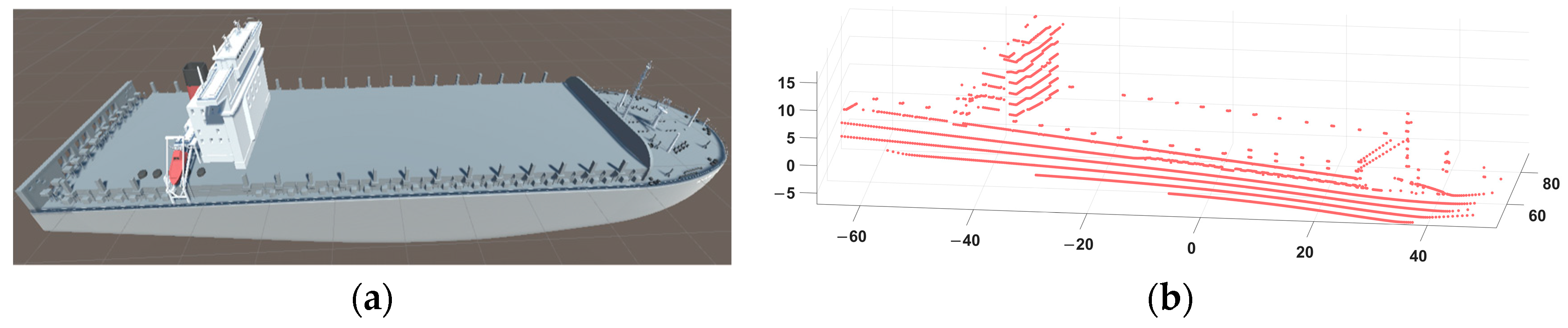
Figure 1.
Typical sufficient point cloud of a container ship: (a) represents the container ship; (b) represents the point cloud of the container ship.
Figure 1.
Typical sufficient point cloud of a container ship: (a) represents the container ship; (b) represents the point cloud of the container ship.
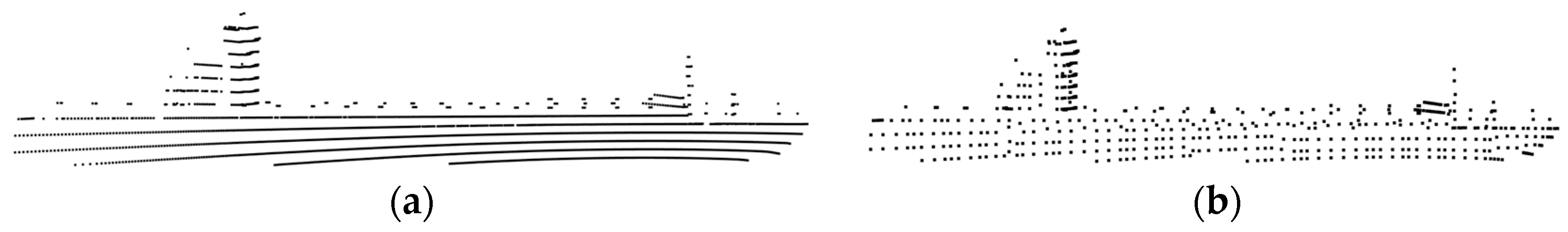
Figure 2.
Point cloud voxel filtering: (a) represents the original point cloud; (b) represents after voxel filtering.
Figure 2.
Point cloud voxel filtering: (a) represents the original point cloud; (b) represents after voxel filtering.
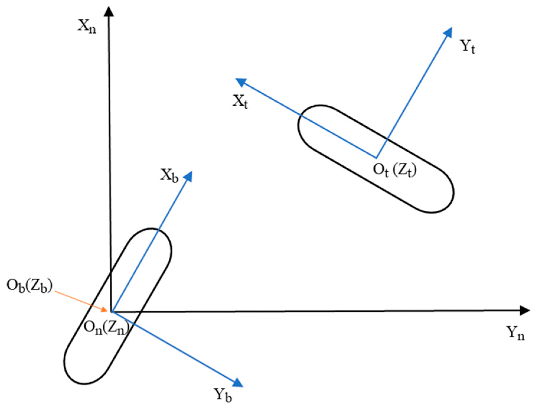
Figure 3.
The NED and BODY coordinate systems. Blue coordinates are the BODY frame and the black coordinate is the NED frame.
Figure 3.
The NED and BODY coordinate systems. Blue coordinates are the BODY frame and the black coordinate is the NED frame.
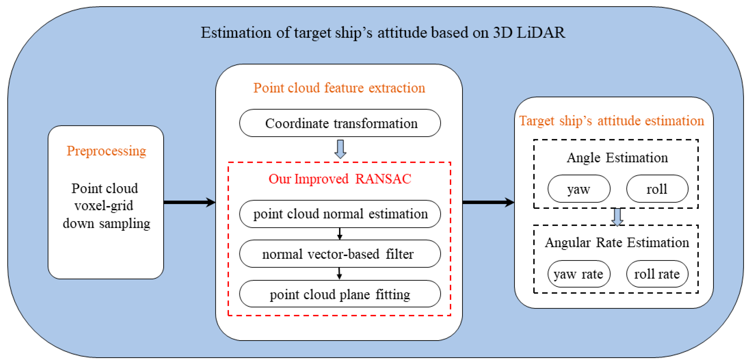
Figure 4.
Overall flow chart of our framework.
Figure 4.
Overall flow chart of our framework.
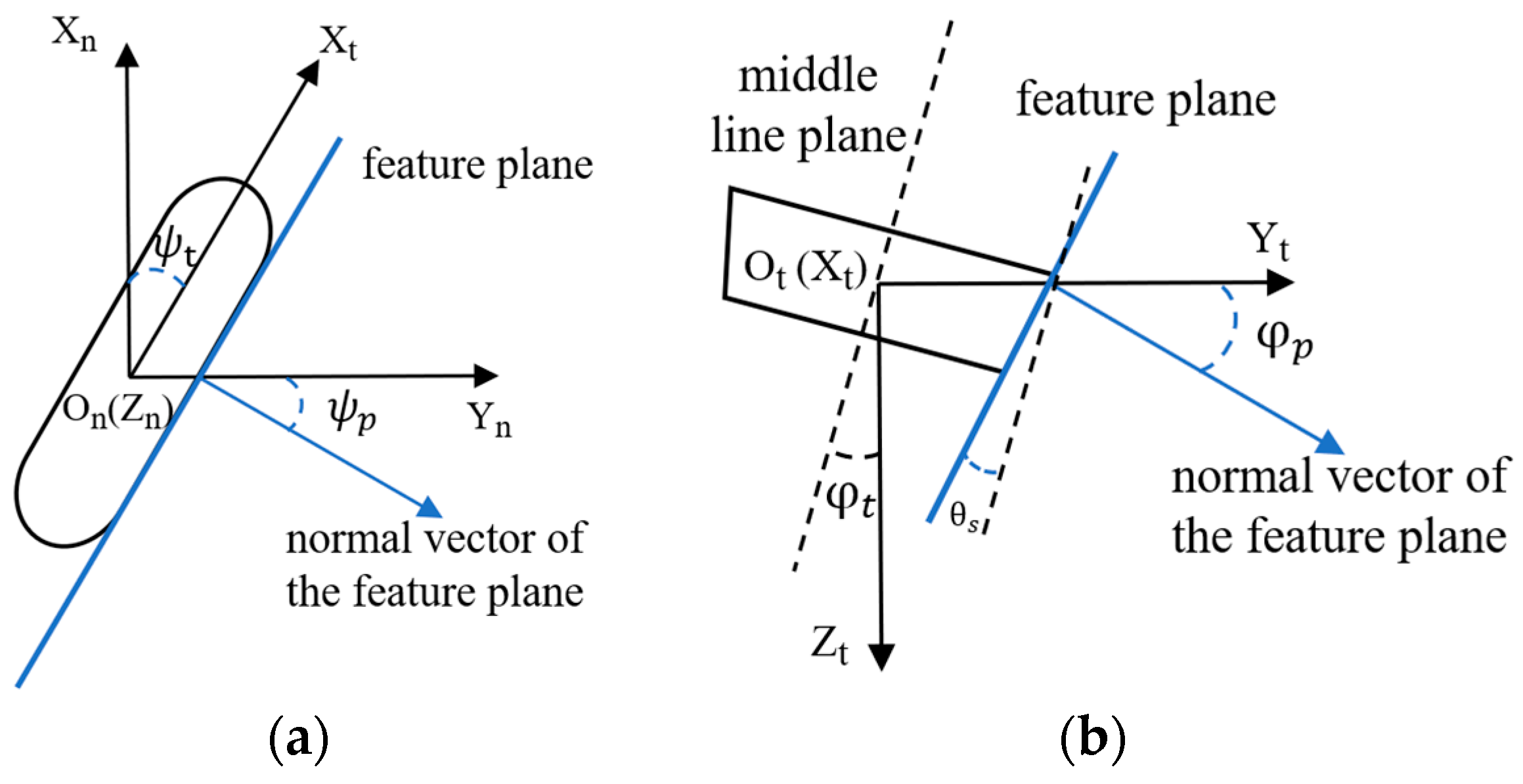
Figure 5.
The geometric relations between the feature plane and the target ship’s attitude: (a) represents the included angle in the NED frame; (b) represents the included angle and board-side inclination angle in the BODY frame.
Figure 5.
The geometric relations between the feature plane and the target ship’s attitude: (a) represents the included angle in the NED frame; (b) represents the included angle and board-side inclination angle in the BODY frame.
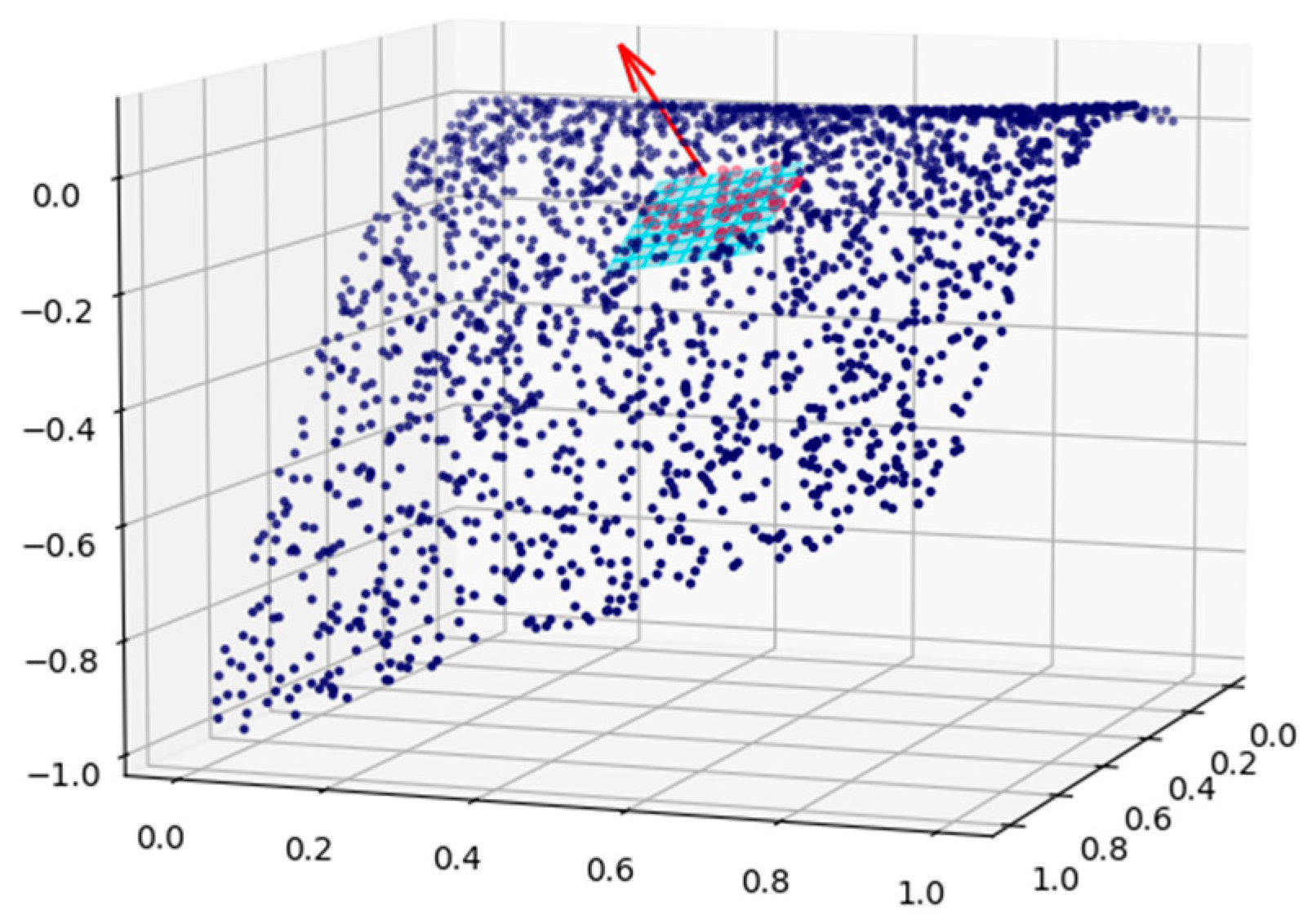
Figure 6.
The normal vector of a discrete point. The neighbor points and the normal vector are in red. The fitted plane is shown in light blue.
Figure 6.
The normal vector of a discrete point. The neighbor points and the normal vector are in red. The fitted plane is shown in light blue.
Figure 7.
Point cloud normal vector-based filtering: (a) represents the input point cloud; (b) represents after filtering.
Figure 7.
Point cloud normal vector-based filtering: (a) represents the input point cloud; (b) represents after filtering.
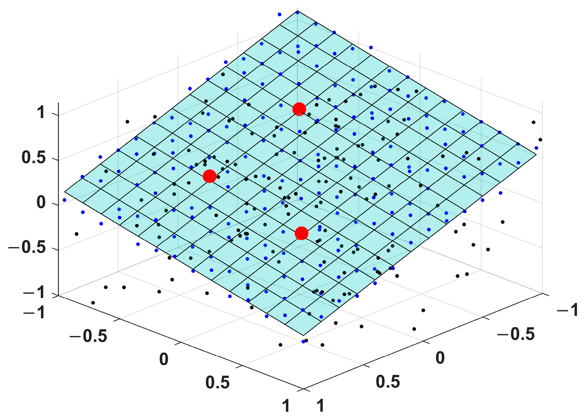
Figure 8.
The plane-fitting of RANSAC. The red points are the chosen points, the blue points are near the constructed plane, and the black points are the noise points.
Figure 8.
The plane-fitting of RANSAC. The red points are the chosen points, the blue points are near the constructed plane, and the black points are the noise points.
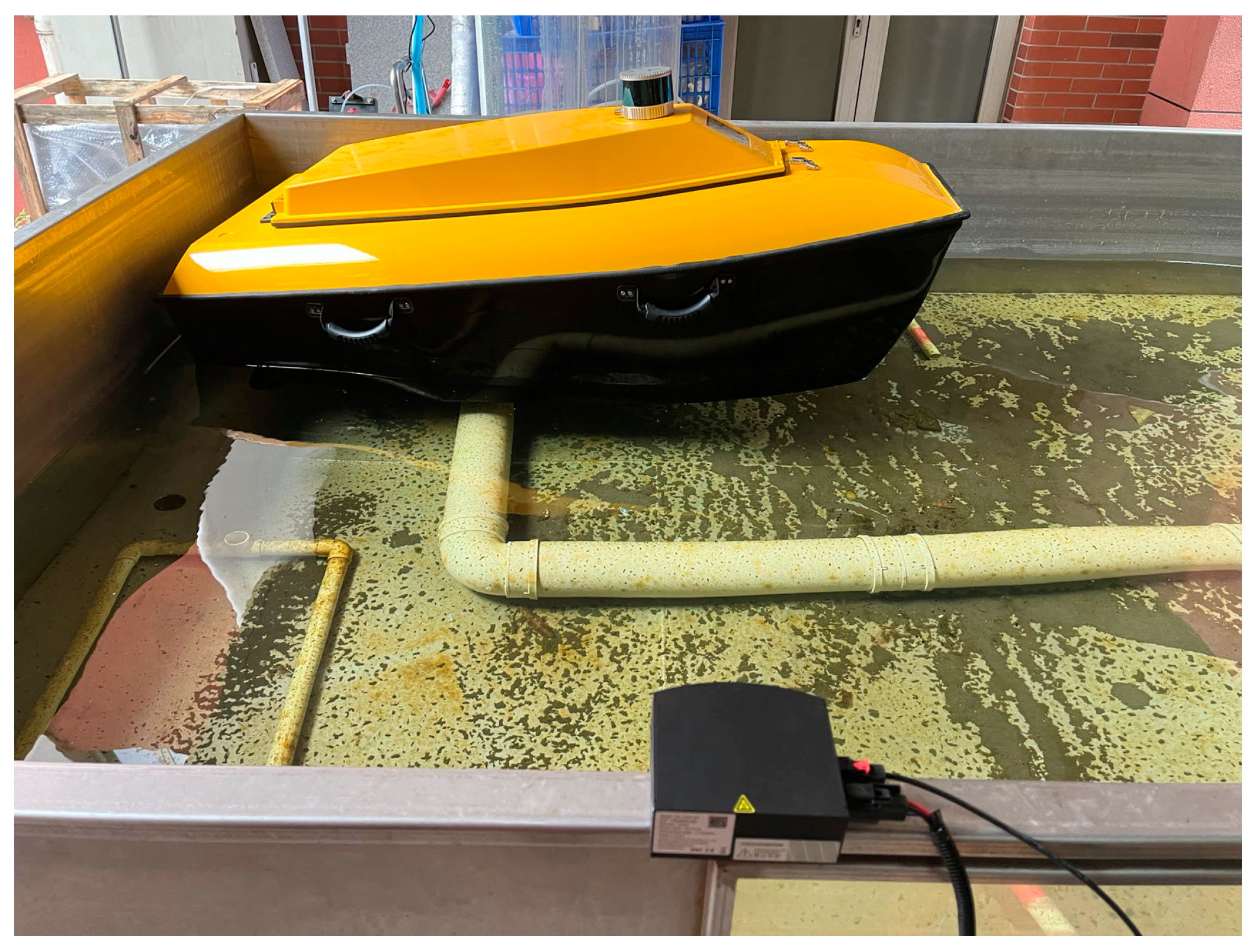
Figure 9.
The water-pool experimental scene. The USV in the upper part is “Hong Dong No. 1” and the LiDAR in the lower part is the “LS-M1” LiDAR.
Figure 9.
The water-pool experimental scene. The USV in the upper part is “Hong Dong No. 1” and the LiDAR in the lower part is the “LS-M1” LiDAR.
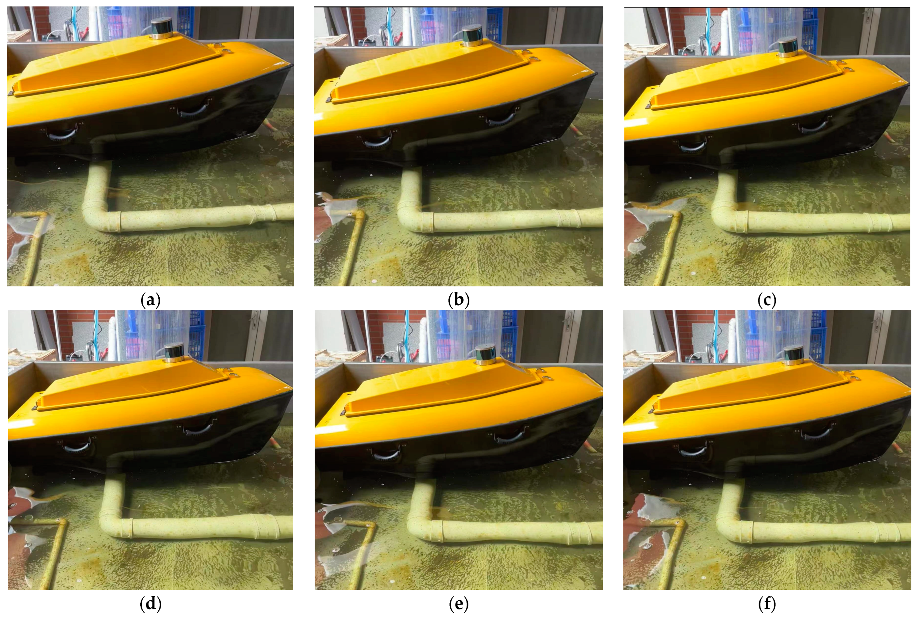
Figure 10.
The snapshots of the “Hong Dong No. 1” USV in the water-pool experiments. (a–f) is the sequence of each snapshot.
Figure 10.
The snapshots of the “Hong Dong No. 1” USV in the water-pool experiments. (a–f) is the sequence of each snapshot.
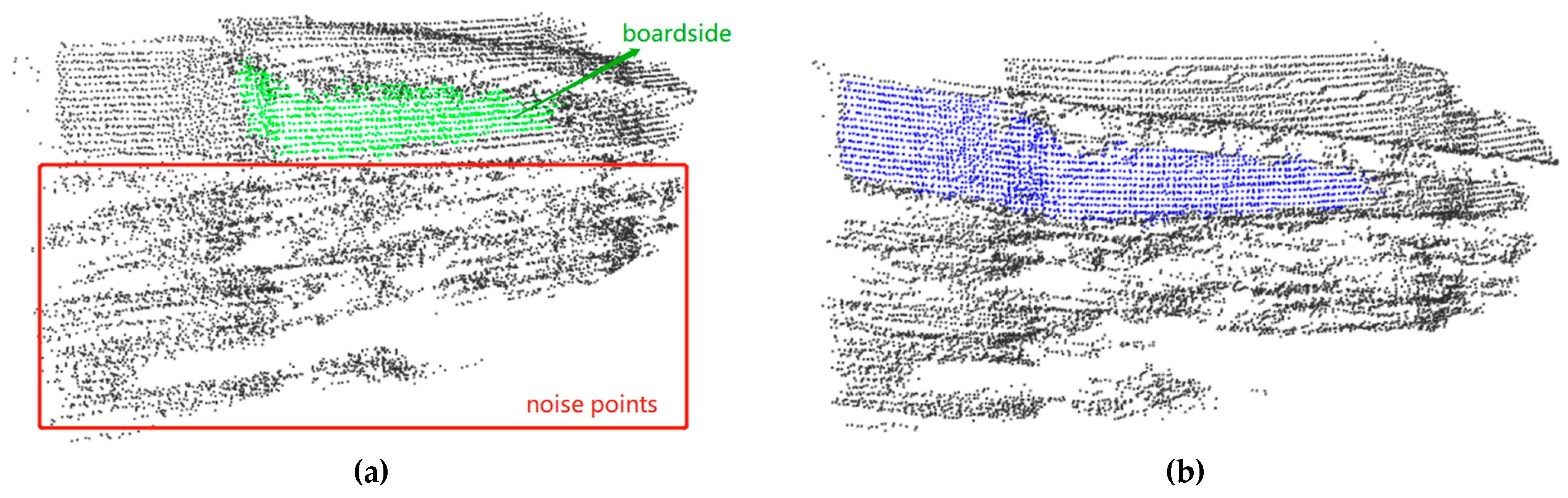
Figure 11.
The comparison of the actual raw point cloud and after filtering in the water-pool experiments: (a) represents the originally collected point cloud; (b) highlights the point cloud after our normal vector-based filter in blue.
Figure 11.
The comparison of the actual raw point cloud and after filtering in the water-pool experiments: (a) represents the originally collected point cloud; (b) highlights the point cloud after our normal vector-based filter in blue.
Figure 12.
The comparison of the feature-plane-extraction results of standard RANSAC and improved RANSAC in the water-pool experiments: (a) shows the feature-plane-extraction result of standard RANSAC; (b) shows the feature-plane-extraction result of our improved RANSAC.
Figure 12.
The comparison of the feature-plane-extraction results of standard RANSAC and improved RANSAC in the water-pool experiments: (a) shows the feature-plane-extraction result of standard RANSAC; (b) shows the feature-plane-extraction result of our improved RANSAC.
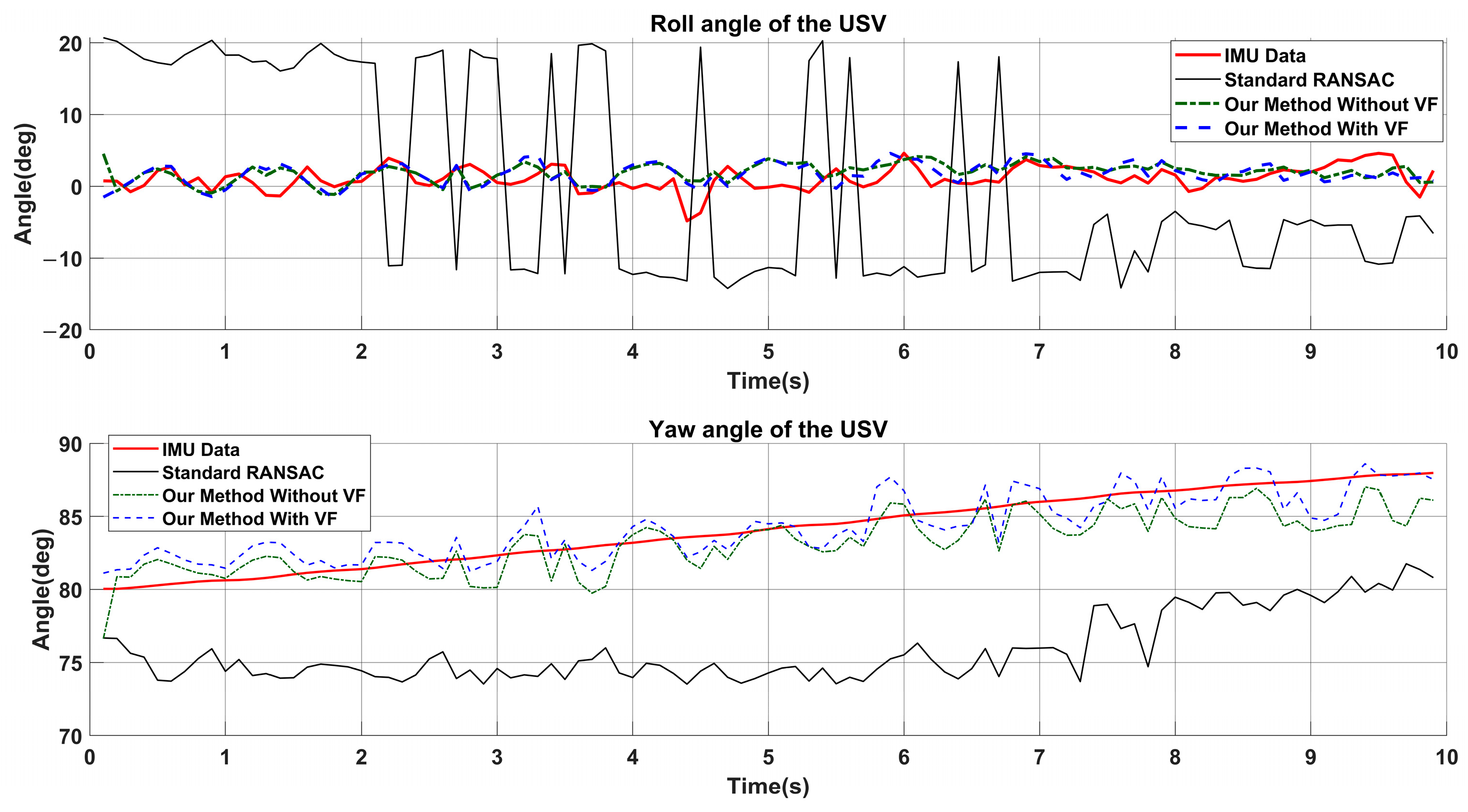
Figure 13.
The roll angle and yaw angle results in the water-pool experiments.
Figure 13.
The roll angle and yaw angle results in the water-pool experiments.
Figure 14.
The roll rate and yaw rate results in the water-pool experiments.
Figure 14.
The roll rate and yaw rate results in the water-pool experiments.
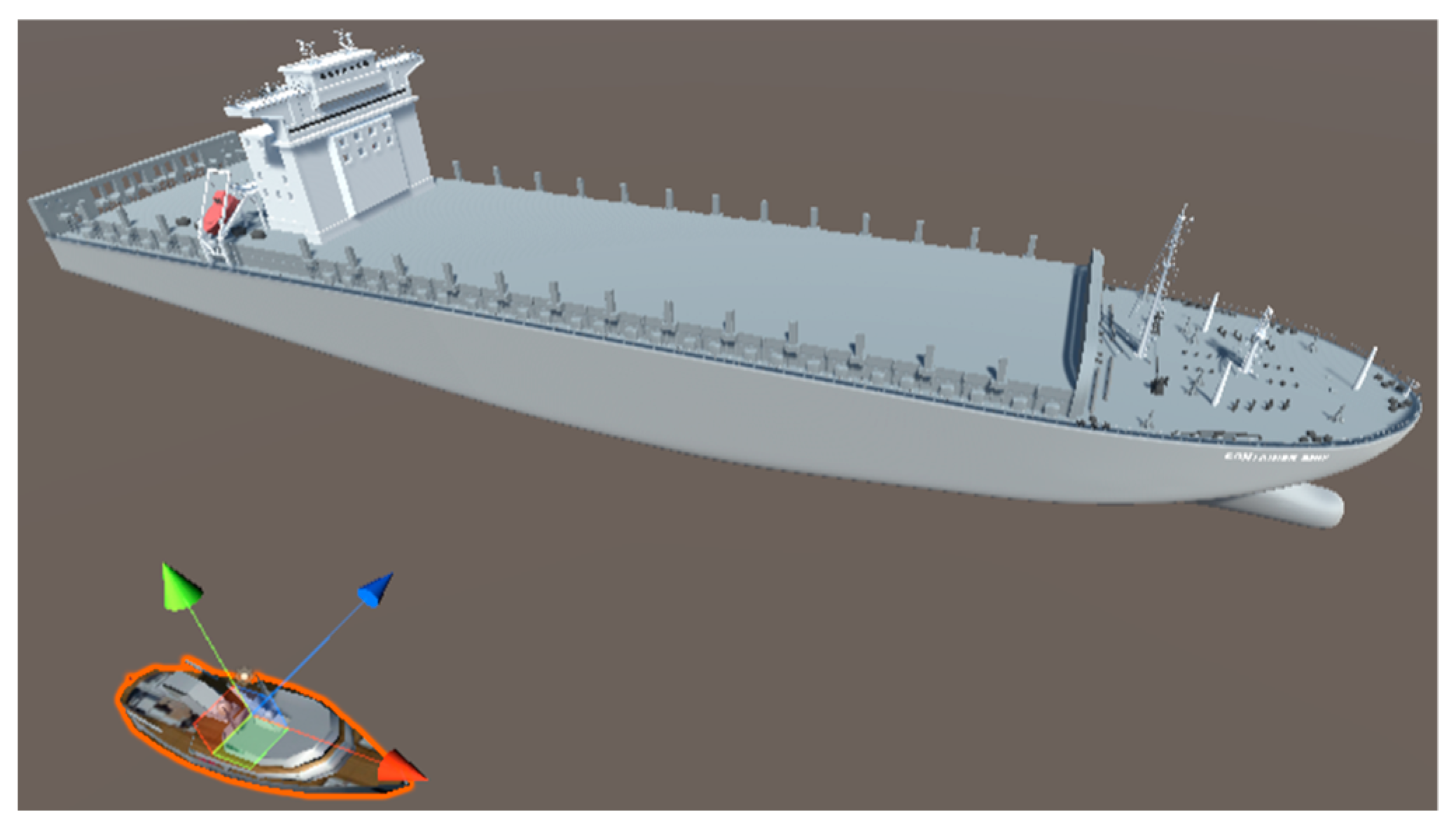
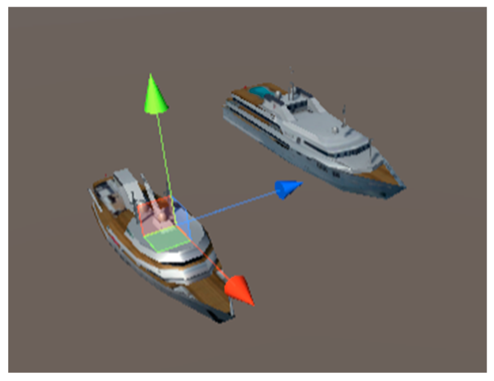
Figure 15.
The test scene of the container ship motion simulation. The coordinate arrows show the installation position of LiDAR on the observing boat.
Figure 15.
The test scene of the container ship motion simulation. The coordinate arrows show the installation position of LiDAR on the observing boat.
Figure 16.
The test scene of the yacht motion simulation. The coordinate arrows show the installation position of LiDAR on the observing boat.
Figure 16.
The test scene of the yacht motion simulation. The coordinate arrows show the installation position of LiDAR on the observing boat.
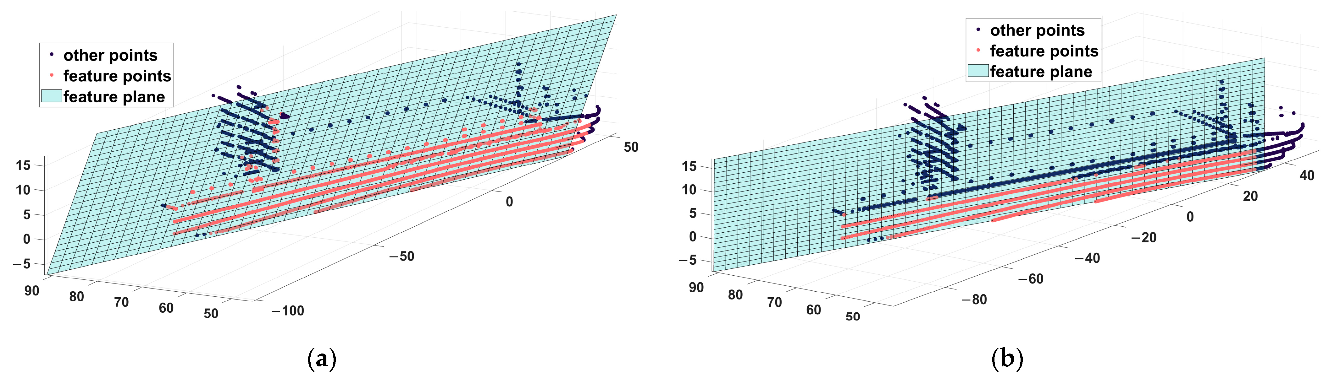
Figure 17.
The comparison of the feature-plane-extraction results of standard RANSAC and improved RANSAC in the container ship motion simulations: (a) shows the feature-plane-extraction result of standard RANSAC; (b) shows the feature-plane-extraction result of our improved RANSAC.
Figure 17.
The comparison of the feature-plane-extraction results of standard RANSAC and improved RANSAC in the container ship motion simulations: (a) shows the feature-plane-extraction result of standard RANSAC; (b) shows the feature-plane-extraction result of our improved RANSAC.
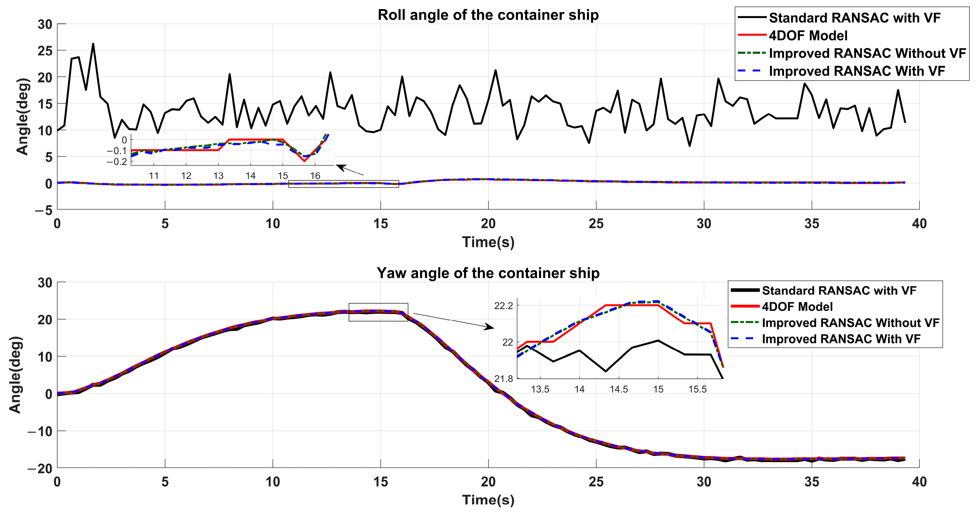
Figure 18.
The roll angle and yaw angle results in the container ship simulations.
Figure 18.
The roll angle and yaw angle results in the container ship simulations.
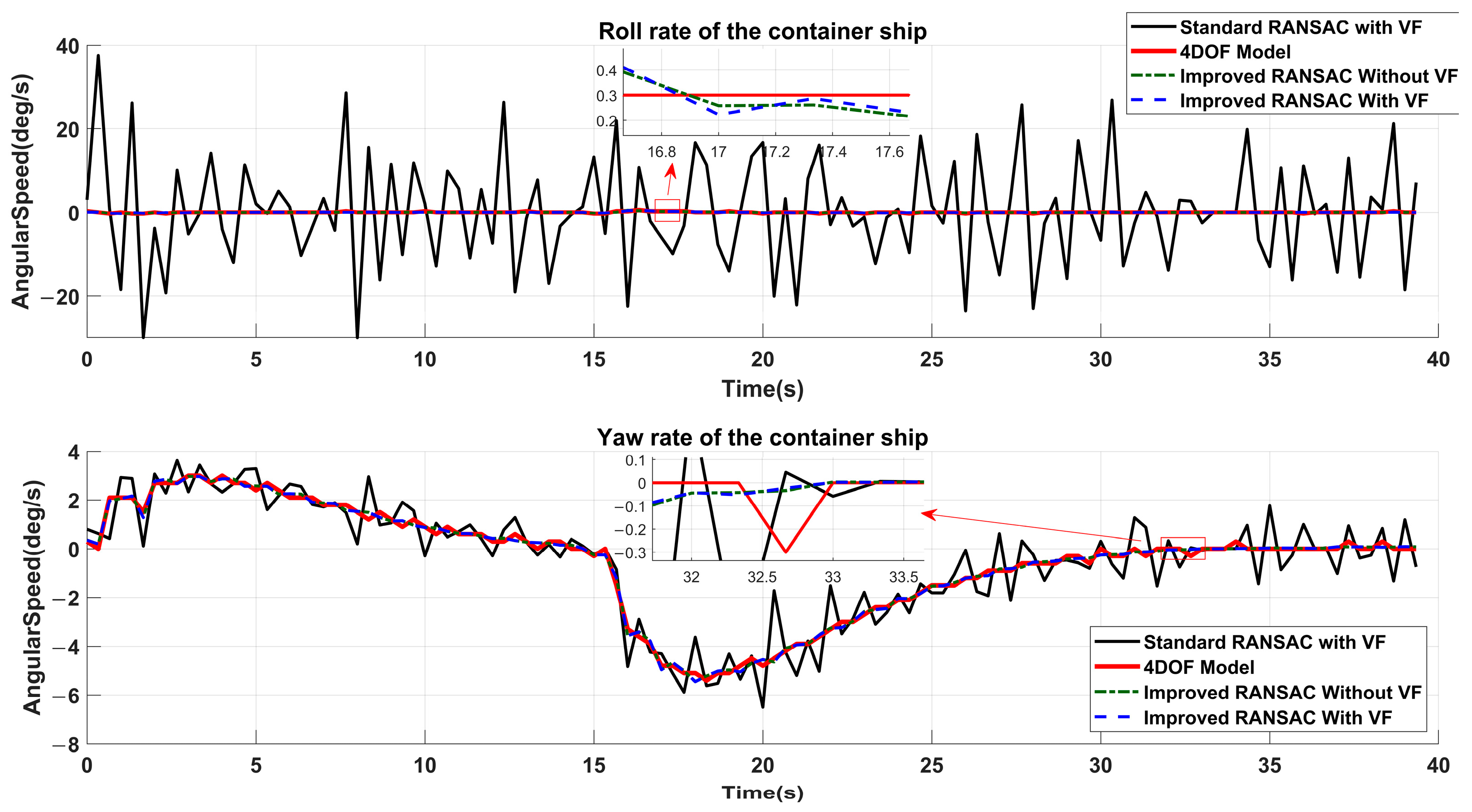
Figure 19.
The roll rate and yaw rate results in the container ship simulations.
Figure 19.
The roll rate and yaw rate results in the container ship simulations.
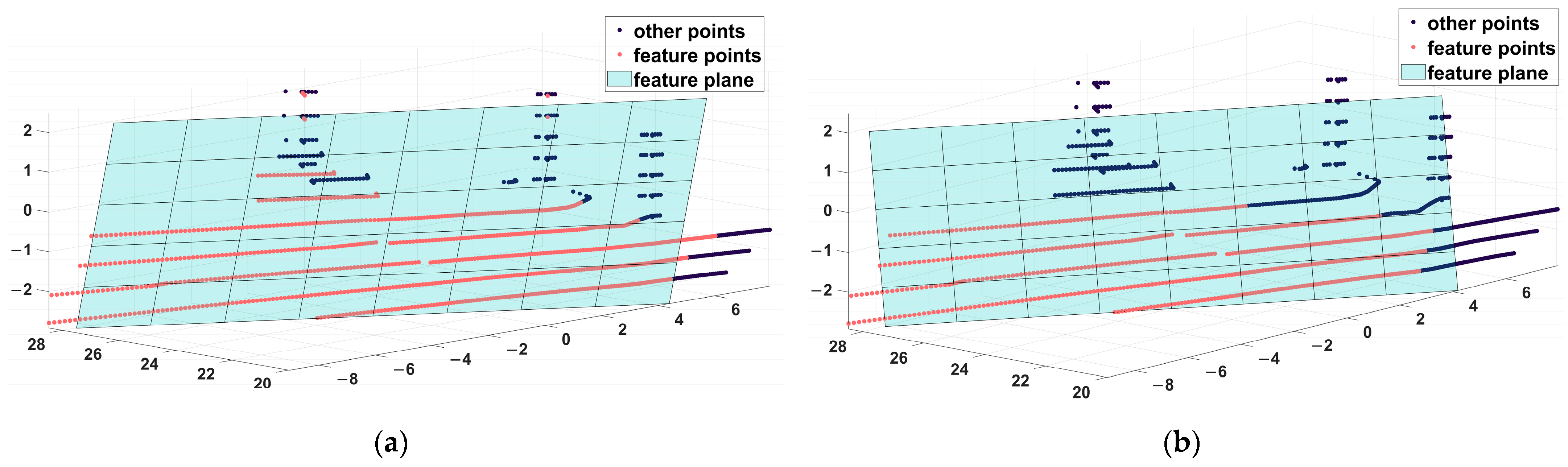
Figure 20.
The comparison of the feature-plane-extraction results of standard RANSAC and improved RANSAC in the yacht motion simulations: (a) shows the feature-plane-extraction result of standard RANSAC; (b) shows the feature-plane-extraction result of our improved RANSAC.
Figure 20.
The comparison of the feature-plane-extraction results of standard RANSAC and improved RANSAC in the yacht motion simulations: (a) shows the feature-plane-extraction result of standard RANSAC; (b) shows the feature-plane-extraction result of our improved RANSAC.
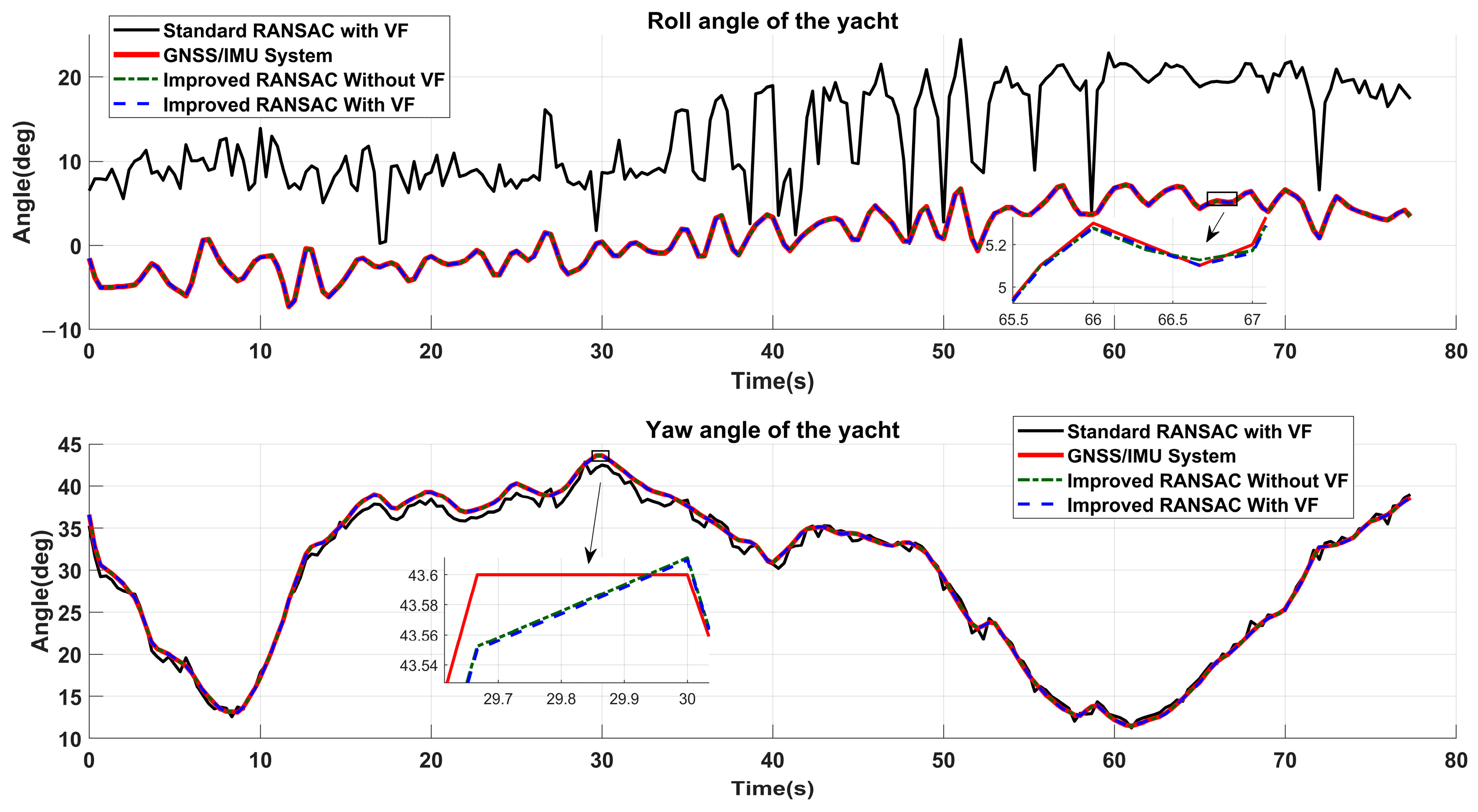
Figure 21.
The roll angle and yaw angle results in the yacht simulations.
Figure 21.
The roll angle and yaw angle results in the yacht simulations.
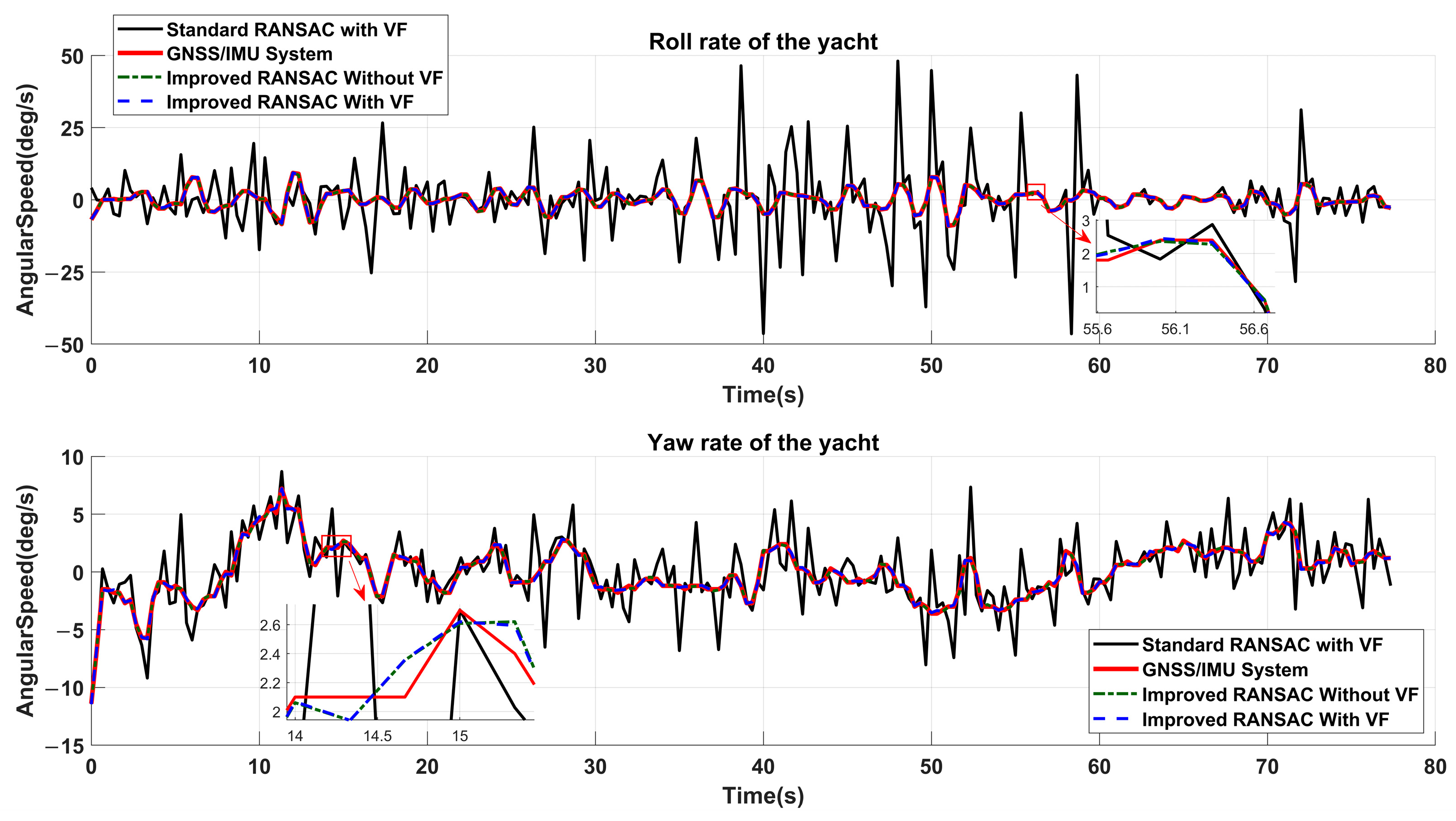
Figure 22.
The roll rate and yaw rate results in the yacht simulations.
Figure 22.
The roll rate and yaw rate results in the yacht simulations.
Table 1.
Technical information of the “LS-M1” LiDAR.
Table 1.
Technical information of the “LS-M1” LiDAR.
| Information | Value |
|---|
| maximum range | 350 m |
| laser fire frequency | 18,000 Hz |
| vertical field of view | 35 deg |
| vertical angular resolution | 0.03 deg |
| horizontal field of view | 120 deg |
| horizontal angular resolution | 0.06 deg |
Table 2.
Dimensional information of the “Hong Dong No. 1” USV.
Table 2.
Dimensional information of the “Hong Dong No. 1” USV.
| Information | Value |
|---|
| main size | 1.5 m |
| molded breadth | 0.74 m |
| molded depth | 0.6 m |
| designed draught | 0.2 m |
| board-side inclination angle | 0.1 deg |
Table 3.
The parameter settings of each method in the water pool experiment.
Table 3.
The parameter settings of each method in the water pool experiment.
| Method | Parameter | Meaning | Value |
|---|
| Improved RANSAC with VF | | Max distance of neighbor points | 0.035 m |
| Threshold of normal vector angle | 0.02 rad |
| Distance tolerance of point to plane | 0.05 m |
| Standard RANSAC with VF | | Distance tolerance of point to plane | 0.05 m |
| Improved RANSAC without VF | | Max distance of neighbor points | 0.035 m |
| Threshold of normal vector angle | 0.02 rad |
| Distance tolerance of point to plane | 0.05 m |
Table 4.
The evaluation indexes of each method in the water-pool experiments.
Table 4.
The evaluation indexes of each method in the water-pool experiments.
| Method | Attitude State | RMSE | MAE |
|---|
| Improved RANSAC with VF | Roll Angle | 2.0371° | 1.6907° |
| Yaw Angle | 1.3204° | 1.1092° |
| Roll Rate | 19.1547°/s | 15.8893°/s |
| Yaw Rate | 12.6331°/s | 8.9665°/s |
| Improved RANSAC without VF | Roll Angle | 1.9879° | 1.6301° |
| Yaw Angle | 1.2956° | 1.1068° |
| Roll Rate | 18.2154°/s | 14.3370°/s |
| Yaw Rate | 12.0684°/s | 8.8624°/s |
| Standard RANSAC with VF | Roll Angle | 14.5339° | 13.8871° |
| Yaw Angle | 8.4089° | 8.2139° |
| Roll Rate | 140.2946°/s | 75.8283°/s |
| Yaw Rate | 10.8218°/s | 7.6778°/s |
Table 5.
Technical information of the VLP-32 LiDAR.
Table 5.
Technical information of the VLP-32 LiDAR.
| Information | Value |
|---|
| laser beam | 32 |
| spinning speed | 300 RPM |
| maximum range | 200 m |
| laser fire frequency | 21,700 Hz |
| vertical field of view | 40 deg |
| horizontal field of view | 360 deg |
| horizontal angular resolution | 0.08 deg |
Table 6.
Dimensional information of the container model.
Table 6.
Dimensional information of the container model.
| Information | Value |
|---|
| main size | 125 m |
| molded breadth | 25 m |
| molded depth | 13 m |
| designed draught | 8 m |
| board-side inclination angle | 0.05 deg |
Table 7.
The parameter settings of each method in the container ship motion simulation.
Table 7.
The parameter settings of each method in the container ship motion simulation.
| Method | Parameter | Meaning | Value |
|---|
| Improved RANSAC with VF | | Max distance of neighbor points | 10 m |
| Threshold of normal vector angle | 0.003 rad |
| Distance tolerance of point to plane | 0.05 m |
| Standard RANSAC with VF | | Distance tolerance of point to plane | 0.05 m |
| Improved RANSAC without VF | | Max distance of neighbor points | 10 m |
| Threshold of normal vector angle | 0.003 rad |
| Distance tolerance of point to plane | 0.05 m |
Table 8.
Dimensional information of the yacht model.
Table 8.
Dimensional information of the yacht model.
| Information | Value |
|---|
| main size | 20 m |
| molded breadth | 6 m |
| molded depth | 3 m |
| designed draught | 1 m |
| board-side inclination angle | 0.1 deg |
Table 9.
The parameter settings of each method in the yacht motion simulation.
Table 9.
The parameter settings of each method in the yacht motion simulation.
| Method | Parameter | Meaning | Value |
|---|
| Improved RANSAC with VF | | Max distance of neighbor points | 3 m |
| Threshold of normal vector angle | 0.04 rad |
| Distance tolerance of point to plane | 0.0075 m |
| Standard RANSAC with VF | | Distance tolerance of point to plane | 0.0075 m |
| Improved RANSAC without VF | | Max distance of neighbor points | 3 m |
| Threshold of normal vector angle | 0.04 rad |
| Distance tolerance of point to plane | 0.0075 m |
Table 10.
The evaluation indexes of each method in the container ship motion simulations.
Table 10.
The evaluation indexes of each method in the container ship motion simulations.
| Method | Attitude State | RMSE | MAE |
|---|
| Improved RANSAC with VF | Roll Angle | 0.0373° | 0.0316° |
| Yaw Angle | 0.0350° | 0.0294° |
| Roll Rate | 0.1201°/s | 0.0859°/s |
| Yaw Rate | 0.1433°/s | 0.1163°/s |
| Improved RANSAC without VF | Roll Angle | 0.0377° | 0.0307° |
| Yaw Angle | 0.0349° | 0.0293° |
| Roll Rate | 0.1088°/s | 0.0766°/s |
| Yaw Rate | 0.1430°/s | 0.1162°/s |
| Standard RANSAC with VF | Roll Angle | 13.9727° | 13.5472° |
| Yaw Angle | 0.2845° | 0.2383° |
| Roll Rate | 13.0475°/s | 10.0682°/s |
| Yaw Rate | 0.8129/s | 0.6323°/s |
Table 11.
The evaluation indexes of each method in the yacht motion simulations.
Table 11.
The evaluation indexes of each method in the yacht motion simulations.
| Method | Attitude State | RMSE | MAE |
|---|
| Improved RANSAC with VF | Roll Angle | 0.0466° | 0.0368° |
| Yaw Angle | 0.0365° | 0.0295° |
| Roll Rate | 0.1942°/s | 0.1513°/s |
| Yaw Rate | 0.1362°/s | 0.1090°/s |
| Improved RANSAC without VF | Roll Angle | 0.0440° | 0.0346° |
| Yaw Angle | 0.0363° | 0.0292° |
| Roll Rate | 0.1843°/s | 0.1449°/s |
| Yaw Rate | 0.1354°/s | 0.1083°/s |
| Standard RANSAC with VF | Roll Angle | 12.7396° | 12.2805° |
| Yaw Angle | 0.8079° | 0.6695° |
| Roll Rate | 11.5327°/s | 6.9814°/s |
| Yaw Rate | 2.1816°/s | 1.5662°/s |
Table 12.
The average evaluation indexes 1 of each method.
Table 12.
The average evaluation indexes 1 of each method.
| Attitude State | Method | Average RMSE | Average MAE |
|---|
| Roll Angle (°) | Improved RANSAC with VF | 0.7070 | 0.5864 |
| Improved RANSAC without VF | 0.6899 | 0.5651 |
| Standard RANSAC with VF | 13.7487 | 13.2383 |
| Yaw Angle (°) | Improved RANSAC with VF | 0.4640 | 0.3894 |
| Improved RANSAC without VF | 0.4556 | 0.3884 |
| Standard RANSAC with VF | 2.9247 | 3.0406 |
| Roll Rate (°/s) | Improved RANSAC with VF | 6.4897 | 5.3755 |
| Improved RANSAC without VF | 6.1695 | 4.8528 |
| Standard RANSAC with VF | 54.9583 | 30.9593 |
| Yaw Rate (°/s) | Improved RANSAC with VF | 4.3042 | 3.0639 |
| Improved RANSAC without VF | 4.1156 | 3.0290 |
| Standard RANSAC with VF | 4.6054 | 3.2921 |
Table 13.
The angle and angular rate average evaluation indexes 1 and reduction percentage.
Table 13.
The angle and angular rate average evaluation indexes 1 and reduction percentage.
| Attitude State | Method | Average RMSE | Average MAE |
|---|
| Angle | Improved RANSAC with VF | 0.5855° | 0.4879° |
| Standard RANSAC with VF | 8.3367° | 8.1395° |
| Reduction Percentage 2 | 91.62% | 92.93% |
| Angular Rate | Improved RANSAC with VF | 5.3970°/s | 4.2197°/s |
| Standard RANSAC with VF | 29.7819°/s | 17.1257°/s |
| Reduction Percentage 2 | 71.81% | 75.36% |


