1. Introduction
The advancement of affordable, long-range autonomous marine vehicle (AMV) technologies, including unmanned surface vehicles (USVs), autonomous underwater vehicles (AUVs), underwater gliders, and wave gliders [
1], has presented opportunities for the deployment of persistent, robotic, and autonomous Lagrangian networks in ocean environment sensing. In contrast to conventional ocean observation networks such as the ARGO array [
2], the utilization of mobile and autonomous networks composed of a collection of AMVs offers a distinctive technical capability: controllable maneuverability in complex and dynamic ocean environments. Therefore, effectively leveraging their controllable maneuverability to enable the networks to acquire cost-effective and information-rich sensing data within nonuniform and dynamic ocean environments, aligning with the requirements of observation missions, is a key issue within the research community focused on autonomous ocean sensing with AMV networks.
The tracking of dynamic ocean features to gather in situ data for characterizing and predicting the evolution of these features, such as thermoclines [
3], plumes [
4], and mesoscale eddies [
5], is an aspect of applying AMV networks for ocean sensing. Besides feature tracking, a foundational application objective in utilizing AMV networks is to autonomously and adaptively collect a variety of informative Lagrangian data streams, such as temperature, salinity, and flow velocity of seawater, that can be assimilated into predictive ocean models. The assimilation of these data streams can lead to significant improvement in the accuracy of temporal predictions for spatial fields in ocean environments [
6]. Consequently, the real-time optimization of the data streams for assimilation using numerical ocean models is crucial in maximizing model prediction performance, and it plays an essential role in both research and practical applications of ocean sensing with AMV networks. One key approach to addressing this optimization problem is through the utilization of feedback control theory and the formulation of a sensor management technical framework [
7]. This framework establishes a closed-loop system by integrating a numerical ocean model with an AMV sensing network [
8] and uses iterative feedback and optimization processes to continuously adapt the network’s sensing strategies and improve prediction performance. Different from conventional feedback control of dynamic systems, the feedback control in the closed-loop adaptive ocean sensing and prediction system involves cooperative control of the sensing actions of the networked AMVs, taking into account the constraints imposed by ocean environments. And the primary objective of this feedback control is to collect informative sensing data of ocean environments, which can be utilized in ocean models to improve prediction performance. The AOSN II and ASAP projects have made significant contributions to the research on autonomous and adaptive ocean sensing with AMV networks, particularly regarding the utilization of underwater gliders as part of the sensing network [
9,
10]. These projects have laid an important foundation for the further advancements in this field.
In the context of ocean sensing and prediction systems, predictive ocean models play an important role. Alongside traditional methods based on numerically solving partial differential equations of geophysical fluid dynamics, data-driven techniques have emerged as powerful and complementary tools for ocean modeling and prediction. Leveraging machine learning and statistical approaches, data-driven methods extract patterns and relationships from observed data, enabling them to make high-resolution and accurate predictions with reduced computational costs. Extensive research efforts have been dedicated to developing and applying data-driven techniques for ocean modeling and spatial and temporal predictions. Notable approaches include objective analysis (OA) [
11,
12], Gaussian process (GP) [
13], Kriging geostatistical prediction [
14], compressive sensing [
15], radial basis functions (RBFs) [
16], proper orthogonal decomposition [
17,
18], dynamic mode decomposition (DMD) [
19], and neural networks [
20,
21]. Compared to conventional ocean models, data-driven techniques rely more heavily on the information content within the data for their implementation. Building upon the aforementioned data-driven techniques, researchers have devised methodologies to optimize sensing strategies for both Eulerian and Lagrangian platforms, as demonstrated in [
11,
12,
13,
16,
17,
18]. These optimized strategies enable the collection of informative data, leading to enhancements in data-driven prediction performance. Through the integration of data-driven techniques and adaptive observation strategies within the closed-loop system, the ocean sensing and prediction capabilities of AMVs can be significantly improved. This approach holds great potential in achieving high-resolution and accurate ocean prediction with AMV sensing networks.
High-resolution and accurate flow field prediction is a fundamental component in ocean prediction. The spatiotemporal flow information not only offers insights into the multi-scale dynamic behavior of ocean currents but also plays a crucial role in path planning [
22,
23], navigation [
24,
25], feature prediction and tracking [
26], and motion control for both individual and swarms of AMVs [
11,
27] implementing ocean sensing missions. Many studies have been conducted on data-driven flow prediction [
22,
24,
25,
28,
29,
30], addressing flow prediction in diverse oceanic environments where tidal or non-tidal flow is dominant. However, a research gap exists in the specific area of integrating data-driven flow modeling, online data assimilation of flow sensing data into data-driven flow models, and optimizing AMVs’ flow sensing strategy, based on the closed-loop feedback ocean prediction and adaptive sensing technical framework.
Based on the above review and discussions, as well as recognizing the significance of high-resolution and accurate flow field prediction in ocean prediction and AMVs’ operations, this article is dedicated to exploring this data-driven closed-loop approach and systematically developing methods for data-driven flow modeling, data assimilation, and optimizing AMVs’ observations. The systematic development establishes a dynamic data-driven application system (DDDAS) [
31] for flow prediction and sensing with AMVs. The DDDAS seamlessly integrates data-driven modeling, data assimilation, and an optimal decision-making process, as depicted in
Figure 1, thereby enhancing high-resolution and accurate flow field prediction capabilities and enabling adaptive and efficient flow sensing using AMVs.
The main contributions and novelties of this article are as follows: (1) Pioneering closed-loop DDDAS development: This article represents an advancement by introducing the first-ever closed-loop data-driven DDDAS designed for predicting flow fields. The system seamlessly integrates data-driven flow modeling, data assimilation, and adaptive sensing with AMVs. (2) A hybrid data-driven flow model: This article proposes an innovative hybrid data-driven flow model that combines the predictive power of a neural network with the statistical estimation of a Gaussian process model. Notably, the neural network architecture is designed to incorporate prior knowledge of tidal components, contributing to accurate flow predictions. This hybrid model not only captures flow trends accurately but also effectively handles residuals. (3) The Kriged ensemble transform Kalman filter (ETKF) data assimilation: This article introduces a pioneering application of the Kriged ETKF method for assimilating spatially correlated flow-sensing data from AMVs. This methodology demonstrates exceptional efficacy in model learning and spatiotemporal flow prediction. It also enhances the optimization of AMVs’ sensing paths. (4) A receding horizon strategy for optimal path planning: Addressing the challenge of non-myopic optimal path planning for a network of AMVs, this article introduces a strategic receding horizon approach. To tackle the resulting computational complexity of large-scale tree-searching-based optimization, this article proposes a novel distributed Monte Carlo Tree Search (MCTS) method. This innovative approach harnesses the collective computational capabilities of networked AMVs to explore the search space and derive effective planning solutions.
The rest of this paper is structured as follows.
Section 2 presents the data-driven hybrid flow model, including the neural network model and the Gaussian process model.
Section 3 elaborates on the state and observation models for data assimilation and the implementation of the Kriged ETKF method for model learning and flow prediction.
Section 4 presents the optimization of the AMVs’ paths for collecting informative flow-sensing data to enhance flow prediction accuracy.
Section 5 presents simulation studies to demonstrate the performance of the DDDAS. Finally,
Section 6 presents the conclusions.
2. Data-Driven Flow Prediction Model
The flow model serves as a fundamental component within the developed DDDAS. The section introduces the developed hybrid data-driven model, which leverages the machine learning model of neural networks and the statical model of the Gaussian process.
Section 2.1 provides an overview of the hybrid model.
Section 2.2 presents the utilization of the tidal harmonic analysis method to extract essential prior knowledge of the flow, supporting the design of the neural network model.
Section 2.3 elaborates on the development of the neural network model and
Section 2.4 presents the Gaussian process model.
2.1. Model Overview
To enable the prediction of the flow speed at specific spatiotemporal locations
, where
represents the spatial location and
represents the time, a data-driven spatiotemporal flow field model is established. This model comprises two submodels:
Equation (1) represents the submodel for the latitudinal flow speed , and Equation (2) represents the submodel for the longitudinal flow speed , at the given spatiotemporal locations .
The flow model consists of two fundamental components: the mean component, and the residual component. The mean component, denoted as
and
, captures the average or expected flow speeds, providing the trends in flow at the given spatiotemporal location. In this article, a feedforward neural network is employed to approximate the continuous and nonlinear function of
and
. The choice is motivated by the neural network’s universal approximation capabilities, which enable it to effectively learn and represent the complex relationships between input parameters including longitude, latitude, time, and the corresponding flow speed. To implement the flow model, a specific neural network is designed, and its detailed architecture is described in
Section 2.3. On the other hand, the residual component, denoted as
and
, accounts for variations from the mean component. These residuals may arise due to unmodelled influences or other factors affecting the flow speed. In this article, the Gaussian process is employed to model
and
, which will be described in detail in
Section 2.4. The composition of the flow prediction model, take
for example, is depicted in
Figure 2. By decomposing the flow into mean and residual components, the spatiotemporal flow model could effectively capture both the average behavior and the deviations from the average, which enhance the accuracy and reliability of the predictions.
Throughout the subsequent sections, the model for will be focused on as an example for description and discussion. And to simplify expression and notation, the subscript in and will be omitted. It is important to note that both and share the same structural components and underlying principles. Therefore, the descriptions, methodologies, and discussions related to can be directly applied to .
2.2. Decomposition of Flow Using Tidal Harmonic Analysis
Driven by tidal forces, flow fields in nearshore ocean environments often exhibit spatiotemporal periodic features, which can be characterized by the presence of multiple periodic components. These components possess distinct frequencies and amplitudes, playing significant roles in shaping the overall flow dynamics. Incorporating information about the tidal components in the design of the neural network architecture allows for capturing and learning about the relationships between the tidal components and the flow speed more effectively. Therefore, this article implements this integration of knowledge of tidal components into the neural network design, leveraging the periodic patterns present in the flow field to enhance the accuracy of flow prediction.
Tidal harmonic analysis is an effective approach for decomposing the flow into different constituents, represented by trigonometric functions with distinct frequencies. It processes the training data of a temporal sequence of flow fields to identify the dominant tidal frequencies and their corresponding amplitudes. The tidal frequencies can be calculated using methods such as least-squares harmonic estimation (LS-HE) [
32] and multivariate LS-HE [
33]. Once the frequencies are determined, the amplitudes and phases of the corresponding trigonometric function for each tidal constituent can be calculated using methods such as least-squares estimation. These constituents capture the fundamental periodic components of the flow.
In this article, the tidal harmonic analysis is implemented to obtain the tidal constituents. Each obtained tidal constituent corresponds to two orthogonal temporal basis functions, given by:
where
represents the period of the
-th tidal constituent, and
represents the total number of the chosen dominant constituents. These basis functions form a basis set that captures the periodic variations in the flow over time.
For a specific spatial location
, the flow contributed by the
-th tidal constituent can be expressed as follows:
where the coefficients
and
represent the amplitudes of the basis functions
and
at location
, respectively. Considering the contributions of all tidal constituents, the overall flow at the spatial location
can be expressed as:
where
represents the non-tidal constant component of the flow at spatial location
,
varies with the locations, and
.
2.3. Neural Network Model for the Mean Component
Based on the flow model in Equation (5), a feedforward neural network is designed to model
in this article, and its architecture is depicted in
Figure 3. The main objective of the network is to learn about the relationship between
and
, enabling the prediction of the flow field.
In the model, the neural network takes the latitudinal coordinate and the longitudinal coordinate of the spatial location , along with the time as input parameters. It then outputs the predicted flow speed at . The neural network consists of three hidden layers: the -layer, the -layer, and the -layer. The -layer consists of nodes that are fully connected to the model inputs and . The -layer has nodes that are fully connected to the -layer. And the -layer is a hidden multiplicative layer with nodes, which is connected to the model input . The model output is obtained by calculating the inner product of the outputs from the -layer and the -layer. The parameters of the neural network are denoted as follows: the connection weight matrix between the -layer nodes and the input nodes is denoted as , and the bias vector of the -layer nodes is denoted as . Similarly, the connection weight matrix between the -layer nodes and the -layer nodes is denoted as , and the bias vector of the -layer nodes is denoted as . Additionally, the connection weight between the node and the node is denoted as , and the bias of the node is denoted as , where ranges from to , and ranges from to .
To introduce nonlinearity into the neural network, the -type hyperbolic tangent function is selected as the activation function for the -layer, i.e., . For the -layer, the linear activation function is chosen, i.e., . The temporal basis functions are chosen as the corresponding activation functions for the -layer.
For the offline learning of the network parameters using the data of flow and its learned tidal constituents, the Levenberg–Marquardt backpropagation optimization method is employed. This optimization technique efficiently adjusts the connection weights and biases of the neural network to minimize the mean squared error function, which is chosen as the objective function. Once the network is trained, it can effectively predict the flow field at new spatiotemporal locations using the learned relationships from the training data.
2.4. Gaussian Process Model for the Residual Component
In this article, the residual component of the flow model is modeled using a Gaussian process model. GPs, renowned in machine learning and statistics, prove invaluable for representing complex data relationships and providing predictions along with uncertainty estimations. In this article, the Gaussian process model adopts a zero mean and an assumption is made that in the model the residuals do not exhibit temporal dependencies, meaning that they are temporally uncorrelated, thus . This assumption allows the model to capture the spatial correlation between flow measurements at different spatial locations.
In the model, the kernel function
quantifies the covariance between the spatiotemporal locations
and
, thereby measuring the similarity or dissimilarity between the flow at different spatiotemporal locations. Here,
represents the expectation operator. In this article, the anisotropic squared exponential kernel function is selected to describe the spatial correlation of the residual component of the model at time
:
Here, , , and are the model hyper-parameters at time , where is the overall variance, is the latitudinal length scale, and is the longitudinal length scale. And represents the vector of the model hyper-parameters.
The accuracy of the hyper-parameters
significantly impacts the prediction accuracy of the model. To estimate the model hyper-parameters
, the maximum likelihood estimation method is employed. This estimation method uses the available data at time
to find the hyper-parameters that maximize the likelihood of the observed residuals. The implementation details of this estimation process are provided in
Section 3.5.
It should be noted that the modeling performance can be further enhanced by employing more advanced and sophisticated kernel functions. This article, however, focuses on the widely used anisotropic squared exponential kernel function. Comparisons involving different kernel functions fall beyond the scope of this article.
3. Data Assimilation with the Kriged ETKF
To achieve accurate predictions of flow speeds using the presented flow model, it is essential to accurately estimate the model parameters, including the weights and biases in the neural network model, as well as the hyper-parameters in the residual model. While the parameters of the flow model can be learned from historical data, there are limitations and uncertainties associated with the data used for training. These challenges include data sparsity, noise, and discrepancies in the actual flow conditions that the model aims to predict. To address these issues and improve the accuracy of flow predictions, this article implements online real-time learning of the parameters of the model using in situ sensing data of flow speeds provided by AMVs, employing the sequential Bayesian filtering method. This real-time learning enables the model to adapt to changing conditions to closely align with the actual flow conditions and to refine its predictions based on the most recent observations, thereby leading to more accurate and reliable predictions of flow in nearshore ocean environments.
This section delves into the implementation of data assimilation, a crucial aspect of the developed DDDAS.
Section 3.1 and
Section 3.2 provide the state model and observation model, respectively, which serve as the foundation for the subsequent implementation of the sequential data assimilation process.
Section 3.3 presents the learning of the neural network model using the ETKF method, and
Section 3.4 presents the flow field prediction using contributions from both the learned neural network model and the Gaussian process model. Finally,
Section 3.5 addresses the estimation of the hyper-parameters within the Gaussian process model, thereby completing the comprehensive data assimilation process with the Kriged ETKF method.
3.1. State Model
For the neural network model, all the connection weights
, as well as all the biases
, play a crucial role in establishing the nonlinear regression relationship between
and
for the spatiotemporal flow field model. These model parameters are selected as model state variables. And the model state vector, denoted as
, consists of all model state variables, represented as follows:
And the temporal state evolution is assumed to be driven by white noise, and it conforms to the following equation:
In this equation, represents the posterior analysis state at the previous time step , which is the estimated state based on the available observations up to time step , represents the forecast state at time step based on , and represents the Gaussian white process noise at time step .
3.2. Observation Model
This section describes the observation model for the implementation of the online learning with the sequential Bayesian filtering method, which establishes the relationship between the observed flow speeds from AMVs and the underlying state variables.
Assuming that there are
flow speed observations
at
spatial locations
by
AMVs, and the
-dimensional observation vector
at time
for all the
spatial locations is given by:
where
is the true flow speed at time
for all
spatial locations, and
is the observation noise at
.
follows a Gaussian distribution with zero-mean vector and covariance matrix
, where
is the observation noise variance, and
is the
-dimensional identity matrix.
In Equation (9), the mean component
of
can be expressed as follows:
where
is the observation matrix. The observation matrix maps the flow from the model state space to the observation space at
for all
spatial observation locations and is defined based on the architecture of the neural network as follows:
where
, and
, in which
and
.
Based on the above equations, the measurement equation can be expressed as follows:
3.3. Filtering with ETKF
Based on the structure of the presented flow model and the need for model learning and flow prediction using flow speed data from AMVs, this article employs the Kriged Kalman filter method [
34] to implement the data assimilation and flow prediction. The Kriged Kalman Filter integrates Kriging’s spatial interpolation capabilities and the Kalman filter’s optimal state estimation to effectively combine spatial correlations and temporal dynamics. In the DDDAS system, the data assimilation process not only improves flow predictions but also supports the optimization of AMVs’ observation strategies. To achieve this, the Kriged ETKF is introduced. The implementation of the Kriged ETKF is detailed as follows, and the optimization strategy which further enhances the model’s predictive capabilities will be elaborated on in
Section 4.
In the ensemble-based filtering approach, a total of
ensemble members are considered. The initial model state vector is perturbed to generate the initial ensemble of the model state vectors
. These perturbations introduce variability and diversity in the initial state estimates, which is crucial for robust data assimilation. The forecast equation then drives the evolution of each ensemble member over time as follows:
where
represents the forecast ensemble at
,
is the perturbed posterior analysis ensemble at
, and
is the ensemble of forecast noise at
, where
is the total number of model state variables. This noise follows a Gaussian distribution with a zero-mean vector and a covariance matrix
.
By subtracting the forecast ensemble mean from each ensemble member, the forecast ensemble perturbations matrix at
can be obtained as follows [
35]:
where
is the mean forecast state at
, which is defined as the ensemble mean of the forecast state as follows:
The forecast error covariance matrix at
can be obtained as follows:
where
represents the forecast error covariance matrix at time
, and
is the forecast ensemble perturbations matrix as defined in Equation (14). The forecast error covariance matrix provides a measure of uncertainty in the forecast state, which is essential for accurately estimating the flow field and making reliable predictions.
The mean posterior analysis state at time
can be obtained as follows:
where
represents the Kalman gain matrix at time
as follows:
and
is the observation error covariance matrix at time
given by:
where
is the residual vector at time
, and
is the
-dimensional identity matrix.
The ETKF [
35] introduces a transformation matrix that efficiently transforms the forecast ensemble perturbations into the posterior analysis ensemble perturbations, thereby reducing the complexity of the posterior analysis state calculation. At time
, the transformation matrix is given by:
where
is a matrix containing all the orthogonal eigenvectors of the matrix
,
is a diagonal matrix with all corresponding eigenvalues as its main diagonal elements, and
is the
-dimensional identity matrix. This transformation matrix plays a crucial role in the data assimilation process by efficiently adjusting the forecast ensemble perturbations to be consistent with the observations, leading to more accurate and reliable posterior analysis state estimates.
The posterior analysis ensemble perturbations matrix at time
can be obtained by applying the transformation matrix
as follows [
35]:
By adding the mean posterior analysis state to each column of the posterior analysis ensemble perturbation matrix
, the perturbed posterior analysis ensemble at time
can be obtained as follows:
The posterior analysis error covariance matrix at
can be obtained as follows:
Based on the above calculations, the posterior analysis of the flow and the corresponding uncertainty for observed spatial locations under given observations at time
can be obtained, respectively, as follows:
3.4. Flow Prediction
After obtaining the posterior analysis state by assimilating the sensing data of flow speeds, the Kriging method is employed to further estimate the flow speeds at unobserved locations.
Let
represent the collection of spatial locations without sensing data, and
be the corresponding residual components of the model at time
, where
is the total number of unobserved locations considered for flow prediction. Define
as the
-dimensional matrix of covariances of residual components of the model evaluated at all pairs of spatial observed and unobserved locations at
, and
as the
-dimensional matrix of covariances of residual components of the model evaluated at all pairs of spatial unobserved locations at time
. The observation matrix at time
for all spatial unobserved locations is defined as follows:
Based on the abovementioned definition, the posterior analysis of the flow and the corresponding covariance for all unobserved spatial locations under given observations at time
can be obtained, respectively, as follows [
34]:
where
, and
.
3.5. Estimation of Hyper-Parameters
To achieve flow prediction, it is essential to estimate the hyper-parameters in the residual model at each data assimilation time. In this article, the maximum likelihood estimation method is employed to estimate the model hyper-parameters using the flow speed data collected by the AMVs at time .
According to Equation (12), the observed flow speed vector
follows a multivariate normal distribution, i.e.,
. The likelihood function, denoted as
, with respect to the model hyper-parameters
at
is expressed as follows:
where
,
, and
is the probability density function of the observations. The likelihood function
quantifies the likelihood of observing the data
given the model hyper-parameters
, the mean forecast state
, and the forecast error covariance matrix
. By maximizing this likelihood function, the optimal values for the model hyper-parameters
could be obtained. The logarithmic likelihood function, denoted as
, is commonly used for numerical optimization to solve the optimal values of
, as follows:
To find the numerical solution for the model hyper-parameters
, the genetic algorithm is employed to solve the following objective function:
By using the genetic algorithm, the numerical solution for the model hyper-parameters can be efficiently obtained, enabling accurate estimation of the model parameters and improving the flow prediction performance.
4. Optimization of AMVs’ Sensing Paths
In the context of the DDDAS for flow prediction, the effective optimization of the AMVs’ sensing paths is of utmost importance. The assimilation of the informative flow-sensing data streams from AMVs enables improved estimation of model parameters, leading to enhanced accuracy in flow prediction. The neural network model serves as the backbone of the flow model, and this section focuses on the optimization of AMVs sensing paths to improve the estimation of the neural network parameters. Through this optimization process, the developed DDDAS is completed, enabling adaptive flow sensing using AMVs.
In the Kriged ETKF data assimilation, the ETKF method provides an effective means to quantify the reduction in error variance of the forecast state variables and to access the impact of different observation schemes. In the article, the optimization is built upon the ETKF method, and two optimization scenarios are investigated. In the first scenario, the optimization focuses on finding optimal AMVs’ sensing locations for improving the estimation performance only in the subsequent data assimilation time step. This strategy is relatively straightforward to implement. However, it has a myopic nature, as it only considers the immediate impact on the subsequent time step. On the other hand, the second scenario investigated extends the optimization to consider multiple data-assimilation time steps over future time horizon. Compared to the greedy optimization in the first scenario, the non-myopic optimization problem in the second scenario presents more complexities. This article places a greater emphasis on non-myopic optimization.
This section elaborates on the optimization.
Section 4.1 states the optimization problems for the two scenarios.
Section 4.2 presents the strategies for solving the optimization problems, with a particular emphasis on the proposed receding horizon strategy for the non-myopic optimization scenario. And
Section 4.3 presents a proposed distributed strategy for implementing the MCTS method to solve the receding horizon optimization.
4.1. Problem Statement
In the Kriged ETKF data assimilation described in
Section 3, the signal covariance matrix at time
, denoted as
and defined in Equation (32), as follows [
35]
provides a means to assess the impact of assimilating observational information from various observation schemes
at time
on the reduction in error variance of the forecast state variables and posterior analysis, where
represents the spatial locations of
AMVs. This difference represents the information gained from the observations, which leads to an improvement in state estimation.
The trace of , denoted as , serves as a measure of the improvement in the model’s state estimation when assimilating the flow-sensing data obtained at . A larger value of indicates a more significant reduction in error variance, suggesting that the assimilated flow-sensing data have a substantial positive impact on enhancing the accuracy of the model estimation. Therefore, in this article, the optimization of the AMVs’ flow-sensing paths is based on maximizing the trace of the signal covariance matrix.
For the first scenario of greedy optimization performed at time
, the optimization of AMVs’ sensing locations to be reached at time
is expressed as follows:
In this expression, represents the optimized locations, and represents the set of possible sensing locations for the AMVs at time , which are constrained to be within the reachable region determined by the previous sensing locations at time . The objective of the optimization is to find to maximize the data assimilation performance at time . By implementing the optimization continuously at each data assimilation time step, the DDDAS forms the optimal paths of AMVs that consistently improve the data assimilation performance.
For the second scenario of non-myopic optimization performed at time
, the objective is to find the optimal paths of AMVs, covering multiple time steps from time
to time
, with the aim to enhance the data assimilation performance during the time step
to a user-defined future time step
. The optimization problem is expressed as follows:
In this expression, represents the optimized paths from time to time , where is the number of time steps in the optimization horizon. The weight reflects the user’s preference for each time step from to . represents the set of possible sensing paths for the AMVs from time to time . These paths are constrained to be within the reachable region determined by the sensing locations at time .
In the optimization process of AMVs’ sensing paths, may consist of two components, one for the latitudinal direction and the other for the longitudinal direction, calculated using the two submodels. This can be expressed as , where and are user-defined weights with the constraint that . The choice of these weights depends on the specific objectives and requirements of the mission.
4.2. Strategies for Solving the Optimization Problems
In the implementation of the optimization in this article, the AMVs are assumed to navigate at a constant speed relative to the sea bottom, and the optimization focuses on finding the optimal commanded heading angles for the AMVs, i.e., the commanded heading angles are selected as the decision variables. With the optimized commanded heading angles, the AMVs could navigate to desired flow-sensing locations using guidance and control algorithms [
36]. To solve the optimization problems, the commanded heading angle of an AMV is discretized by dividing the range of heading angles into
equal parts. The heading angle
is selected as one of the possible decision choices, where
ranges from
to
. The user defined constant value of
determines the level of discretization. Selecting a higher value will achieve fine-grained exploration of heading angle options, with an increase in computational costs.
For the optimization problem in Equation (33), the optimal solution can be obtained by evaluating the objective function for each combination of the discretized heading angles of AMVs and selecting the one that maximizes the . For a small number of possible combinations, an exhaustive search could be performed. For a large number of possible combinations, an exhaustive search becomes computationally expensive and time-consuming. In such cases, this article employs the genetic algorithm to efficiently implement the optimization.
For the optimization problem in Equation (34), the objective is to find the optimal sequences of commanded heading angles for the AMVs, which will determine the paths of the AMVs over multiple time steps. The temporal sequence of the possible combinations of commanded heading angles of AMVs forms a tree structure, where each node in a layer represents a possible combination of commanded heading angles of the AMVs at a specific time step. The tree expands from one time step to the next, representing the different possibilities for AMVs’ paths over the optimization horizon. To efficiently search for the optimal solution in the tree structure, this article employs the MCTS method [
37]. MCTS is a heuristic search method commonly used in decision-making problems, particularly in scenarios with large search spaces. It is suitable for the optimization problem addressed in this article.
Considering the presence of uncertainties in the flow model, real flow conditions, and the AMVs’ navigation and control, this article employs the receding horizon optimization to implement the path planning considering multiple time steps. In this strategy, the optimization is performed at time using the MCTS method, and the computed commanded heading angles for time are provided to the AMVs for implementation. This approach implements the optimization process repeatedly at each time step . By this approach, the AMVs continuously update their paths based on the most recent information, making the flow sensing and prediction capabilities more adaptive and robust.
It should be noted that the receding horizon strategy could be implemented in two different ways to achieve continuous AMV paths and optimize the data assimilation performance over a future time window, based on different mission requirements. In the first approach, the process involves repeating the optimization with the same time horizon at each data assimilation–optimization time step, i.e., at each time , the optimization of in Equation (34) is implemented. This results in continuous AMV paths, where the AMVs’ locations at each time step are chosen to be optimal for the future time steps. In contrast, in the second approach, the paths of the AMVs are optimized for a fixed user-defined time window, and at each time step the optimization only considers the remaining time steps within the window. Specifically, at one time , the optimization of maximization of is implemented, whereas at the subsequent time , the optimization of is implemented, which considers the optimization of the remaining time steps from to . This optimization process terminates at , resulting in continuous AMVs paths terminated at . And the AMVs’ locations at each time step are chosen to be optimal for the future remaining time steps within the time window.
4.3. A Distributed Strategy for Implementing MCTS
When implementing MCTS on a single processor with limited computational capability to solve large search problems within a constrained decision-making time frame, obtaining an optimal solution may be difficult or impractical. To tackle this issue, and considering the operation scenario of the DDDAS where the computation is implemented on all AMVs without the support of onshore stations, this article proposes a distributed strategy to implement the optimization process. This strategy involves partitioning the search tree into subtrees and assigning each subtree to a different computing device on AMVs for simultaneous exploration. By conducting parallel searches on individual subtrees simultaneously and combining their results, the strategy can leverage the collective computational power of multiple devices of the networked AMVs, facilitating an efficient and optimal decision-making process.
The proposed distributed strategy partitions the original search tree into subtrees. Each subtree is then assigned to an AMV for independent execution. The final result is obtained by combining the outcomes of all subtrees. The initial state of the root nodes of the subtrees, is the same as that of the root node in the original tree. The number of child nodes for each is equal to , where denotes the number of child nodes of each node in the original search tree.
After splitting the tree, all subtrees are executed simultaneously on the corresponding computing devices. Once all the subtree searches are completed, the final optimal decision is determined by selecting the decision with the highest quality among the best child nodes of each subtree, as follows:
where
represents the decision of the best child of
, and
represents the quality of that child.
Existing distributed MCTS methods often necessitate frequent information interactions between multiple threads [
38,
39], and thus may not be suitable for scenarios like distributed AMV networks with wireless communication, where frequent communication among network nodes is unfavorable or impractical. The proposed distributed strategy in this article requires minimal communication between devices, limited to allocating subtrees and collecting results for determining the final optimal decision. With low data transmission needs, it is well-suited for scenarios with limited wireless communication capabilities, such as the AMV networks studied in this article.
In the implementation of the MCTS, to balance exploitation and exploration in the search process, nodes are selected based on the UCB1 (upper confidence bound 1) method [
40] commonly used in MCTS. By using the UCB1, the MCTS method ensures a balance between exploring promising nodes and exploiting nodes with high estimated quality.
5. Simulation Results
In this article, a comprehensive simulation study is conducted to validate and evaluate the performance of the developed DDDAS, which is presented in this section.
Section 5.1 describes the simulation scenario, where four autonomous underwater gliders are utilized to predict the depth-averaged flow in nearshore ocean environments with tidal features. These gliders serve as the flow-sensing network, and their paths are optimized to collect informative flow-sensing data.
Section 5.2 presents a comparison of three flow prediction approaches: (1) using the neural network alone; (2) incorporating the data assimilation into the neural network; and (3) further incorporating the Gaussian process. This comparison enables an assessment of the improvement in flow prediction accuracy with each successive approach.
Section 5.3 focuses on comparing three glider sensing strategies: virtually moored at fixed locations, random motion, and optimized motion. The accuracy of flow prediction is evaluated under each strategy, revealing the impact of gliders’ flow-sensing locations on the performance of flow prediction. Lastly, in
Section 5.4, the results of implementing the receding horizon optimization with the distributed MCTS are presented, comparing the results of greedy optimization and non-myopic optimization and demonstrating the utilization of multiple AMVs’ computational power for decision-making, when the computation of the DDDAS is implemented on the AMVs without support from onshore stations.
5.1. Simulation Scenario
Underwater gliders are highly valuable autonomous mobile platforms for large-scale and long-term ocean observation. Driven by buoyancy engines, gliders commonly navigate at relatively slow speeds, thus their motion can be significantly influenced by ocean flow. Therefore, accurate depth-averaged flow prediction information is crucial for navigation and control of underwater gliders. In the simulation study of the developed DDDAS in this article, the underwater gliders are employed as the sensing network, and their paths are optimized to collect flow-sensing data for predicting the depth-averaged flow in the nearshore ocean environment.
In the simulation, a designated region of
in the South China Sea is chosen as the operational area. Within this operational area, four underwater gliders are deployed to navigate and perform the sensing mission. For the simulation, the depth-averaged flow data predicted by a numerical ocean model of POM (Princeton Ocean Model) during March and June 2019 are employed as the true flow. This flow dataset serves as the basis for supporting the glider sensing and acts as the ground truth for comparison and evaluation. The flow data have a temporal resolution of 1 h and a horizontal spatial resolution of
in both the latitudinal and longitudinal directions. In
Figure 4a, the flow field at 31 March 2019, 18:00 (UTC + 08:00) is depicted, where the flow is predicted on the
(latitudinal direction)
(longitudinal direction)
uniformly distributed grid points. For the initialization of the neural network model, the flow data covering the time range from 1 March 2019, 00:00 to 31 March 2019, 23:00 (UTC + 08:00) is utilized. The tidal analysis method is then applied to this dataset to extract the tidal constituents and a total of primary
tidal constituents are selected, resulting in
temporal basis functions and 59 corresponding coefficients taking into account the non-tidal component for the mean flow. Based on these tidal constituents, the neural network model is constructed, with
nodes in the hidden layer, leading to a total number of
model state variables. It should be noted that the flow data used for the tidal initialization of the neural network with the gradient descent method is subsampled, with a spatial resolution of
, as shown in
Figure 4b. This approach aims to demonstrate the capability of predicting high-resolution flow fields using a model taught with relatively sparse training data.
In the simulation, four underwater gliders are deployed in the operational area, i.e., . The gliders are set to navigate at a constant speed of relative to the sea bottom, and the influence of the flow on the motion of the glider is not considered. Each glider completes one saw-tooth dive cycle in one hour and reports its sensed depth-averaged flow speed upon surfacing. The sensed depth-averaged flow is calculated by linearly interpolating the four predicted flow values around the glider’s surfacing location, with the addition of sensing noise having a variance of . The model assimilates the sensing data from the four gliders every hour. During the assimilation, the perturbation covariance matrix of the initial ensemble of the model state vector is set as , and the total number of ensemble members is set as .
For the optimization of the gliders’ paths, both and are considered, and the weights and are both set as , implying an equal contribution from both components in determining the optimized sensing paths. And two sets of heading angles of and are used as the decision choices for the greedy and the non-myopic optimization, respectively. In the simulation, the gliders’ motion is constrained within the operational area. If a heading angle leads a glider out of the operational area, that specific heading angle is not considered during the optimization process, and the optimal heading angle is selected from the remaining feasible choices to ensure that the glider’s navigation remains within the operational area.
During the simulation, the flow prediction, data assimilation, and adaptive sampling processes are conducted for a total of 129 consecutive hours, specifically from 1 June 2019, 00:00 to 6 June 2019, 08:00 (UTC + 08:00). To simplify the description, the time steps are labeled starting from 0 h, which corresponds to the 1 June 2019, 00:00, and each subsequent time step represents one hour of the simulation. The predicted flow values from the DDDAS are then compared with the true flow values at the 256 grid points in the designated operational area, as shown in
Figure 4a. To evaluate the prediction performance, the root mean squared error (RMSE) is calculated for the 256 grid points at each hour, as follows:
where
represents the model’s prediction of the flow speed, and
represents the corresponding true flow speed from the POM dataset at the same spatiotemporal location. The RMSE serves as a metric to measure the accuracy of the flow field prediction.
5.2. Comparision of Three Flow Prediction Approaches
In the comparison study described in this section, the paths of the gliders are optimized using the greedy optimization strategy. Over the 129 consecutive hours, continuous paths of the gliders are formed, and these trajectories will be depicted in
Section 5.3. By assimilating the optimized sensing data at each time step, the flow field is predicted and updated at each time step.
Figure 5 presents examples of the predicted flow field at the 1st hour and the 9th hour, along with the corresponding variance of the predicted flow speeds in both the latitudinal and longitudinal directions. The variance information is important for many tasks such as the robust path planning or motion control of AMVs. Thanks to the capabilities of the data-driven flow model, flow field predictions could be obtained with any desired level of spatial resolution.
To demonstrate the performance of the hybrid data-driven flow model and the data assimilation, the RMSE is compared for the results predicted by the three approaches: (1) using the neural network alone; (2) incorporating the data assimilation into the neural network; and (3) further incorporating the Gaussian process.
Figure 6 demonstrates the variations in RMSE over the 129 time steps, where NN, NN + DA, and NN + GP + DA represent the three flow prediction approaches, respectively (NN: neural network alone, NN + DA: neural network with data assimilation, NN + GP + DA: neural network with Gaussian process and data assimilation).
Figure 6a presents the RMSE results of the flow speed component in the latitudinal direction, and
Figure 6b presents the corresponding RMSE results for the flow speed component in the longitudinal direction. The unit of measurement is meters per second (m/s).
Table 1 shows the maximum, the minimum, and the maximum and the mean reduction (compared with the NN approach) values of the RMSE shown in
Figure 6 for each respective flow prediction approach.
The results presented in
Figure 6 and
Table 1 highlight the significant impact of data assimilation and the Gaussian process on improving flow field predictions. When compared to the predictions without data assimilation, the inclusion of data assimilation leads to a notable reduction in RMSE for both latitudinal and longitudinal flow field predictions. This reduction indicates that data assimilation effectively incorporates observed data from the gliders into the model. Furthermore, the integration of the residual component Gaussian process model with data assimilation yields more accurate predictions. The combination of these techniques contributes to a substantial reduction in RMSE and enhances the model’s ability to achieve accurate flow predictions. This study suggests that the hybrid data-driven modeling approach, together with data assimilation, provides an effective framework for obtaining high-resolution and accurate flow field predictions in nearshore ocean environments.
5.3. Comparision of Three Flow Sensing Strategies
In this section, three glider sensing strategies are compared to evaluate their performance in flow prediction. The first strategy involves virtually mooring the gliders at fixed locations to sense the temporal variations in the flow. In the second strategy, the commanded heading angle of each glider is randomly selected from the set of
at each time step, representing a more exploratory approach. In contrast, the third strategy optimizes the paths of gliders using the greedy optimization method, allowing for adaptive and optimized sampling based on the current situations. In
Figure 7, the paths of the gliders generated by the second (random heading angles) and the third (optimized paths) sensing strategies are depicted. The starting locations of the optimized paths are set as the same locations where the gliders are virtually moored for the first sensing strategy.
The data collected along these paths from the three sensing strategies are then assimilated into the hybrid data-driven flow model, enabling flow field predictions for each strategy at every time step.
Figure 8 illustrates the variations in RMSE over the course of 129 consecutive hours, with “static”, “random”, and “optimized” representing the three sensing strategies, respectively. Specifically,
Figure 8a plots the RMSE results of the flow component in the latitudinal direction, while
Figure 8b plots the RMSE results of the flow component in the longitudinal direction. The unit of measurement is meters per second (m/s).
Table 2 shows the maximum, the minimum, and the maximum and the mean reduction (compared with the “static” strategy) values of the RMSE shown in
Figure 8 for each respective flow sensing strategy.
The results above highlight the significant impact of using mobile and optimized observations in the flow prediction process. When compared to the fixed observation locations, the RMSE of the prediction results using observations from different spatiotemporal locations is notably reduced. More notably, the accuracy of the prediction results corresponding to the optimal observation locations selected by the optimization method is the most promising.
By optimizing data collection locations, more relevant and informative flow-speed data are provided for the data assimilation process, which, in turn, accelerates the optimization of model state variables and enhances the accuracy of continuous flow field predictions. The simulation study validates the utility of the adaptive sensing approach, demonstrating its potential to improve the overall performance of the hybrid data-driven flow model in predicting flow fields.
5.4. Non-Myopic Optimization with Distributed MCTS
In certain applications of the DDDAS, the main objective may be to provide flow information solely for the AMVs themselves to facilitate tasks such as path planning and cooperative control in dynamic flow fields. These scenarios may not involve onshore stations or external infrastructures for support, and as a result, the DDDAS is directly integrated into the networked AMVs. When implementing the DDDAS on AMVs, the optimization considering multi-step information gain using the MCTS approach on a single AMV can become time-consuming. To achieve timely decision-making, this article proposes a distributed strategy to leverage the collective computational power of AMVs to reduce tree-searching time. This section conducts a simulation study on non-myopic optimization using the distributed MCTS approach.
In the simulation, three underwater gliders (
) are deployed, and the data assimilation–optimization process occurs at a time step of 6 h. The optimization process involves planning gliders’ paths within a fixed time window of 18 h, i.e., 3 time steps, with each step aiming to maximize the weighted sum of predicted information gain for future remaining time steps within the fixed time window. This setup corresponds to the second approach discussed in
Section 4.2. Specifically, at time
, the optimization aims to maximize the weighted sum of
, prioritizing flow prediction accuracy at time
Subsequently, at the time
, the optimization shifts to
, and at time
, the optimization considers
. The weights are set accordingly to prioritize improving flow prediction accuracy at the targeted time
. At each time step, the distributed MCTS is utilized to solve for the optimal solution, where three subtrees are allocated to the three gliders. Then the receding horizon strategy is implemented, and this optimization process concludes at time
. This process results in continuous paths over 18 h, facilitating the accurate flow field prediction at time
.
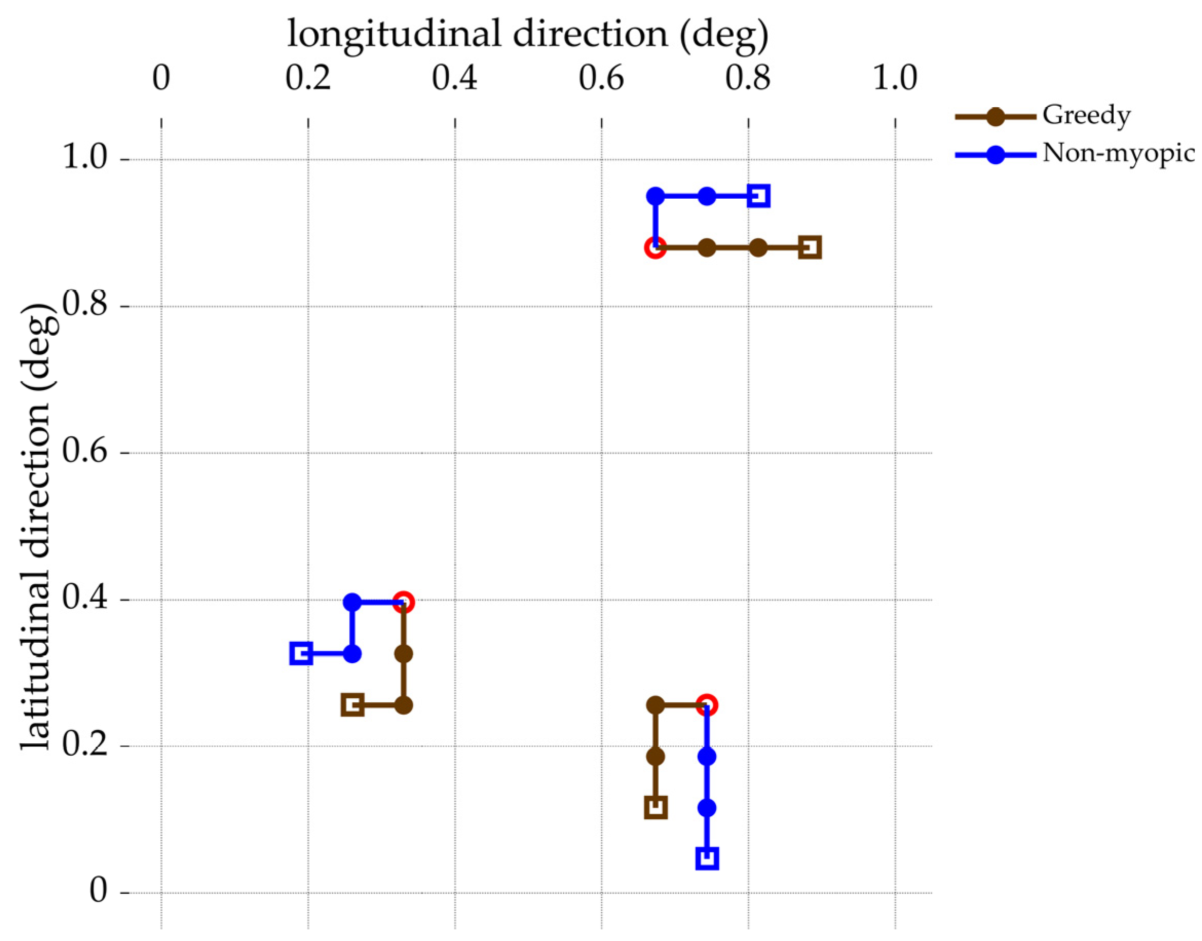
Figure 9 shows the simulation result of the paths of three gliders from a simulation run.
In this simulation, ten simulation runs are performed, each starting from the time
The initial starting locations of the three gliders are randomly set within the operational area. For each run, both the non-myopic optimization and the greedy optimization are performed with the same simulation setup.
Figure 9 also shows the simulation result of the paths of three gliders from a greedy optimization. After each simulation run, the
is calculated for both the cases of optimization considering greedy and non-myopic information gain. The results are presented in
Table 3. Additionally, in the last column of
Table 3, the percentage improvement in
achieved through the non-myopic optimization compared to the greedy optimization is also provided.
Upon analysis of the results, it can be observed that the non-myopic optimization consistently yields higher values compared to the greedy optimization for all ten simulation runs. The improvement percentages range from approximately 9.7% to 15.8%, with an average improvement of around 11.6% across the ten simulation runs. By considering information gains from future time steps, the gliders can better plan their paths and collect more informative data, leading to more accurate flow field predictions at a future targeted time.
The results also validate the effectiveness of the distributed strategy for implementing MCTS, enabling effective decision-making with about of computation time compared to the implementation of the MCTS on a single vehicle. This reduction in computation time is crucial for the real-time decision-making of AMVs. It is worth noting that while the distributed MCTS method has demonstrated promising results in this simulation study, there is great potential for further performance improvement. One area of future research work for the authors is to explore adaptively allocating computational budgets to the subtrees, to further enhance the capability of distributed MCTS in obtaining optimal and reliable decisions.
Overall, the consideration of multiple future time steps, the receding horizon optimization, and the distributed MCTS demonstrate a promising approach to optimize the non-myopic paths of AMVs and achieve more accurate flow field predictions for a targeted time.
6. Conclusions
This research article presents a novel data-driven closed-loop dynamic data-driven application system that effectively addresses the challenge of high-resolution and accurate flow field prediction in ocean environments. The DDDAS leverages a hybrid data-driven flow model for trend prediction, along with a Gaussian process model for residual fitting. The assimilation of spatially correlated flow-sensing data from AMVs using the Kriged ETKF further enhances model online learning and achieves accurate spatiotemporal flow prediction. The proposed receding horizon strategy and distributed strategy of implementing Monte Carlo tree search is demonstrated to be effective in optimizing AMVs’ coordinated flow-sensing paths, enabling non-myopic path planning, and solving large-scale tree searching-based optimization problems in a timely manner. The proposed DDDAS offers a comprehensive and effective solution for achieving high-resolution and accurate flow field prediction in ocean environments using AMV networks.
As future research directions, several potential avenues can be explored. Firstly, investigating the integration of other machine learning models, such as deep neural networks, and data-driven techniques into the DDDAS may lead to further improvements in computational efficiency and prediction accuracy of complex oceanic processes. Additionally, the application of the DDDAS can be extended to incorporate a wider range of ocean data, such as ocean temperature and salinity, to achieve a more comprehensive prediction of ocean environments. Furthermore, optimizing the number of AMVs for environmental sensing is crucial, as it can lead to ocean prediction with the required level of accuracy with a minimum number of AMVs needed. This optimization has the potential to reduce costs and resource requirements for the system, considering the high costs associated with deploying and operating AMVs in ocean environments.

 ,
, 


