
Research on an Underwater Target-Tracking Method Based on Zernike Moment Feature Matching
 , ,
, ,
Abstract
:1. Introduction
2. AUV Target-Tracking System Based on Mechanical Scanning Sonar
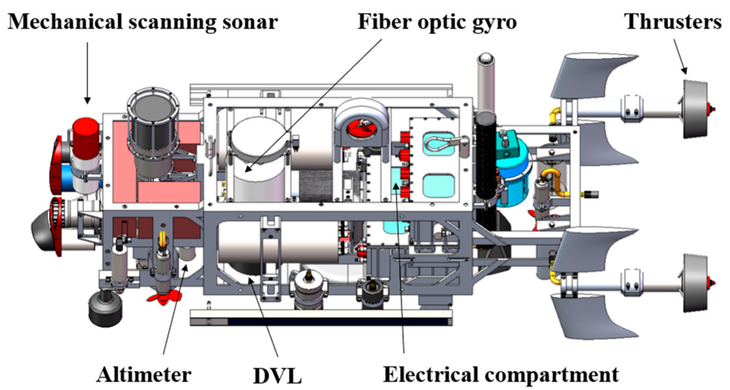
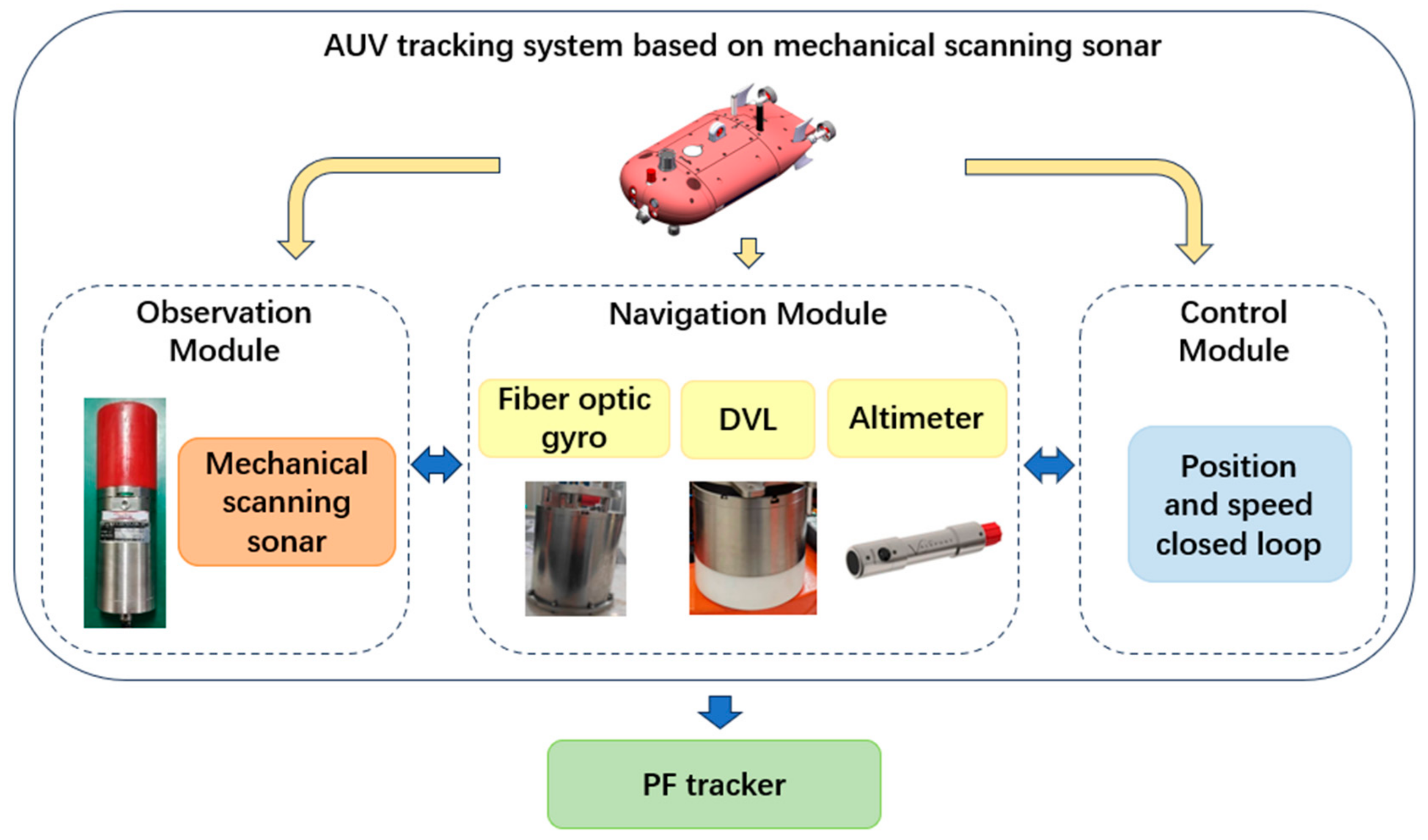
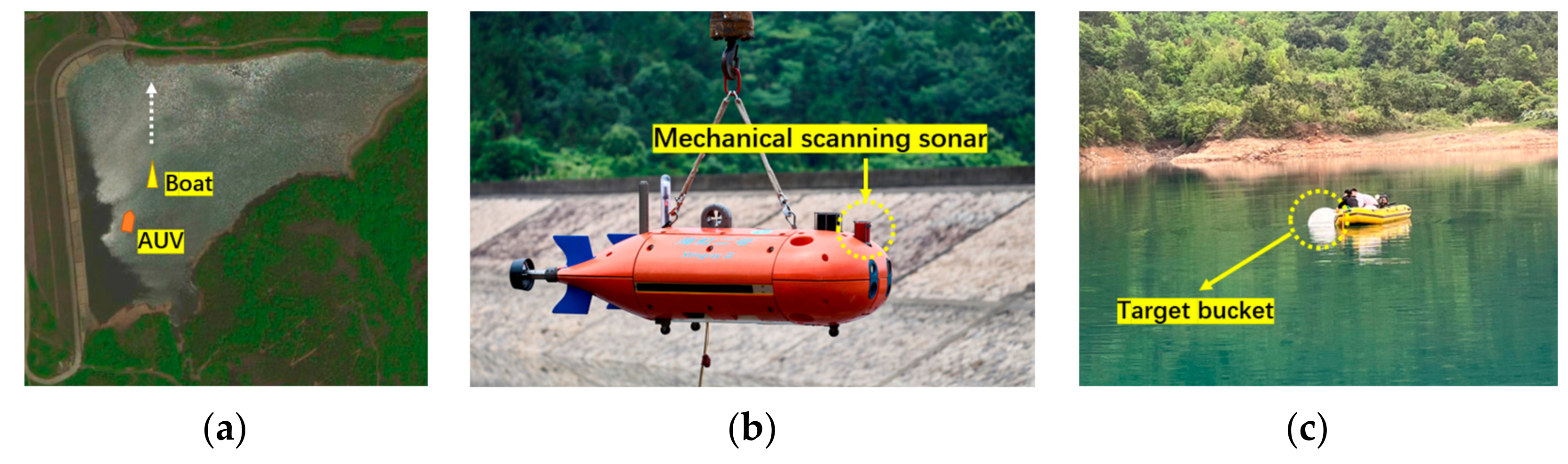
2.1. Hardware Architecture
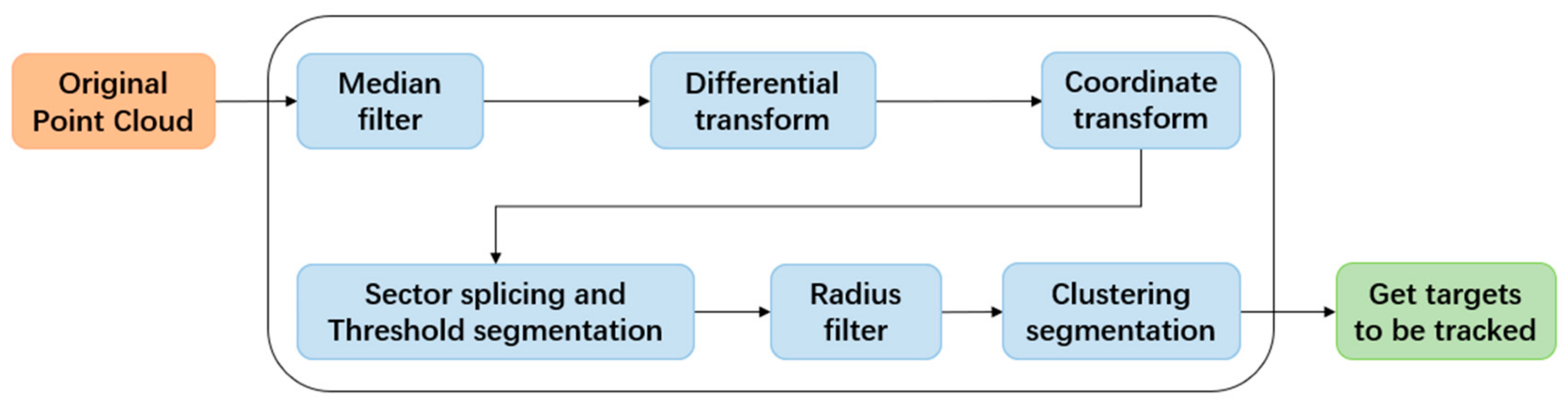
2.2. Mechanical Scanning Sonar Data Preprocessing
2.2.1. Data Preprocessing
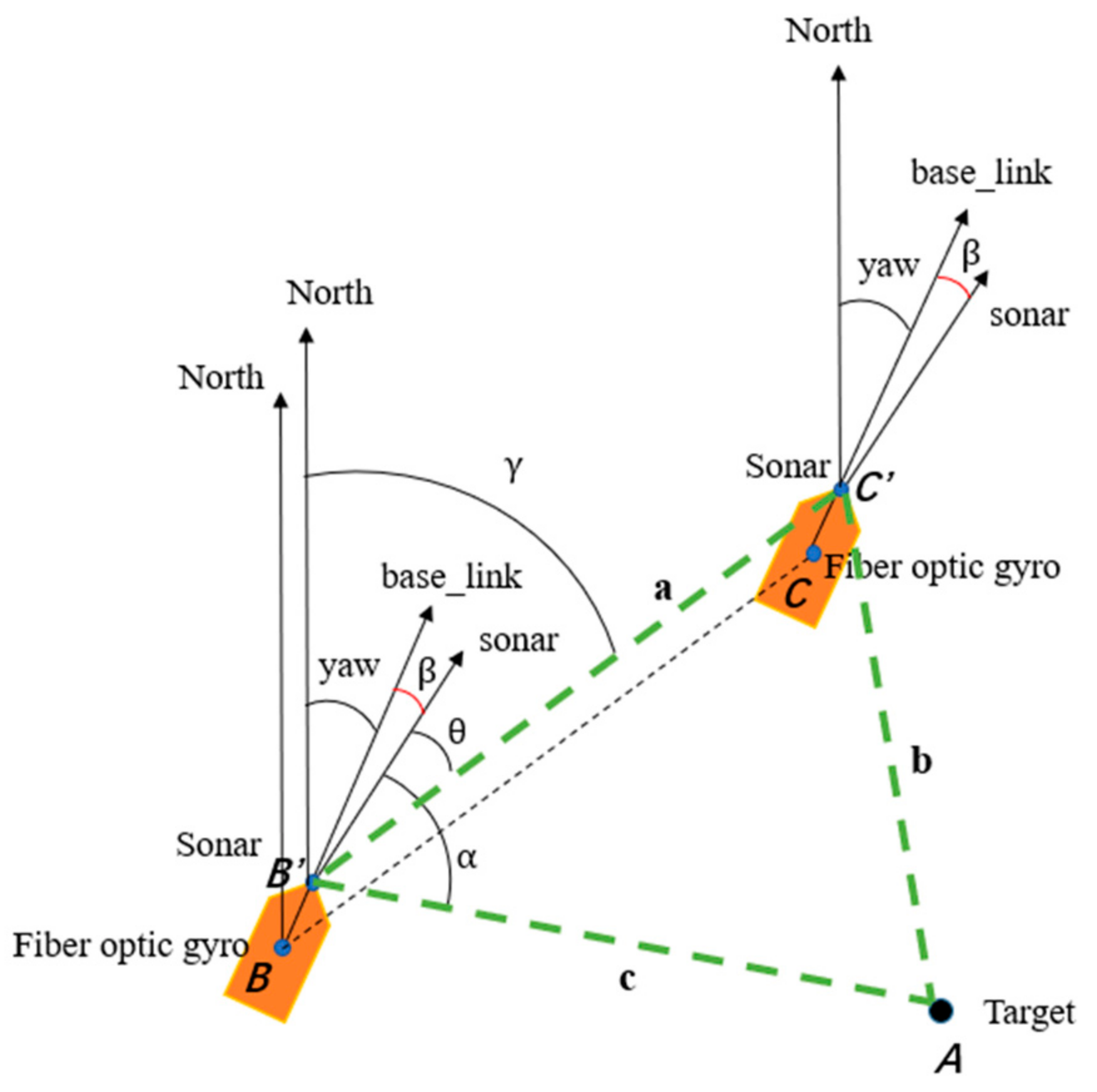
2.2.2. Calibration
- The absolute coordinates and of the AUV at B and C, obtained from GPS;
- The relative coordinates of target A at B and C positions under the sonar coordinate system;
- The yaw angles at B and C.
2.3. Algorithm Design
2.3.1. Feature-Description Vector Construction
2.3.2. Tracking System Initialization
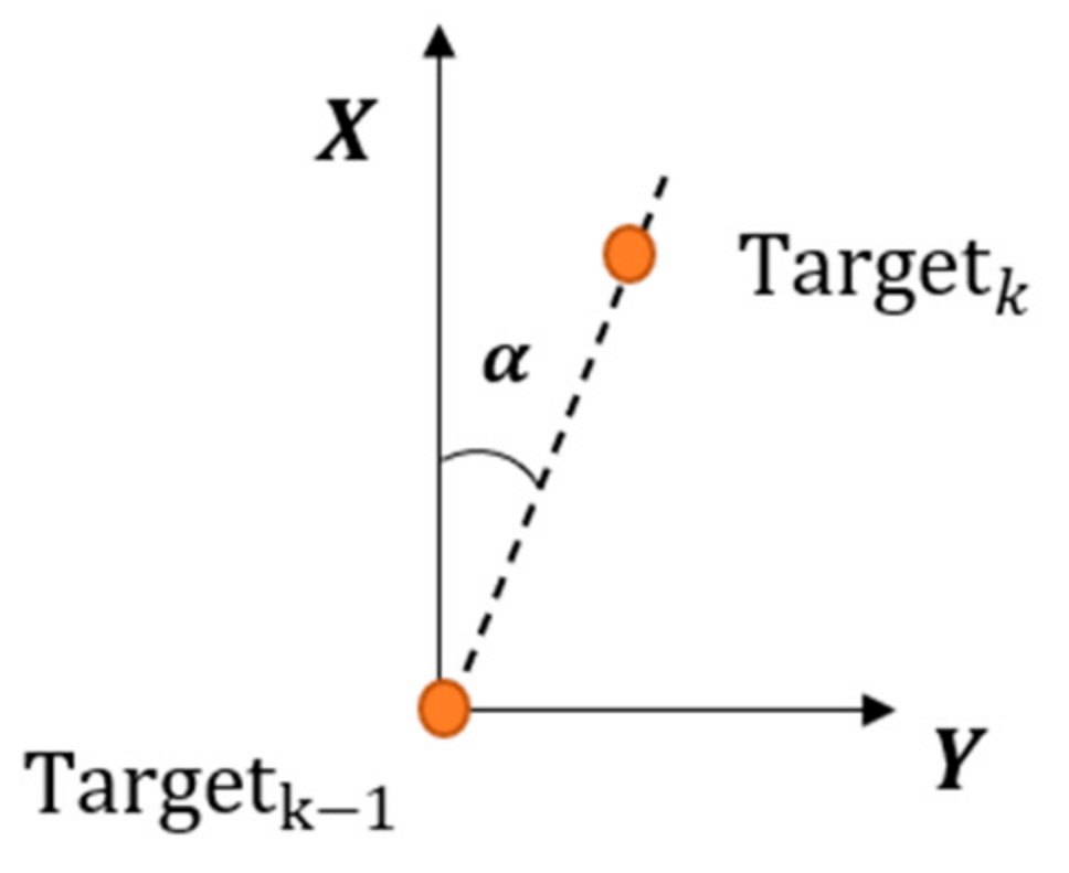
2.3.3. State Transition Model
2.3.4. Observation Model
2.3.5. Resampling
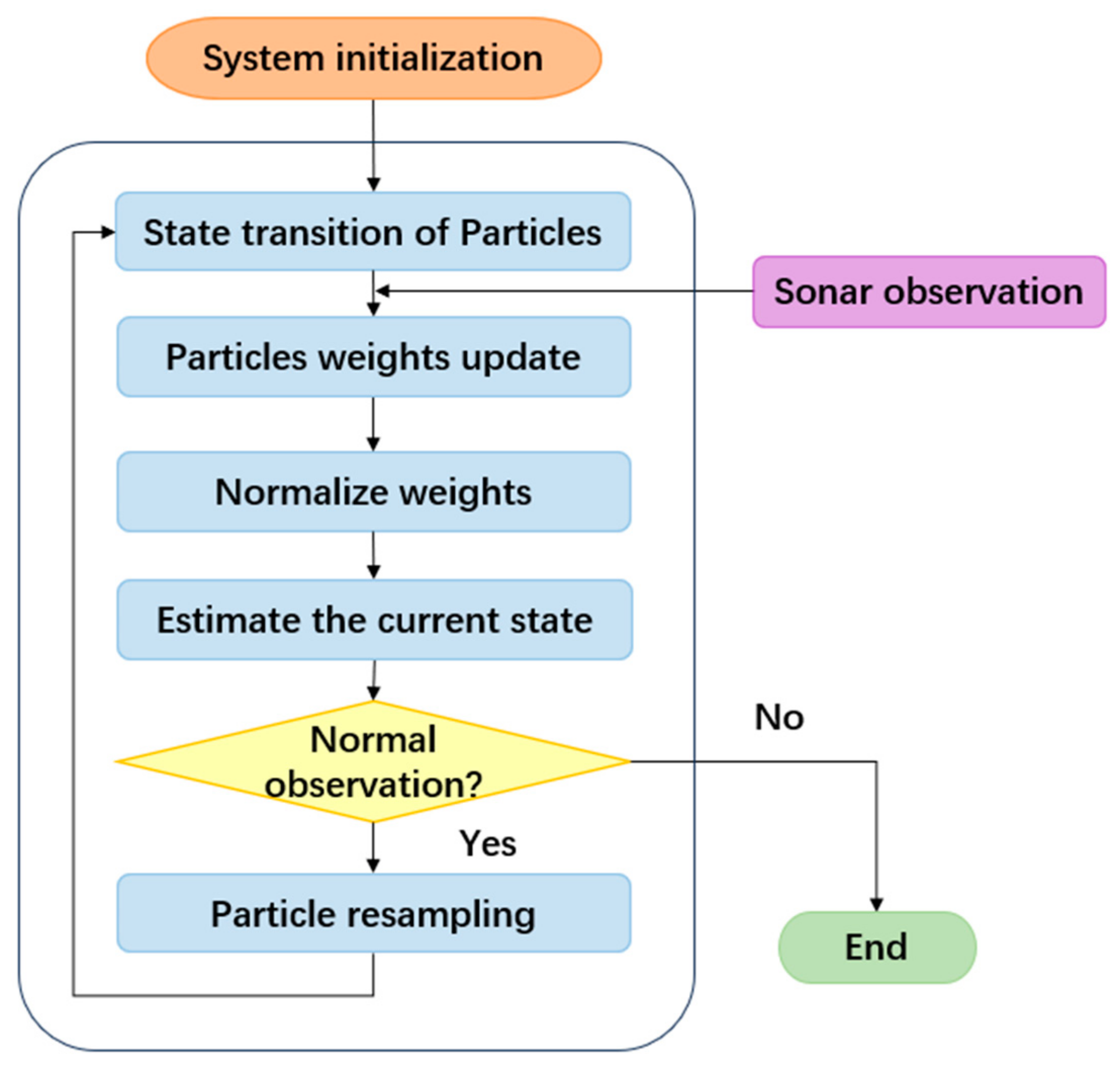
2.3.6. Algorithm
| Algorithm 1: Particle Filter Underwater Target Tracking |
| INPUT: Sonar sequence point clouds |
| OUTPUT: Position estimation of AUV, |
| 1: Initialize feature template, |
| 2: While (Sonar sequence point clouds arrive) do |
| 3: FOR |
| 4: sample |
| 5: |
| 6: |
| 7: END FOR |
| 8: |
| 9: FOR |
| 10: |
| 11: END FOR |
| 12: |
| 13: |
| 14: END WHILE |
3. Experiments and Results
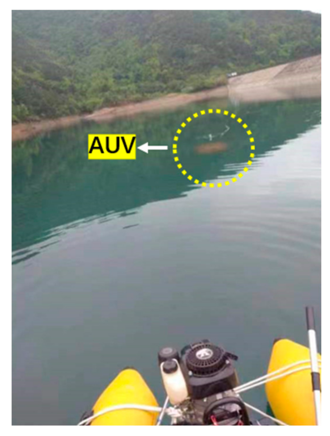
3.1. Experimental Scenes
- Static target with AUV hovering observation;
- Dynamic target with AUV hovering observation;
- Dynamic target with AUV following observation.
3.2. Data Analysis
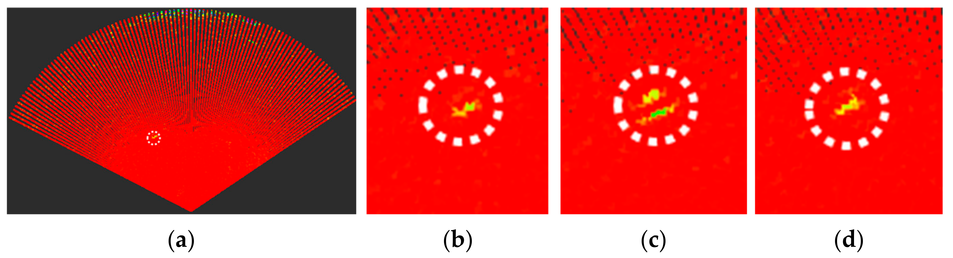
3.2.1. Static Target with AUV Hovering Observation
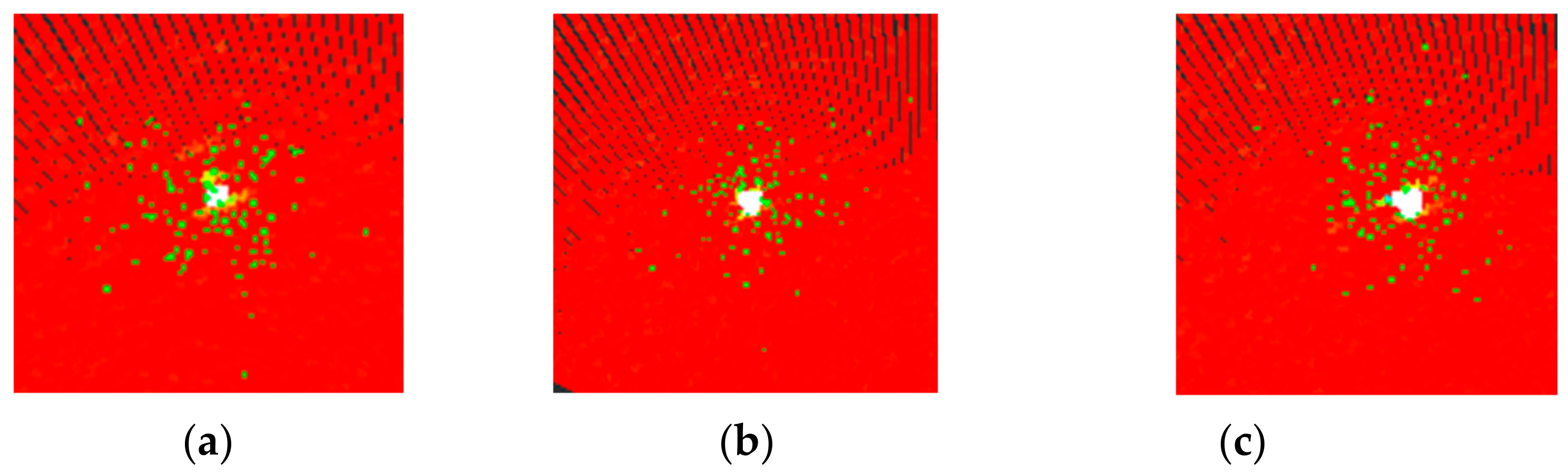
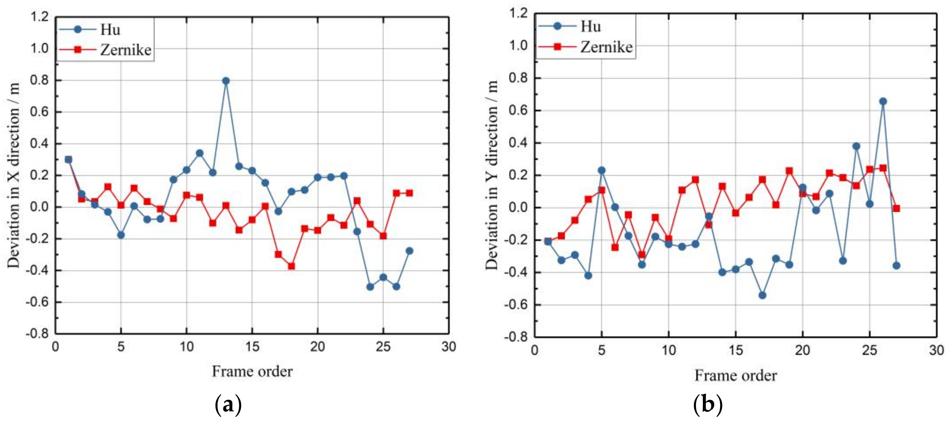
3.2.2. Dynamic Target with AUV Hovering Observation
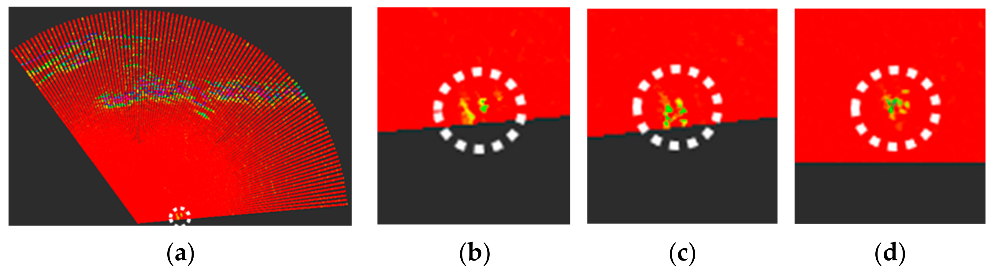
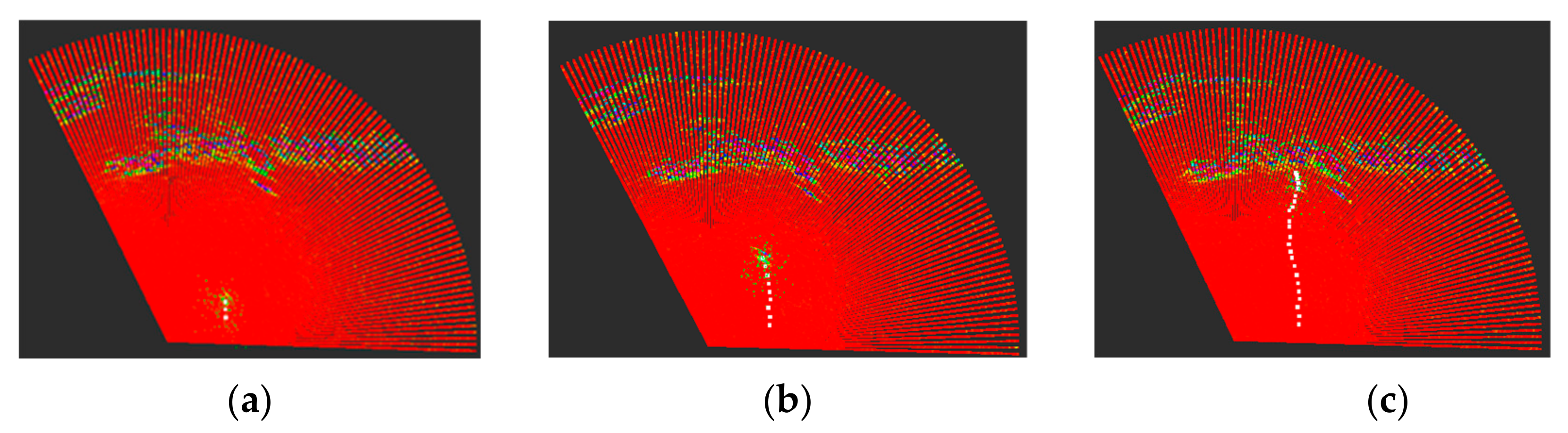
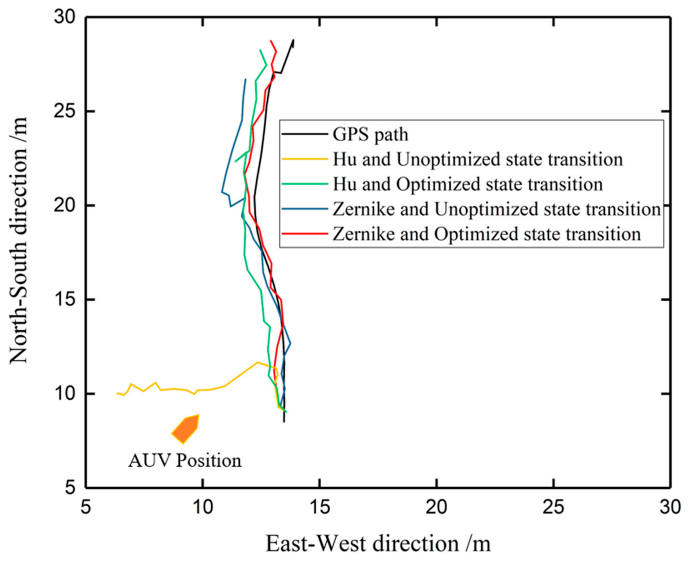
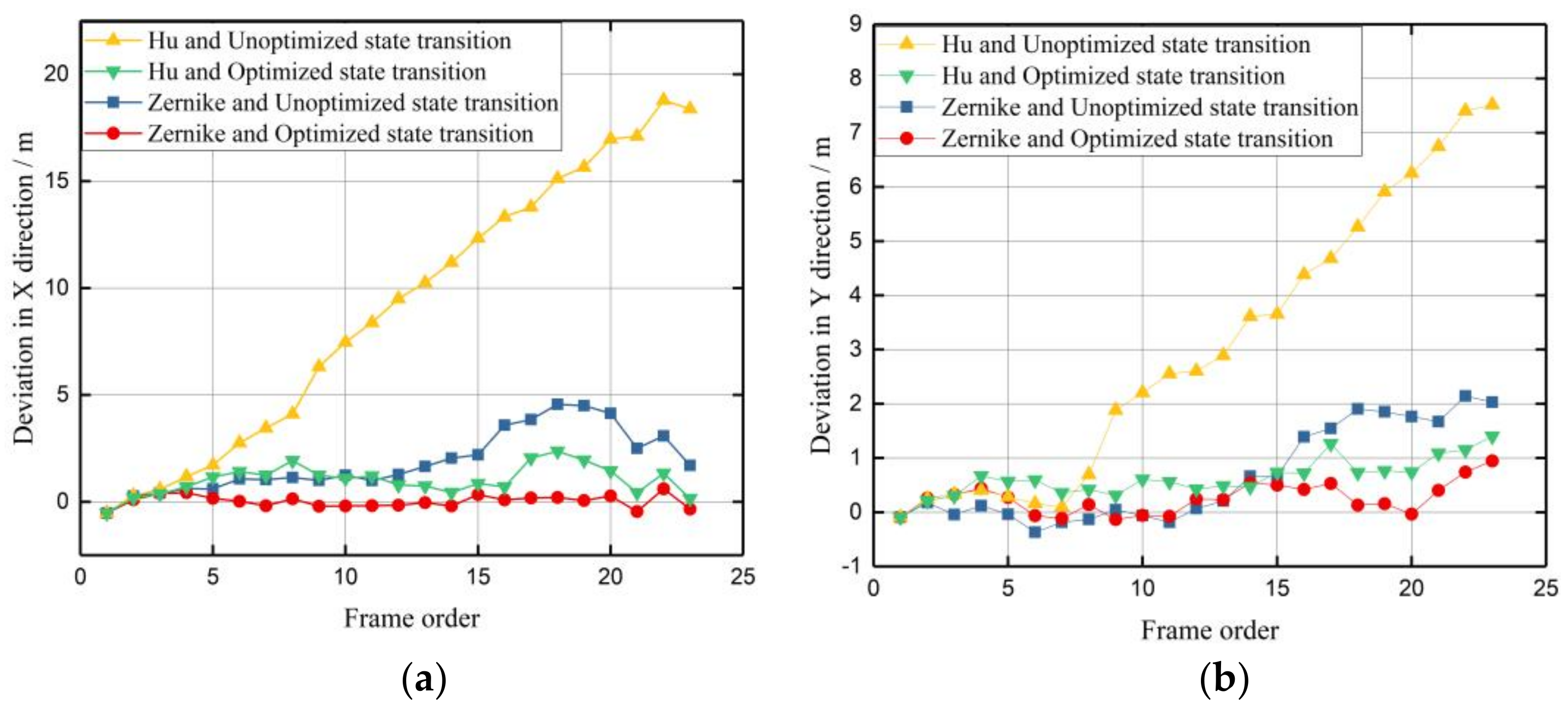
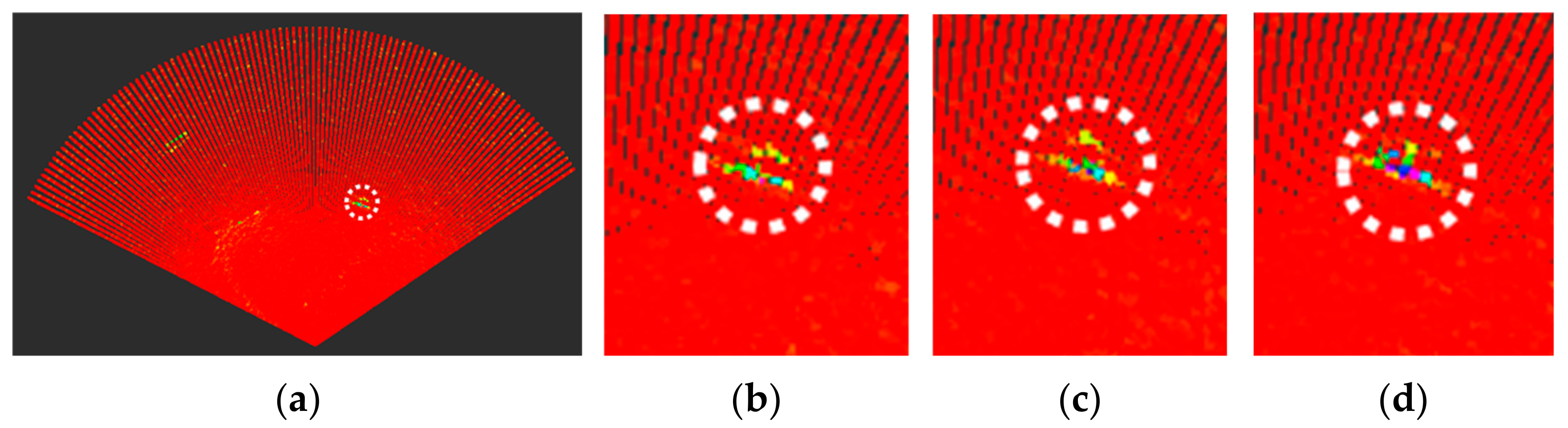
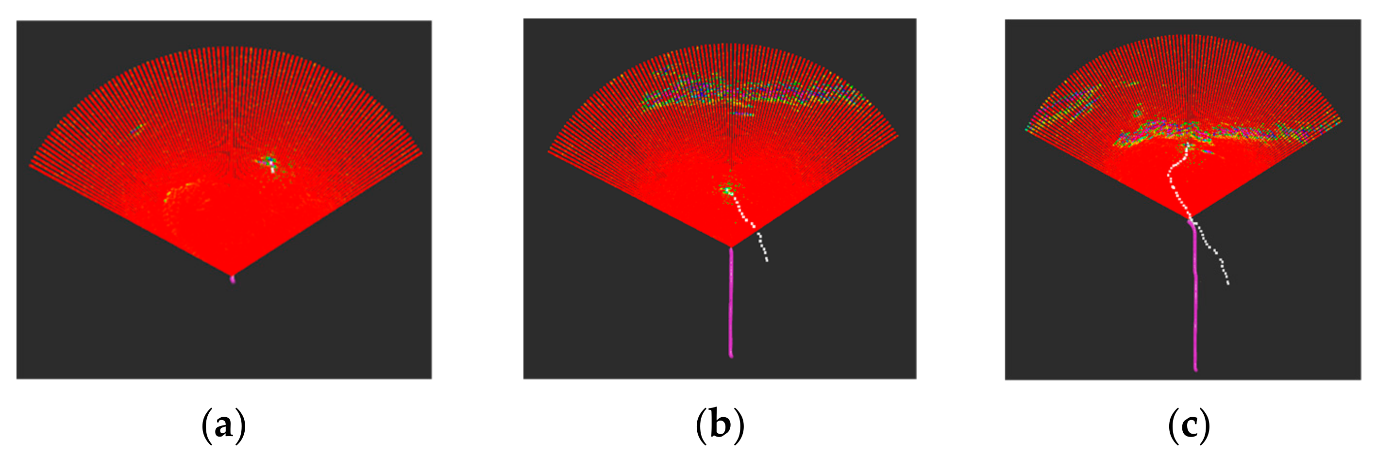
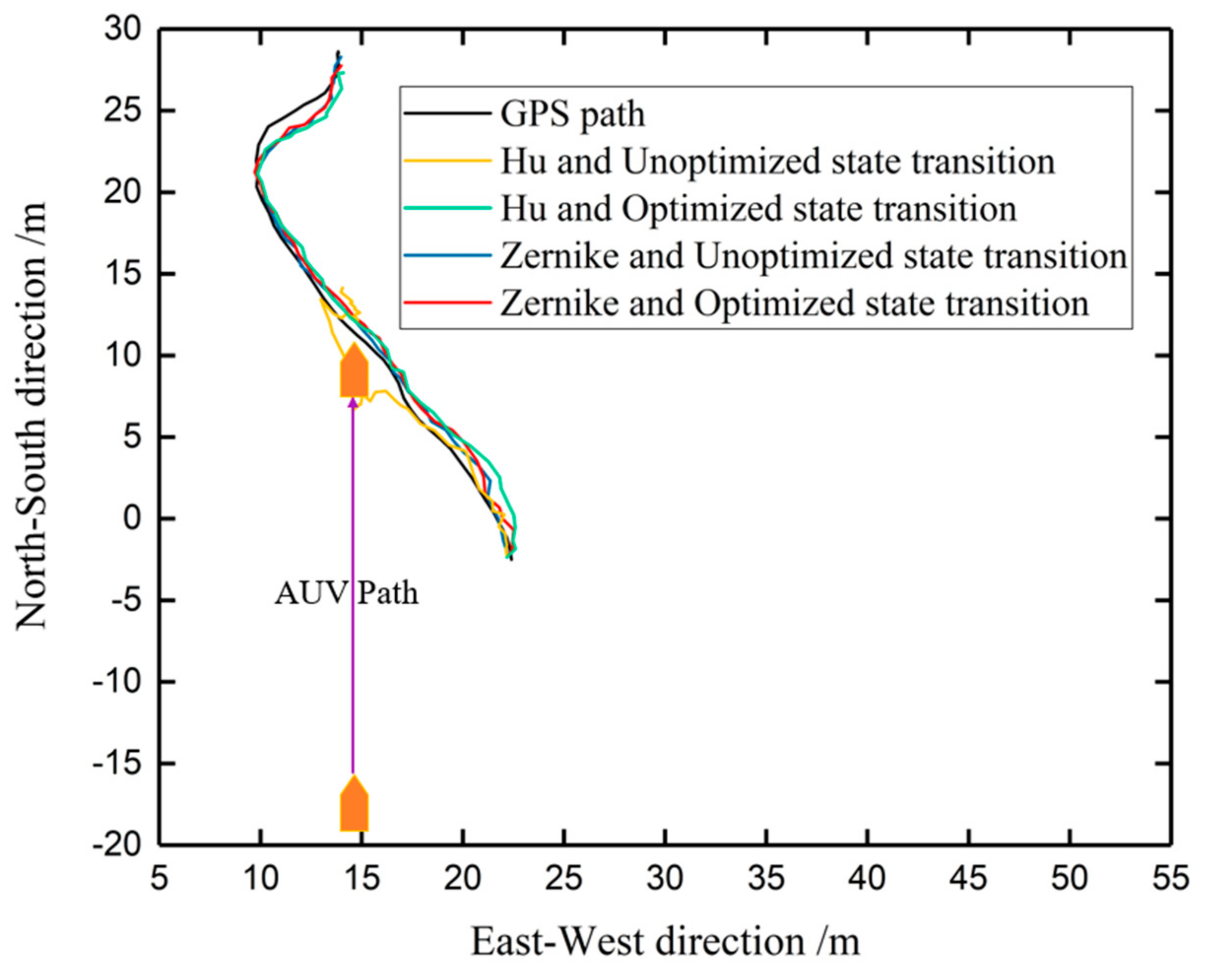
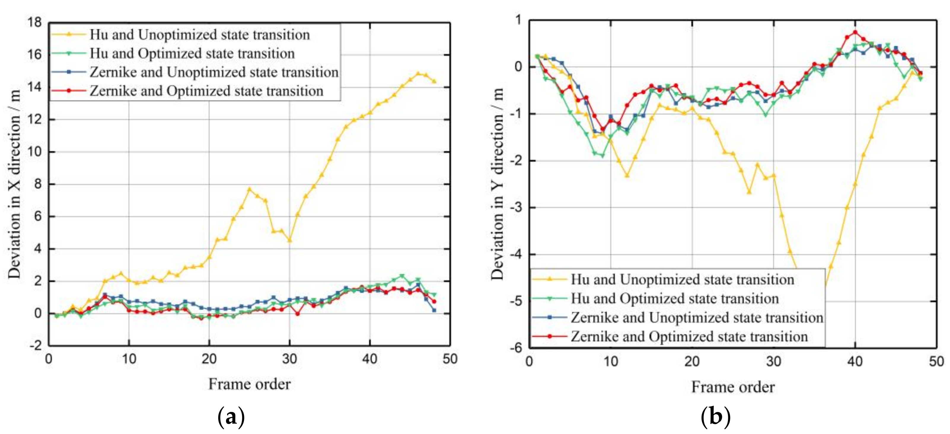
3.2.3. Dynamic Target with AUV following Observation
4. Conclusions
Author Contributions
Funding
Institutional Review Board Statement
Informed Consent Statement
Data Availability Statement
Conflicts of Interest
References
- Barfoot, T.D. State Estimation for Robotics; Gao, X., Xie, X.J., Eds.; Xi’an Jiaotong University Press: Xi’an, China, 2018. [Google Scholar]
- Handschin, J.E. Monte Carlo Techniques for Filtering and Prediction of Nonlinear Stochastic Processes; University of London: London, UK, 1968. [Google Scholar]
- Masmitja, I.; Bouvet, P.J.; Gomariz, S. Underwater mobile target tracking with particle filter using an autonomous vehicle. In Proceedings of the OCEANS, Aberdeen, UK, 19–22 June 2017; pp. 1–5. [Google Scholar]
- Tan, P.L.; Wu, X.B.; Zhang, X.Y. Review on Underwater Target Recognition Based on Sonar Image. Digit. Ocean. Underw. Warf. 2022, 5, 342–353. [Google Scholar]
- Ma, S. Multi-Target Tracking of AUV Based on Forward Looking Sonar; Harbin Engineering University: Harbin, China, 2016. [Google Scholar]
- Nguyen, H.T.; Lee, E.; Bae, C.H. Multiple object detection based on clustering and deep learning methods. Sensors 2020, 20, 4424. [Google Scholar] [CrossRef] [PubMed]
- Li, Q.W.; Huo, G.Y.; Zhou, Y. Sonar Image Processing; Science Press: Beijing, China, 2015. [Google Scholar]
- Gong, W.J.; Tian, J. Underwater sonar image small target recognition method based on shape features. J. Appl. Acoust. 2021, 40, 294–302. [Google Scholar]
- Huang, S.W.; Zhu, Z.T. A sonar image target tracking algorithm based on particle filter. Ship Sci. Technol. 2019, 41, 135–139. [Google Scholar]
- Wang, X.; Zou, Z.W. Target Detection in Colorful Imaging Sonar Based on Multi-feature Fusion. Comput. Sci. 2019, 46, 177–181. [Google Scholar]
- Zan, M.E.; Zhou, H. Survey of Particle Filter Target Tracking Algorithms. Comput. Eng. Appl. 2019, 55, 8–17. [Google Scholar]
- Liu, T.J. Adaptive hierarchical particle filter in dynamic tracking scenarios. J. Electron. Compon. Inf. Technol. 2018, 1, 17–21. [Google Scholar]
- Zhang, T.D.; Wan, L. Underwater Object Tracking Based on Improved Particle Filter. J. Shanghai Jiaotong Univ. 2012, 46, 943–948. [Google Scholar]
- Wang, Z.Q. Algorithm Research and System Implementation of Underwater Target Detection and Tracking Based on Forward-Looking Sonar; Harbin Engineering University: Harbin, China, 2019. [Google Scholar]
- Li, J. Research on Target Detection and Tracking of Forward-Looking Sonar; Harbin Engineering University: Harbin, China, 2019. [Google Scholar]
- Li, H.G. Study on Moment Technique Applications in Underwater Acoustic Image Classification and Recognition; Dalian University of Technology: Dalian, China, 2018. [Google Scholar]
- Kim, W.Y.; Kim, Y.S. A region-based shape descriptor using Zernike moments. Signal Process Image Commun. 2020, 16, 95–102. [Google Scholar] [CrossRef]
- Hu, M.K. Visual pattern recognition by moment invariants. IRE Trans. Inf. Theory 1962, 8, 179–187. [Google Scholar]
- Teague, M.R. Image analysis via the general theory of moments. J. Opt. Soc. Am. 1980, 70, 1468. [Google Scholar] [CrossRef]
- Mukundan, R.; Ramakrishnan, K.R. Fast computation of Legendre and Zernike moments. Pattern Recogn. 1995, 28, 1433–1442. [Google Scholar] [CrossRef]
- Carpenter, J.; Clifford, P.; Fearnhead, P. Improved particle filter for non-linear problems. IEE Proc.-Radar Sonar Navig. 1999, 146, 2–7. [Google Scholar] [CrossRef]
- Wang, F. Particle filters for visual tracking. Commun. Comput. Inf. Sci. 2011, 152, 107–112. [Google Scholar]
- Mikami, D.; Otsuka, K.; Yamato, J. Memory-based particle filter for tracking objects with large variation in pose and appearance. In Proceedings of the European Conference on Computer Vision, Heraklion, Greece, 5–11 September 2010; pp. 215–228. [Google Scholar]


| 1 | 3 | 3 | 5 | 3 | 5 | 7 | |
| 3 | 5 | 7 | 7 | 9 | 9 | 9 |
| Parameter | Value |
|---|---|
| Frequency | 675 kHz |
| Pulse length | 110 s |
| Start gain | 10 dB |
| Range | 40 m |
| Step size | 1.2° |
| Sector width | 120° |
| Template Features Moments | Hu | Zernike |
|---|---|---|
| 1.8182 | 1.3843 | |
| 5.4463 | 3.9044 | |
| 6.4658 | 7.1292 | |
| 8.7426 | 10.1156 | |
| 16.5203 | 12.8892 | |
| 12.0946 | 16.6743 | |
| 16.6599 | 20.3906 |
| Deviation | Hu | Zernike |
|---|---|---|
| X deviation mean/m | 0.0492 | −0.0291 |
| X deviation variance/m2 | 0.0754 | 0.0187 |
| Y deviation mean/m | −0.1559 | 0.0292 |
| Y deviation variance/m2 | 0.0711 | 0.0238 |
| S/m | 0.3791 | 0.1883 |
| Template Features Moments | Hu | Zernike |
|---|---|---|
| 2.5634 | 0.1720 | |
| 7.7801 | 3.0683 | |
| 9.5124 | 5.9074 | |
| 10.2396 | 9.5158 | |
| 21.8039 | 12.3790 | |
| 14.9056 | 15.5995 | |
| 20.2795 | 19.2436 |
| Deviation | Hu Non-Optimized | Hu Optimized | Zernike Non-Optimized | Zernike Optimized |
|---|---|---|---|---|
| X deviation mean/m | 9.0516 | 1.0108 | 1.8659 | 0.0221 |
| X deviation variance/m2 | 39.5647 | 0.4556 | 1.9981 | 0.0798 |
| Y deviation mean/m | 3.0310 | 0.6296 | 0.6589 | 0.2486 |
| Y deviation variance/m2 | 6.3450 | 0.1157 | 0.7506 | 0.0807 |
| S/m | 9.6144 | 1.2914 | 2.0941 | 0.4059 |
| Template Features Moments | Hu | Zernike |
|---|---|---|
| 2.5622 | 0.1983 | |
| 7.0985 | 2.7418 | |
| 8.6391 | 5.9358 | |
| 9.3487 | 9.1654 | |
| 18.3708 | 12.9062 | |
| 13.3045 | 15.3804 | |
| 19.2669 | 18.5920 |
| Deviation | Hu Non-Optimized | Hu Optimized | Zernike Non-Optimized | Zernike Optimized |
|---|---|---|---|---|
| X deviation mean/m | 6.3420 | 0.6765 | 0.7829 | 0.5286 |
| X deviation variance/m2 | 22.7151 | 0.4830 | 0.2180 | 0.3365 |
| Y deviation mean/m | −1.7531 | −0.4954 | −0.3845 | −0.3170 |
| Y deviation variance/m2 | 1.7965 | 0.3502 | 0.2768 | 0.2386 |
| S/m | 6.7260 | 1.1086 | 1.0502 | 0.8761 |
Disclaimer/Publisher’s Note: The statements, opinions and data contained in all publications are solely those of the individual author(s) and contributor(s) and not of MDPI and/or the editor(s). MDPI and/or the editor(s) disclaim responsibility for any injury to people or property resulting from any ideas, methods, instructions or products referred to in the content. |
© 2023 by the authors. Licensee MDPI, Basel, Switzerland. This article is an open access article distributed under the terms and conditions of the Creative Commons Attribution (CC BY) license (https://creativecommons.org/licenses/by/4.0/).
Share and Cite
Gao, W.; Zhou, S.; Liu, S.; Wang, T.; Zhang, B.; Xia, T.; Cai, Y.; Leng, J. Research on an Underwater Target-Tracking Method Based on Zernike Moment Feature Matching. J. Mar. Sci. Eng. 2023, 11, 1594. https://doi.org/10.3390/jmse11081594
Gao W, Zhou S, Liu S, Wang T, Zhang B, Xia T, Cai Y, Leng J. Research on an Underwater Target-Tracking Method Based on Zernike Moment Feature Matching. Journal of Marine Science and Engineering. 2023; 11(8):1594. https://doi.org/10.3390/jmse11081594
Chicago/Turabian StyleGao, Wenhan, Shanmin Zhou, Shuo Liu, Tao Wang, Bingbing Zhang, Tian Xia, Yong Cai, and Jianxing Leng. 2023. "Research on an Underwater Target-Tracking Method Based on Zernike Moment Feature Matching" Journal of Marine Science and Engineering 11, no. 8: 1594. https://doi.org/10.3390/jmse11081594