Investigation of Submergence Depth and Wave-Induced Effects on the Performance of a Fully Passive Energy Harvesting Flapping Foil Operating Beneath the Free Surface

Abstract

This paper investigates the performance of a fully passive flapping foil device for energy harvesting in a free surface flow. The study uses numerical simulations to examine the effects of varying submergence depths and the impact of monochromatic waves on the foil’s performance. For the numerical simulations, a in-house artificial compressibility two-phase solver is employed and coupled with a rigid body dynamic solver. The results show that the fully passive flapping foil device can achieve high efficiency for submergence depths between 4 and 9 chords, with an “optimum” submergence depth where the flapping foil performance is maximised. The effects of regular waves on the foil’s performance were also investigated, showing that waves with a frequency close to that of the natural frequency of the flapping foil-aided energy harvesting. Overall, this study provides insights that could be useful for future design improvements for fully passive flapping foil devices for energy harvesting operating near the free surface.

1. Introduction

The technology for flapping foils was inspired by fish locomotion. Evolution through hundreds of millions of years has enabled fish to develop highly efficient thrusting mechanical systems [1]. Except from thrust production, these devices can also be used to capture energy from water currents, such as tidal currents or from rivers. When the pitching amplitude is higher than a threshold value, for a given frequency and heave amplitude, called the feathering limit, the foil switches from the thrust production mode to the energy harvesting mode [2]. Their main competitors are horizontal axis turbines and vertical axis turbines. Compared to these types of turbines, flapping foils have certain benefits. Firstly, the efficiency of flapping foils remains high even in very large angles of attack with the flow, due to the phenomenon of dynamic stalling which insures that lift remains temporarily high [3]. This also means that oscillating hydrofoils can harvest energy from a wider range of current velocities [4] compared to conventional turbines with a specific design point. The device is also more robust, as centrifugal stresses are absent, and more environmentally friendly, as blade tip velocities are lower [5,6]. Finally, their rectangular sweeping profiles are perfect for shallow and wide fluid channels.

Energy harvesting foils were first proposed by McKinney and DeLaurier in 1981 [7]. It has been shown that flapping foils can offer high performance for both the production of thrust or energy harvest. Many studies have taken place, either experimental [8,9] or numerical (a collection can be found here in [4]), showing the applicability of these devices and highlighting their advantages and disadvantages over conventional devices. Incorporating chord-wise flexibility also seems promising as increases in performance are significant, as shown in [10]. Importantly, this device can be simplified by attaching the heaving degree of freedom (DOF) to a spring and damper, and imposing the motion of the pitching DOF, creating the semi-passive flapping foil [11]. The pitching motion creates a variable lift force that makes the foil oscillate in its heaving DOF. Alternatively, both heaving and pitching DOFs can be attached to springs and dampers, creating the fully passive flapping foil, which oscillates without external forcing (not even initially) when it faces fluid flow. By suitably tuning the structural parameters, a periodical, high-energy content motion, in the heaving DOF can be sustained. The authors of [12] explored the modes that are achievable by different choices of structural parameters. These fully passive flapping foils proved to be a viable alternative to the active or semi-passive flapping foils that require intricate mechanisms to enforce the movement. These extra mechanisms raise the risk of failure, the construction cost, and the cost of maintenance. They also have additional power losses. Most research in the past has shown that the fully passive foil exhibits a lower performance compared to the active ones. Recent numerical experiments, however, by [13], aiming to optimize the device by exploring the available domain of the structural parameters showed that the fully passive flapping foil can perform as well as active flapping foils while maintaining a much simpler structure. In addition, it was shown that good performance is available for a wide range of parameters, which is necessary for a practical application.

While a plethora of research has been conducted for active energy harvesting flapping foils under more realistic conditions, not so much has been conducted for fully passive flapping foils. The effects of flow perturbation by other flapping foils upstream in [14]. Additionally, in [15], feedback control was added to the flapping foil system, leading to operation of the system in the dynamic stall regime.

However, there is a lack of research on the influence of the free surface, which is important if we want a more realistic assessment of the device as flapping foils will likely be placed close to it, for example, due to the need to operate in shallow waters, either in rivers or relatively close to shores. The effects of proximity to the free surface, for instance, or the effects of waves, have not yet been explored. The effects of the free surface on active flapping foils were studied by [16,17], whose results were similar, finding that the effect of the free surface on the performance of the devices was mostly negative, but becomes quickly irrelevant as submergence depth increases.

With regards to the influence of a wavy free surface on flapping foils, most research has focused so far on thrust producing flapping foils. In [18], they were the first to propose that a flapping foil on the bow of a ship could convert wave power into propulsive power and proved this case. The effect of regular waves on thrust producing flapping foils, both rigid and flexible, has been studied in [19], where it was found that power output is significantly increased, especially when the frequency of the waves matches that of the foil and the phase difference is suitable. Efficiency was higher when a flexible foil was used, but was not affected that greatly, in general. An investigation into 3D effects and free surface wave patterns was carried out by [20]. In [21], they studied thrust producing flapping foils in waves, for constant submergence depth and wave heights using a boundary element method. It was found that an increase in wave frequency increased the power output but decreased the efficiency. It is distinctive that the amplitudes of the motion fluctuated periodically when the frequencies of the foil and waves did not match. When the frequencies did match there were no fluctuations, as the phase difference of foil and wave remains constant throughout the periods, but the phase difference played a significant role. In [22] they studied a semi-active flapping foil operating in waves and currents, in a shear flow with variable bathymetry (simulating nearshore conditions) using Boundary Element Method (BEM) analysis. For a specific moderate wave frequency, significant efficiency can be achieved both when the foil and wave frequency match or do not by operating at appropriate pitch angles. Peak efficiency was achieved, however, even for small pitching angles when the foil matched the frequency of the waves or was double that, and the phase difference was suitable for each case.

This work is a continuation of the work in [23], in which the authors studied how shear presence in the flow affects the fully passive flapping foil device, and began the examination of the influence of the free surface. Particularly, the influence of a calm free surface is studied in depth, for a broad range of submergence depths and multiple Froude numbers. An initial step in the examination of the impact of monochromatic waves is also taken, examining cases when the wave frequency is close to the flapping foil’s or when the wavelength is comparable to the chord length of the foil.

This paper is structured as follows: In Section 2, the in-house Computational Fluid Dynamics solver MaPFlow used for the numerical analysis is outlined briefly. Its strong coupling to a Rigid Body Dynamics solver to simulate the dynamics problem is also detailed. In Section 3, the physical problem is explained and the numerical setup of the solver is given. In Section 4, the effect of submergence depth is explored for various Froude numbers. Finally, the passive foil is investigated operating under monochromatic waves of different frequencies and their effect on the foil performance is presented.

2. Numerical Methodology

Fluid Structure Interaction (FSI) problems are numerically investigated by combining two separate computational algorithms. Firstly, a flow solver is utilised to describe the fluid motion, and secondly a dynamic solver that computes the structure’s response under the flow excitation. The flapping foil is considered submerged and thus the presence of the free surface requires the solution of a two-phase problem. This methodology is implemented as part of the CFD code MaPFlow. The in-house code is developed in NTUA [24,25], and has proven capable of handling both compressible and purely incompressible flows on arbitrary polyhedral meshes. The code is able to perform in a multi-processing environment utilising the Message Parsing Interface (MPI) protocol, while the grid partitioning is performed using the Metis Library [26]. The numerical methodology is outlined in this section.

2.1. Governing Equations

Two-phase incompressible flows are solved using the artificial compressibility method (ACM) [27], coupled with the Volume of Fluid (VoF) approach [28]. The ACM solves the unsteady system of equations by utilizing the dual-time stepping technique [29], where at each real time iteration a pseudo–steady state problem is solved. This is accomplished by augmenting the original unsteady system of equations by pseudo–time derivatives of the unknown variables. Convergence is accomplished once these derivatives approach zero and thus the original system of equations is obtained. The ACM assumes a relation between the pressure and the density field during pseudo time. The blending is performed by introducing a numerical parameter $\beta$, that is, $\frac{\partial \rho }{\partial p}{|}_{\tau }=\frac{1}{\beta }$. This free parameter for typical free surface flows takes values between 5 and 10 ([30,31]). The governing system of equations is described by Equation (1).

$$\Gamma \frac{\partial }{\partial \tau }{\int }_{D_i}\overrightarrow{Q}\mathrm{d}D+{\Gamma }_e\frac{\partial }{\partial t}{\int }_{D_i}\overrightarrow{Q}\mathrm{d}D+{\int }_{\partial D_i}\left({\overrightarrow{F}}_c-{\overrightarrow{F}}_v\right)\mathrm{d}S={\int }_{D_i}{\overrightarrow{S}}_q\mathrm{d}D$$

(1)

The above system of equations expresses the change of the primitive variables $\overrightarrow{Q}$ inside a control volume $D_i$ with boundary $\partial D_i$, in time t. The vector $\overrightarrow{Q}={[p,\overrightarrow{\upsilon },\overrightarrow{{\alpha }_l}]}^T$ includes the pressure p, the three-dimensional velocity vector $\overrightarrow{\upsilon }$, and the volume fraction ${\alpha }_l$. The volume fraction ${\alpha }_l$ indicates the presence of either the liquid phase with density ${\rho }_l$, or the presence of the gaseous phase with density ${\rho }_g$. Using the volume fraction, the density of the mixture can be found as ${\rho }_m={\alpha }_l{\rho }_l+(1-{\alpha }_l){\rho }_g$.

Although the system of equations is casted in primitive form, in order to advance the solution in time, the conservative form of the equations is used. The variable transformation between the primitive variables $\overrightarrow{Q}$ and the conservative variables $U={[0,{\rho }_m\overrightarrow{\upsilon },{\alpha }_l]}^T$, is performed using the transformation matrix ${\Gamma }_e$, which is given in Equation (2).

Applying the standard ACM to multi-phase flows, especially when large density ratios are accounted, the system of equations becomes poorly conditioned [32]. This happens because the eigenvalues of the system scale with local density of the flow. In order to alleviate this behaviour, the preconditioning matrix $\Gamma$ of Kunz [33] is used to re-scale the fictitious time derivatives and allow for the efficient time marching of the solution.

$$\Gamma =\left[\begin{array}{ccc}\frac{1}{\beta {\rho }_m}& 0& 0\\ 0& {\rho }_m{I}_{3\times 3}& \overrightarrow{\upsilon }\Delta \rho \\ \frac{{\alpha }_l}{\beta {\rho }_m}& 0& 1\end{array}\right],{\Gamma }_e=\left[\begin{array}{ccc}0& 0& 0\\ 0& {\rho }_m{I}_{3\times 3}& \overrightarrow{\upsilon }\Delta \rho \\ 0& 0& 1\end{array}\right]$$

(2)

In Equation (2), $\Delta \rho$ is the difference between the densities of the liquid and the gas, $\Delta \rho ={\rho }_l-{\rho }_g$, and $I_{3\times 3}$ is the three by three identity matrix.

The surface term of the integral equation includes the convective fluxes ${\overrightarrow{F}}_c$ and the viscous fluxes ${\overrightarrow{F}}_v$. Both vectors are presented in Equation (3). In this Equation, $V_n=\overrightarrow{\upsilon }·\overrightarrow{n}$ is the fluid velocity projected onto the surface normal $\overrightarrow{n}=(n_x,n_y,n_z)$ and $\Delta V$ is the difference between the velocity $V_n$ and the projected grid velocity $V_g={\overrightarrow{\upsilon }}_{vol}·\overrightarrow{n}$.

$${\overrightarrow{F}}_c=\left[\begin{array}{c}{V}_n\\ {\rho }_{m}u\Delta V+p{n}_x\\ {\rho }_{m}v\Delta V+p{n}_y\\ {\rho }_{m}w\Delta V+p{n}_z\\ {\alpha }_l\Delta V\end{array}\right],{\overrightarrow{F}}_v=\left[\begin{array}{c}0\\ {\tau }_{xx}{n}_x+{\tau }_{xy}{n}_y+{\tau }_{xz}{n}_z\\ {\tau }_{yx}{n}_x+{\tau }_{yy}{n}_y+{\tau }_{yz}{n}_z\\ {\tau }_{zx}{n}_x+{\tau }_{zy}{n}_y+{\tau }_{zz}{n}_z\\ 0\end{array}\right]$$

(3)

The viscous stresses ${\tau }_{ij}$, using the Boussinesq approximation are computed as

$${\tau }_{ij}=\left({\mu }_m+{\mu }_t\right)\left(\frac{\partial u_i}{\partial x_j}+\frac{\partial u_j}{\partial x_i}\right)-\frac{2}{3}{\rho }_m{\delta }_{ij}k$$

(4)

where ${\mu }_m$ is the viscosity of the mixture, ${\mu }_t$ is the turbulence viscosity, k is the turbulent kinetic energy and ${\delta }_{ij}$ is the Kronecker’s symbol.

For the turbulence closure, the k-$\omega$ SST model of Menter is employed [34]. In case of free surface flows, it has been noted that the turbulence models tend to overproduce turbulence viscosity in the vicinity of the free surface [35,36]. In order to suppress the turbulent viscosity near the free surface, Devolder et al. [37] introduced a source term in the equation of the turbulent kinetic energy. This source term is activated near the free surface and scales with the local viscosity and the gravity vector.

In order to perform simulations of numerical wave tanks, the lateral boundaries of the domain are equipped with damping zones that absorb any outgoing perturbation and make sure that no reflections occur due to the boundary conditions. In MaPFlow, this is performed by defining forcing zones near the boundaries of the computational domain. Forcing zone technique drives the numerical field to the desired solution by adding source terms to the governing equations. In MaPFlow, source terms are added only to the momentum equations. The form of the source terms is presented in Equation (5). The damping is performed by eliminating the vertical component of the velocity vector. That is in a 2D simulation ${\overrightarrow{\upsilon }}_{tar}=(u,0)$, where u is the local velocity in the x-direction.

$${\overrightarrow{S}}_{nwt}=C_{nwt}{\rho }_m\left(\overrightarrow{\upsilon }-{\overrightarrow{\upsilon }}_{tar}\right)$$

(5)

The coefficient $C_{nwt}$ is used to smoothly variate the influence of the forcing terms from the start $x_s$ of the forcing zone to its end $x_e$, at the boundary of the computational domain. The smooth transition is regulated by the factor ${\alpha }_{nwt}$ and a function $f_{nwt}$, which is defined inside the forcing zones–see Equation (6).

$$C_{nwt}={\alpha }_{nwt}{f}_{nwt}\left(x_r\right),x_r=\frac{x_s-x}{x_s-x_e}$$

(6)

In [30,38], the influence of the various parameters of the coefficient is examined. In the present work, an exponential form of the $f_{nwt}$ is chosen.

$$f_{nwt}\left(x_r\right)=\frac{exp\left(x_r^n\right)-1}{exp\left(1\right)-1}$$

(7)

2.2. Discretization

The discretization of the equations is performed using the finite volume method. Given a computational mesh at the geometric center of each cell a control volume $D_i$ is defined, with its boundaries being the faces (or the edges in 2D) of the cell, $\partial D_i={\sum }_{f=1}^{N_f}\Delta S_f$, with $N_f$ being the total number of the cell’s faces and $\Delta S_f$ the area of the face f. The surface terms of the equations are approximated using the midpoint rule, while the volume integrals are considered constant in each $D_i$. This process leads to the following definition of the spatial residual ${\overrightarrow{R}}_{D_i}$.

$${\overrightarrow{R}}_{D_i}\simeq \sum _f^{N_f}\left({\overrightarrow{F}}_c-{\overrightarrow{F}}_v\right){|}_f\Delta S_f-D_i{\overrightarrow{S}}_q$$

(8)

Employing the ACM, the system of equations obtains a hyperbolic form in pseudo-time. As a result, the convection terms of the incompressible equations can be evaluated by solving a local Riemann problem at each face. MaPFlow uses the approximate Riemann solver of Roe [39], where the eigenvalues are scaled using the the preconditioning matrix of Kunz. The viscous fluxes are approximated with a second order central differentiation scheme, supplemented with a directional derivative to account for the skewness of the mesh.

In two-phase flows the reconstruction schemes should be adjusted considering the specific features of the flow. In this work, the surface tension has not been taken into account, thus the velocity and pressure are continuous functions in space. For the velocity field, a standard piecewise linear interpolation scheme, without limiter can be used [30]. However, the gradient of the pressure field, under the influence of the gravitation forces, has a discontinuity at the interface of the two fluids. A standard second order approximation would lead to the development of the so-called “parasitic currents” [40] near the density discontinuity. In order to remedy this behaviour, the approach of Queutey et al. [40] is followed. This approach notes that, although there is a jump in the gradient of the pressure field, the gradient divided by the density field is continuous, meaning $[\nabla p]\ne 0$, but $\left[\frac{\nabla p}{\rho }\right]=0$. Taking this into consideration, they proposed a density based interpolation scheme that follows these features of the flow.

Furthermore, special care must be taken in the reconstruction of the volume fraction field. Due to the free surface discontinuity, the gradient of the interpolation scheme would become undetermined. One way to prevent this is to use limiter functions, which are activated in regions of large gradients turning the scheme to a first order accurate, resulting, however, in excessive smearing of the free surface. Another way to approximate the field without the use of gradients is by adopting a family of interpolation schemes that are based on the Normalised Variable Diagram of Leonard [41]. These schemes, depending on the flow characteristics, can regulate their behaviour accordingly. In order to maintain stability, they can switch from a second-order accurate scheme to an upwind (first order) approximation, but under certain conditions they can switch to a downwind approximation, which would lead to an artificial compression of the discontinuity. In the present work, in two-phase simulation the BICS scheme [42] is used.

Fluid–Structure Interaction (FSI) simulations require an effective time discretization process that will accurately march the solution in time and will also ensure that no errors are introduced from the mesh deformation. Specifically, in MaPFlow, the solution is marched in time implicitly by employing the dual-time stepping technique. At each real time iteration a (pseudo–) steady problem is solved. Equation $\left(1\right)$, by introducing the finite volume technique and the definition of Equation (8), takes the following form

$$\Gamma \frac{\partial \left({\overrightarrow{Q}}^{\ast }{D}_i\right)}{\partial \tau }+{\overrightarrow{R}}^{\ast }=0$$

(9)

where ${\overrightarrow{R}}^{\ast }$ is the unsteady residual defined as

$${\overrightarrow{R}}^{\ast }={\overrightarrow{R}}_{D_i}\left({\overrightarrow{Q}}^{\ast }\right)+{\Gamma }_e\frac{\partial \left({\overrightarrow{Q}}^{\ast }{D}_i\right)}{\partial t}$$

(10)

Equation (9) defines a steady problem that is solved iteratively at each real timestep. The iterative procedure is initialized by setting as ${\overrightarrow{Q}}^{\ast }={\overrightarrow{Q}}^n$ and convergence is accomplished once ${\displaystyle \frac{\partial ·}{\partial \tau }}\to 0$ or ${\overrightarrow{R}}^{\ast }\to 0$, and thus the variables of the new time iteration are obtained ${\overrightarrow{Q}}^{\ast }={\overrightarrow{Q}}^{n+1}$.

The unsteady term is discretized as a series expansion of successive levels backwards in time (BDF schemes) [43].

$$\begin{array}{c}\hfill \frac{\partial \left(\overrightarrow{Q}{D}_i\right)}{\partial t}=\frac{1}{\Delta t}\left[{\phi }_{n+1}{\left(D_i\overrightarrow{Q}\right)}^{n+1}+{\phi }_n{\left(D_i\overrightarrow{Q}\right)}^n\right.\\ \hfill \left.+{\phi }_{n-1}{\left(D_i\overrightarrow{Q}\right)}^{n-1}+{\phi }_{n-2}{\left(D_i\overrightarrow{Q}\right)}^{n-2}+\cdots \right]\end{array}$$

(11)

When a control volume is deformed, the Geometric Conservation Law (GCL) should be satisfied. GCL is the expression of the mass conservation law applied to a constant density and velocity field.

$$\frac{d}{dt}{\int }_{D_i\left(t\right)}^{}\mathrm{d}D={\oint }_{\partial D_i\left(t\right)}^{}{\overrightarrow{u}}_{vol}·\overrightarrow{n}\mathrm{d}S$$

(12)

Using a similar discretization strategy as before, the GCL is expressed as

$$\frac{1}{\Delta t}\left[\left({\phi }_{n+1}{D}_i^{n+1}+{\phi }_n{D}_i^n+{\phi }_{n-1}{D}_i^{n-1}+{\phi }_{n-2}{D}_i^{n-2}\right)+\dots \right]={\overrightarrow{R}}_{GCL}^{n+1}$$

(13)

where the residual of the GCL is defined as

$${\overrightarrow{R}}_{GCL}^{n+1}=\sum _f^{N_f}{\left(V_g\Delta S\right)}_f^{n+1}$$

(14)

To ensure that the GCL is satisfied, Equation (13) is applied directly to the discretization of the unsteady term and thus Equation (11) becomes

$$\begin{array}{c}\hfill \frac{\partial \left(\overrightarrow{Q}{D}_i\right)}{\partial t}={\overrightarrow{Q}}^n{\overrightarrow{R}}_{GCL}^{n+1}+\frac{1}{\Delta t}\left[{\phi }_{n+1}\left({\overrightarrow{Q}}^{n+1}-{\overrightarrow{Q}}^n\right)D_i^{n+1}\right.\\ \hfill \left.+{\phi }_{n-1}\left({\overrightarrow{Q}}^{n-1}-{\overrightarrow{Q}}^n\right)D_i^{n-1}+{\phi }_{n-2}\left({\overrightarrow{Q}}^{n-2}-{\overrightarrow{Q}}^n\right)D_i^{n-2}+\dots \right]\end{array}$$

(15)

In MaPFlow two successive levels of solutions are retained, yielding a second order accurate scheme in time. The fictitious time derivative of the equations is discretized using a first-order backward difference scheme

$$\frac{\partial \left({\overrightarrow{Q}}^{\ast }{D}_i\right)}{\partial \tau }=D_i^{n+1}\frac{{\overrightarrow{Q}}^{\ast ,k+1}-{\overrightarrow{Q}}^{\ast ,k}}{\Delta \tau }=D_i^{n+1}\frac{\Delta {\overrightarrow{Q}}^{\ast ,k}}{\Delta \tau }$$

(16)

To facilitate convergence the local time stepping technique is used. The local pseudo-timestep is determined by

$$\Delta \tau =CFL\frac{D_i}{{\widehat{\Lambda }}_{c,i}}$$

(17)

where ${\widehat{\Lambda }}_{c,i}$ is the convective spectral radii and it is defined by

$${\widehat{\Lambda }}_{c,f}=\sum _{f=1}^{N_f}{\left(|V_n-\frac{V_g}{2}|+c\right)}_f\Delta S_f$$

(18)

where c is the artificial sound speed and is give by

$$c=\sqrt{\beta +{\left(V_n-\frac{V_g}{2}\right)}^2}$$

(19)

The above discretization process results to a linear system of algebraic equations for each pseudo–time iteration. The system is solved using a Gauss-Seidel iterative method supplemented with the reverse Cuthill-Mckee reordering scheme.

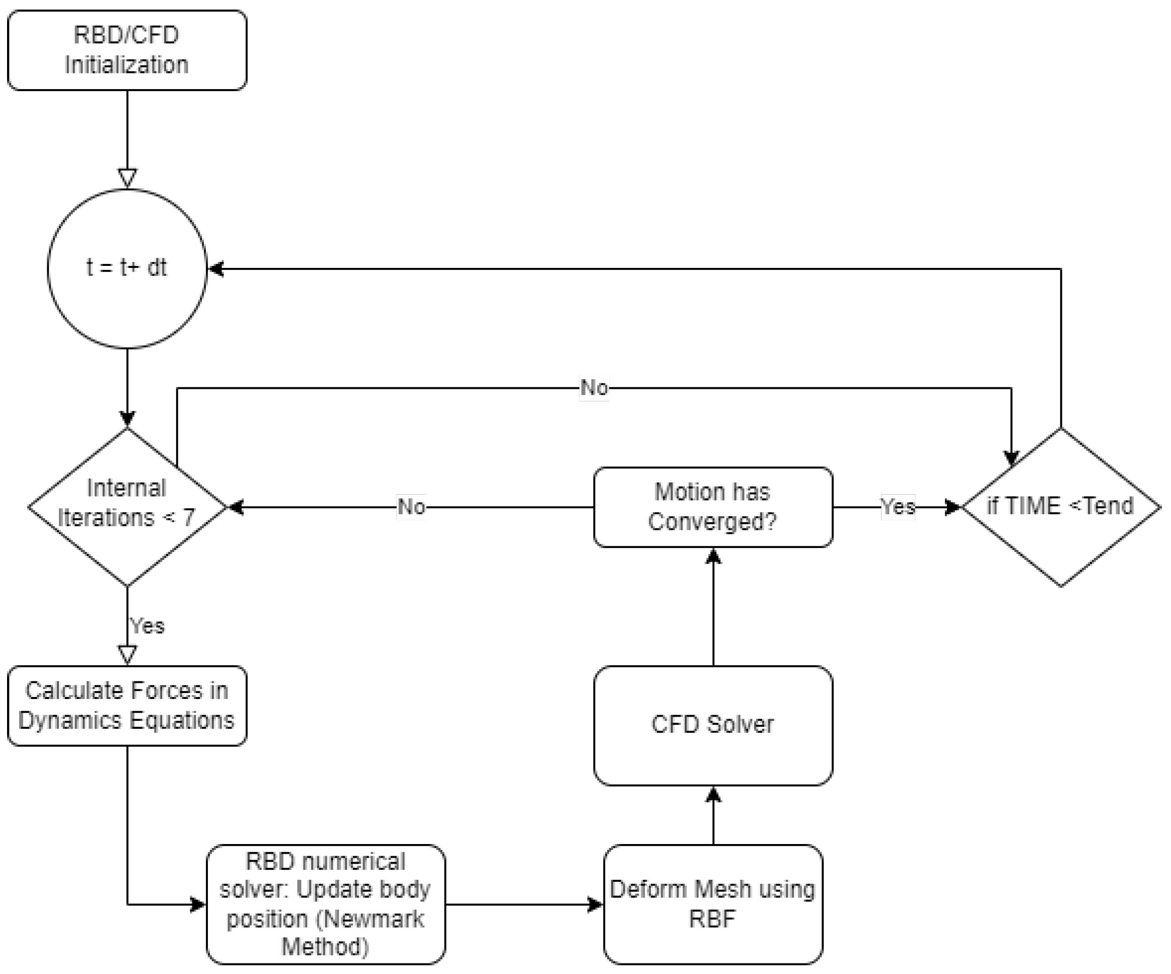
2.3. Fluid Structure Interaction

This section briefly describes the fluid-structure interaction (FSI) methodology. The energy harvesting foil is fully passive and thus it’s motion is driven by the forces exerted on it by the surrounding fluid. The study focuses on 2D approach with heave and pitch degrees of freedom. The dynamics system is modelled using Equation (20).

$$M\ddot{\overrightarrow{x}}\left(t\right)+C\dot{\overrightarrow{x}}\left(t\right)+K\overrightarrow{x}\left(t\right)={\overrightarrow{F}}_{tot}\left(t\right)$$

(20)

where $\overrightarrow{x}$ is the 1D vector of displacements for the heaving and pitching DOFs, M the mass matrix, C the damping matrix and K the stiffness matrix. The vector ${\overrightarrow{F}}_{tot}=(F_2,M_3)$ includes the total excitation forces and moments of the system.

The excitation forces and moments of the system are the integrated pressure and viscous forces over the wall boundary, given in (20), where $\overrightarrow{r}$ is the respective lever arm from the device’s center of gravity.

$$\begin{array}{c}{F}_2={\oint }_{\partial B}p{n}_y+\left(\overline{\tau }·\overrightarrow{n}\right)n_y\mathrm{dS}\\ M_3={\oint }_{\partial B}\left(p\overrightarrow{n}+\overline{\tau }·\overrightarrow{n}\right)\times \overrightarrow{r}\mathrm{dS}\end{array}$$

(21)

where p and $\tau$ are the pressure and shear stress acting on the body, $\overrightarrow{n}$ and ${\overrightarrow{n}}_y$ tangential and vertical unit vectors and $\overrightarrow{r}$ the moment lever. In FSI problems, the non-linear Equation (20) needs to be linearized to be solved iteratively. This linearization is performed during the pseudo-timesteps, and it allows the system to be solved more efficiently. In this work after each pseudo-timestep, the flow solver provides the forces and moments to the rigid dynamics solver (RBD), which then numerically integrates (using the the Newmark-$\beta$ method) the equation of motion to compute the new position of the body. This iterative procedure results in a strong coupling between the fluid solver and the rigid body dynamics solver. A schematic representation of the algorithm used in FSI simulations is shown in Figure 1.

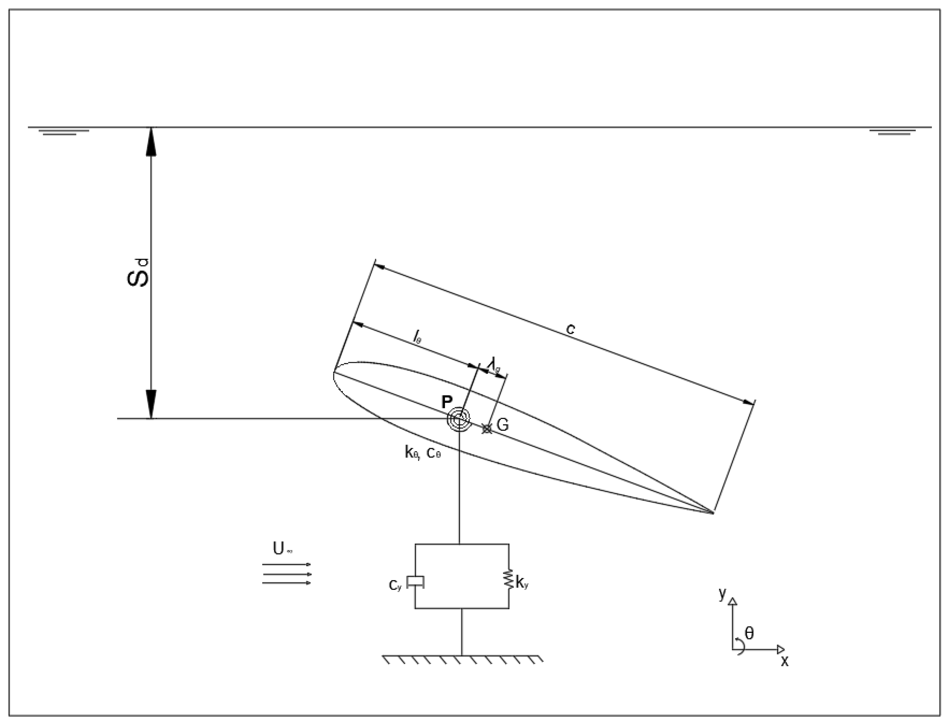
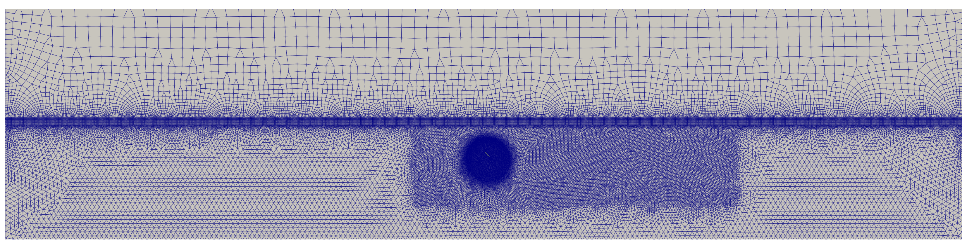
3. Basic Numerical Setup

The schematic of the fully passive flapping foil device is given in Figure 2. In this work we examine the flapping foil in two dimensions and consequently the foil has three degrees of freedom (DOFs), namely surge, heave and pitch. The device is comprised of a foil with chord length c. Fluid flow is horizontal and uniform, with a magnitude of $U_{\infty }$, rightwards, as shown in the figure, while gravity acts vertically, downwards. The foil is attached to linear springs and dampers in the heaving and pitching degrees of freedom, and its movement along the surge DOF is neglected. The corresponding stiffness for each spring is $k_y$ and $k_{\theta }$ and the damping coefficients are $c_y$ and $c_{\theta }$ for the heaving and pitching DOFs, respectively. The pitching axis is located at the point P which lies on the chord line of the foil, located at a distance $l_{\theta }$ from the leading edge. We also denote the distance ${\lambda }_G$ from the point P to the center of gravity G (CoG) of the device’s moving parts. A positive value of ${\lambda }_G$ means that the center of gravity is located downstream of the pitching axis. The pitching axis generally differs from the CoG, which gives rise to the so called static imbalance defined in (22). This static imbalance couples the two DOFs and allows energy transfer between them. The parameter of submergence depth ($S_d$) is also defined in Figure 2 as the distance from the foil’s pitching axis to the free surface, when the springs are not deformed.

$$\begin{array}{c}\hfill \Lambda ={\lambda }_g{m}_{\theta }\end{array}$$

(22)

Hydrodynamic and linkage loads (springs and dampers), along with inertial forces act on the foil. Applying Newton’s second law, two nonlinear coupled differential equations arise, for the heaving and pitching DOFs, given in (23) and (24) [44].

$$\begin{array}{cc}\hfill & m_y\ddot{y}+c_y\dot{y}+k_{y}y+\Lambda ({\dot{\theta }}^{2}sin\theta -\ddot{\theta }cos\theta )=F_y\hfill \end{array}$$

(23)

$$\begin{array}{cc}\hfill & I_{\theta }\ddot{\theta }+c_{\theta }\dot{\theta }+k_{\theta }\theta -\Lambda \left(\ddot{y}cos\theta \right)=M_{\theta }\hfill \end{array}$$

(24)

where $m_y$ is the heaving mass, $m_{\theta }$ is the pitching mass and $I_{\theta }$ the moment of inertia of the foil with respect to the pitching axis, which is located at P and is perpendicular to the x-y plane. $m_y$ and $m_{\theta }$ might differ, since some mechanical components may participate only in one of the two motions. In the right side of the equations, $F_y$ is the hydrodynamic force acting on the heave direction and $M_{\theta }$ is the hydrodynamic moment with respect to the pitching axis. The non-dimensional form of the structural parameters used is given in

Table 1. Definition of non-dimensional parameters used in the present study.

Parameter	Definition	Parameter	Definition
$Re$	$\frac{U_{\infty }c}{\nu }$	$m_{\theta }^{\ast }$	$\frac{m_{\theta }}{\rho b{c}^2}$
$m_y^{\ast }$	$\frac{m_y}{\rho b{c}^2}$	${\Lambda }^{\ast }$	${\lambda }_g$$m_{\theta }$
$k_{\theta }^{\ast }$	$\frac{k_{\theta }}{\rho U_{\infty }^{2}b{c}^2}$	$c_{\theta }^{\ast }$	$\frac{c_{\theta }}{\rho U_{\infty }b{c}^3}$
$k_y^{\ast }$	$\frac{k_y}{\rho U_{\infty }^{2}b}$	$c_y^{\ast }$	$\frac{c_y}{\rho U_{\infty }bc}$
$I_{\theta }^{\ast }$	$\frac{I_{\theta }}{\rho b{c}^4}$	$l_{\theta }^{\ast }$	$\frac{l_{\theta }}{c}$

.

The dampers effectively replicate the load on the foil from an electric generator, and since the power extracted can be calculated through $c_{\theta }$ and $c_y$ we proceed to define an efficiency coefficient to assess the foil performance. The hydraulic efficiency ($\eta$) is therefore defined as the integral of the ratio of power harvested divided by the hydraulic power available in the flow area S.

$$\begin{array}{c}\hfill \eta =\frac{1}{\Delta t}{\int }_{t_0}^{t_0+\Delta t}\frac{c_y{\dot{y}}^2+c_{\theta }{\dot{\theta }}^2}{\frac{1}{2}\rho U_{\infty }^{3}S}dt\end{array}$$

(25)

where S is the maximum cross-sectional area swept by the foil, defined by the product of the foil’s span, b, and the total vertical flow distance scanned by the foil.

Another useful metric can be defined normalizing the hydraulic power in terms of the projected surface of the foil ($b\times c$). Consequently, the average power coefficient (${\overline{C}}_p$) is defined as:

$$\begin{array}{c}\hfill {\overline{C}}_p=\frac{1}{\Delta t}{\int }_{t_0}^{t_0+\Delta t}\frac{c_y{\dot{y}}^2+c_{\theta }{\dot{\theta }}^2}{\frac{1}{2}\rho U_{\infty }^{3}bc}dt\end{array}$$

(26)

Finally, the main parameters chosen for the fully passive flapping foil device, are given in their non-dimensional form in

Table 2. Parameters used in the present study.

Parameter	Value	Parameter	Value
$Re$	$6\times {10}^4$
$m\ast$	0.92	${\Lambda }^{\ast }$	0.0065
$k_{\theta }^{\ast }$	0.071	$c_{\theta }^{\ast }$	0.052
$k_y^{\ast }$	0.72	$c_y^{\ast }$	0.93
$I_{\theta }^{\ast }$	0.0563	$l_{\theta }^{\ast }$	0.33

(taken from [45]). In the case studied in this work, $m_y^{\ast }$ and $m_{\theta }^{\ast }$ are both equal to $m^{\ast }$.

Dimensionless force and power coefficients for each DOF are also defined in (27) in order to aid in the analysis of the results. $P_{F_y}$ is the power extracted from the heaving motion and $P_{M_{\theta }}$ from the pitching motion.

$$\begin{array}{c}\hfill C_L=\frac{F_y}{\frac{1}{2}\rho U_{\infty }^{2}bc}{C}_M=\frac{M_{\theta }}{\frac{1}{2}\rho U_{\infty }^{2}b{c}^2}\\ \hfill C_{P_y}=\frac{P_{F_y}}{\frac{1}{2}\rho U_{\infty }^{3}bc}{C}_{P_{\theta }}=\frac{P_{M_{\theta }}}{\frac{1}{2}\rho U_{\infty }^{3}b{c}^2}\end{array}$$

(27)

In [23], the grid and time step requirements are investigated based on the comparison with measurements. Since in this work the foil operates beneath the free surface, a new grid independence study is carried out. The grid in the near airfoil region and the wake refinement zones remain approximately the same as the ones presented in the [23]. Consequently, the focus of this study concerns the mesh resolution near the free-surface region.

For the grid independence study, we consider the case of $S_d$ = 4c and Fr = 1. Three successively refined grids in the vicinity of the free surface are generated and results are compared in terms of the passive motion characteristics. The coarse grid has a horizontal spacing $\Delta$x = 0.24c and vertical spacing of $\Delta$y = 0.04c. The medium fidelity grid has a spacing $\Delta$x = 0.12c, $\Delta$y = 0.02c while the finest one has a $\Delta$x = 0.04c with $\Delta$y = 0.02c. It is noted here that the mesh in the free surface region is mostly structured-like.

The relative error with respect to the finest mesh of the heaving and pitching amplitudes are presented in

Table 3. Free Surface grid independence study relative errors (%) with respect to the finer grid.

Grid	${\mathit{h}}_0^{\ast }$	${\mathit{\theta }}_0^{\ast }$
Coarse	$4.34\%$	−$2.52\%$
Medium	$1.84\%$	−$1.87\%$
Fine	-	-

.

A mesh snapshot can be seen in Figure 3. At the right end of the computational domain a damping zone is employed. On the left end of the computational domain either a damping region or a wave generation zone is defined, depending on the desired simulation conditions.

Following the grid independence study, the medium fidelity mesh used for the rest of the work which consists of around $200,000$ cells with refinements in the wake region to capture the vortex shedding. In the near wall region the first cell size is selected so that $y+\le 1$ while the time step chosen is $\Delta t=0.0002 \mathrm{s}$. No initial perturbation is required to initiate the motion. Results are collected after enough periods have elapsed and the motion has sufficiently converged. The metrics used to evaluate performance are averaged across many periods, as due to the passive nature of the flapping foil, the motion and the forces that act on the foil can vary from cycle to cycle. This is especially the case when the submergence depth is small, and the free surface influences the device, as the state of the free surface differs from cycle to cycle. For each case, results from 10 cycles were averaged to obtain values for the performance metrics.

When incoming waves are considered the free surface region discretization is changed depending on the wave length and the wave heigh. More specifically, it is horizontally refined to have about 100 points per wavelength and 20 points per wave height ($H=0.2c$) (see [30]).

4. Results and Discussion

In this section the aforementioned numerical setup of the fully passive flapping foil device is used to examine the influence of the free surface when it is calm (Section 4.1) or when waves are propagating on it (Section 4.2). A parametric study is initially carried out, altering the submergence depth of the foil ($S_d$). This analysis is repeated for various Froude numbers (Fr), which is defined as:

$$\mathrm{Fr}=\frac{U_{\infty }}{\sqrt{g·c}}$$

(28)

The impact of these parameters to the performance is assessed, and their influence explained. Subsequently, the influence of monochromatic waves that propagate on the free surface is examined.

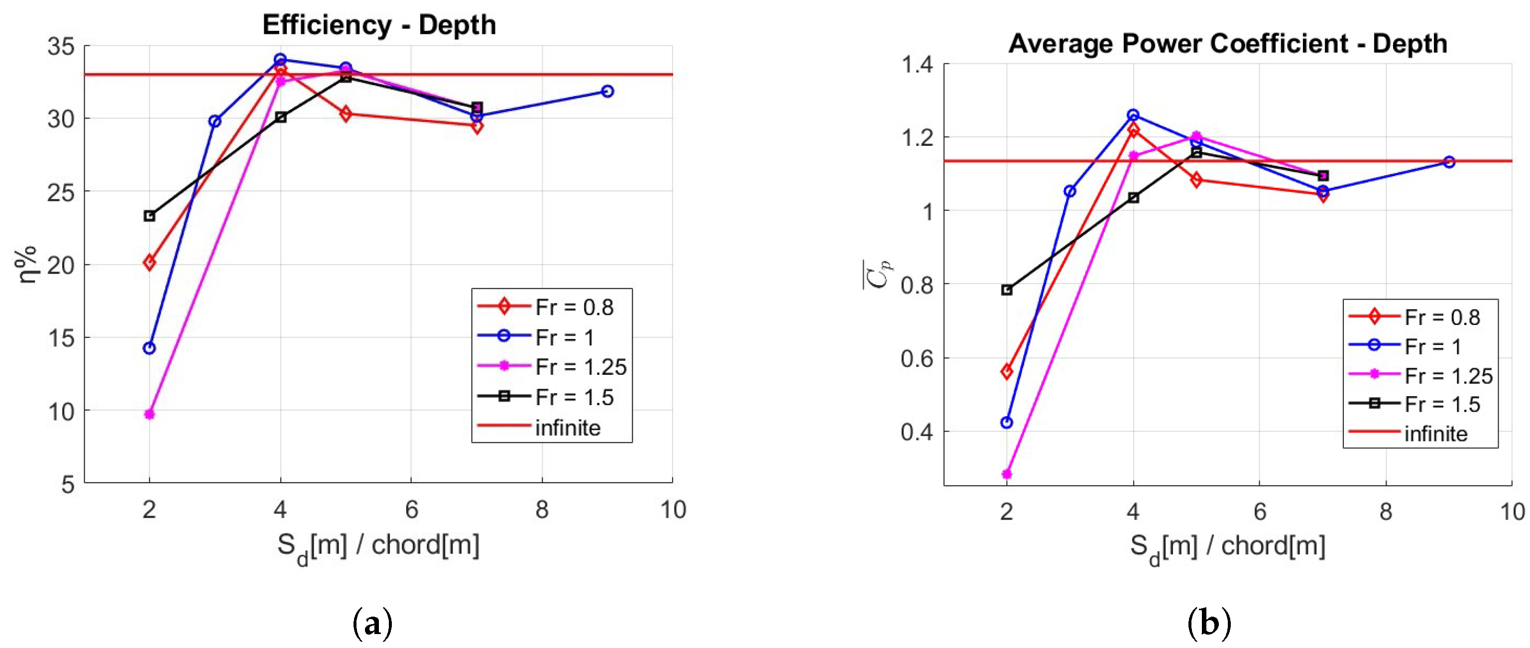
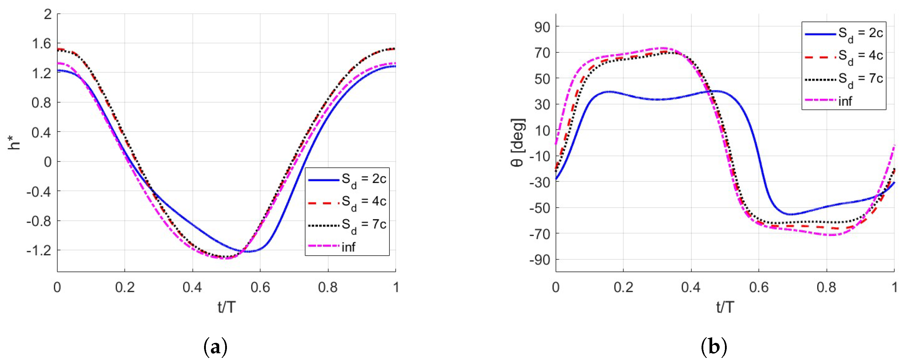
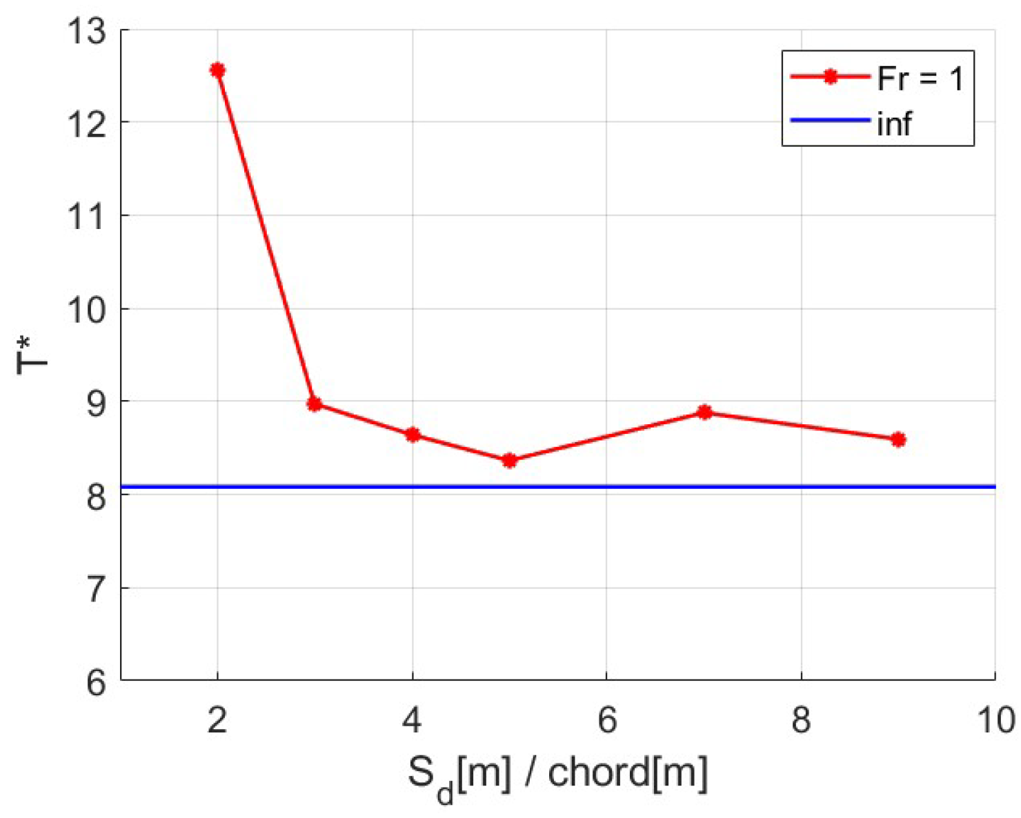
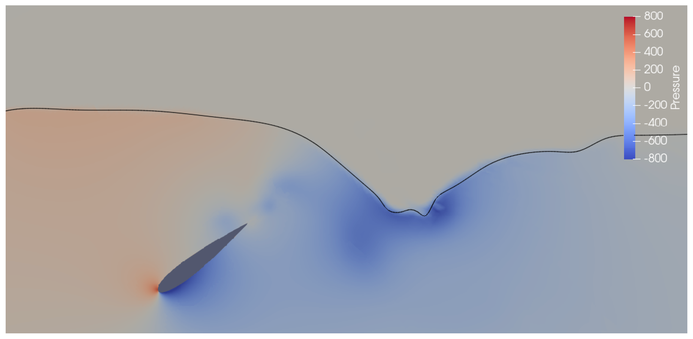
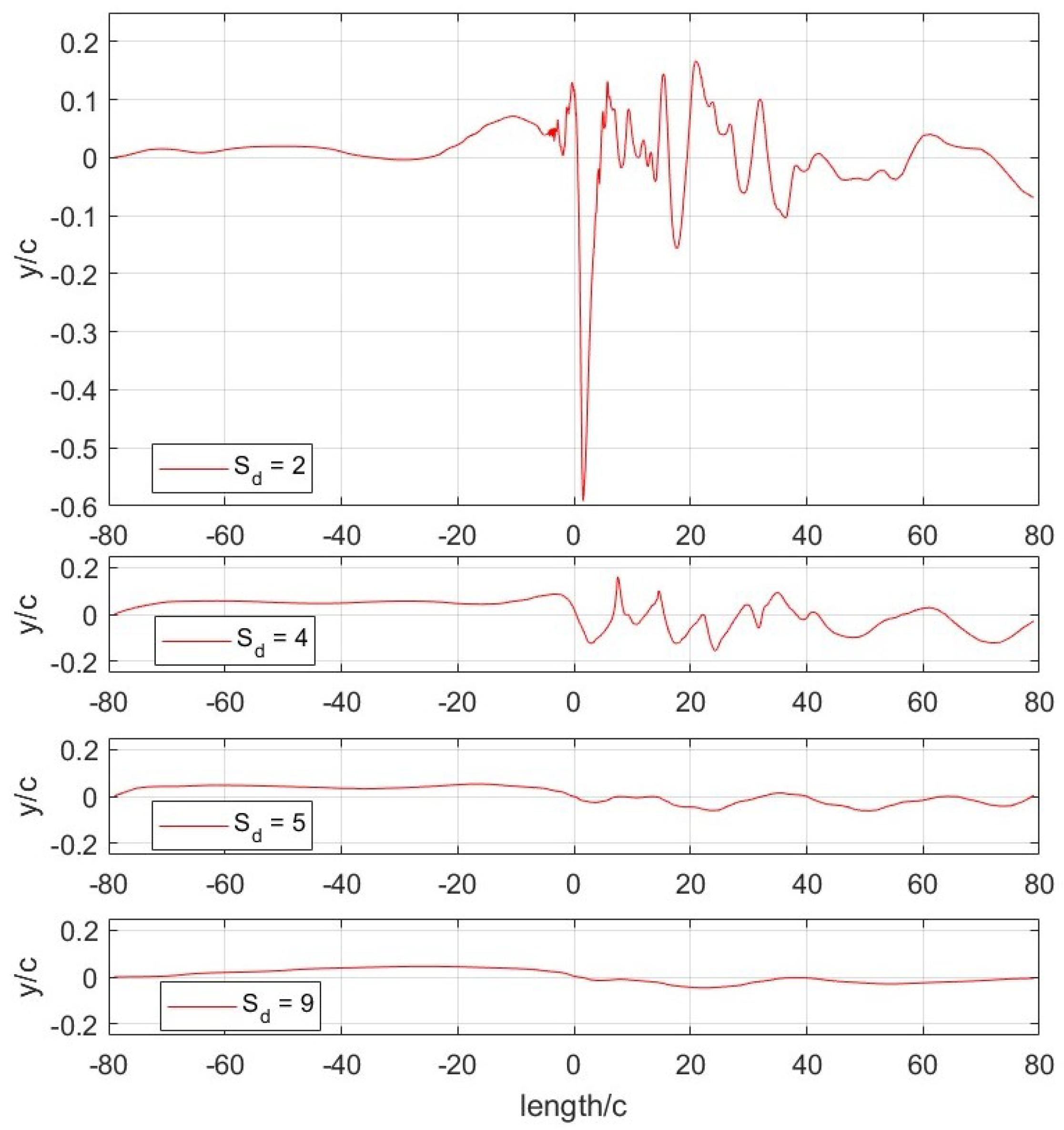
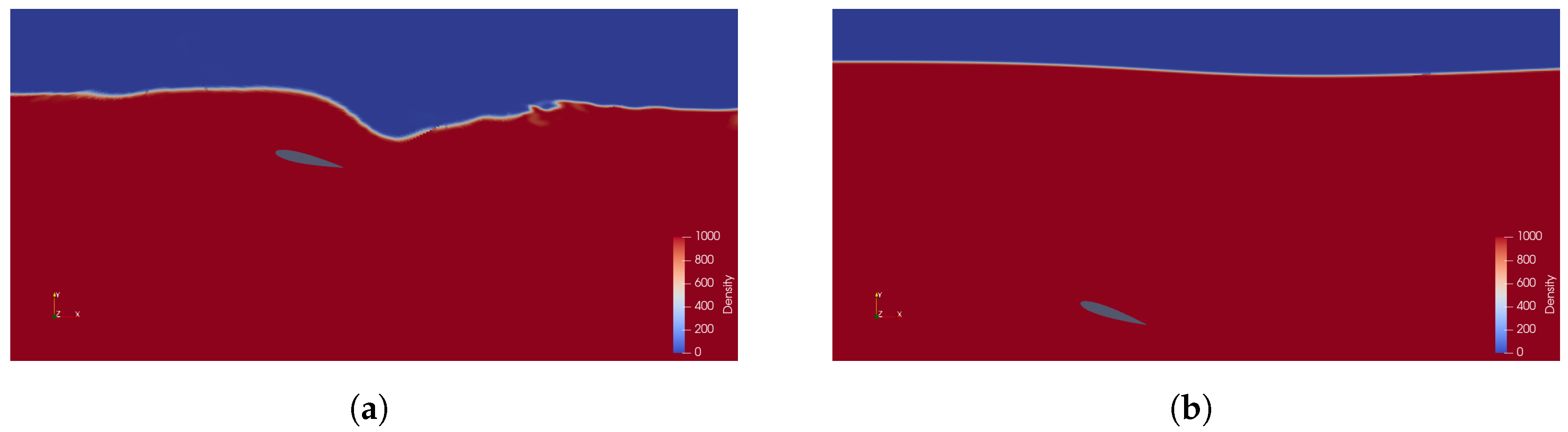
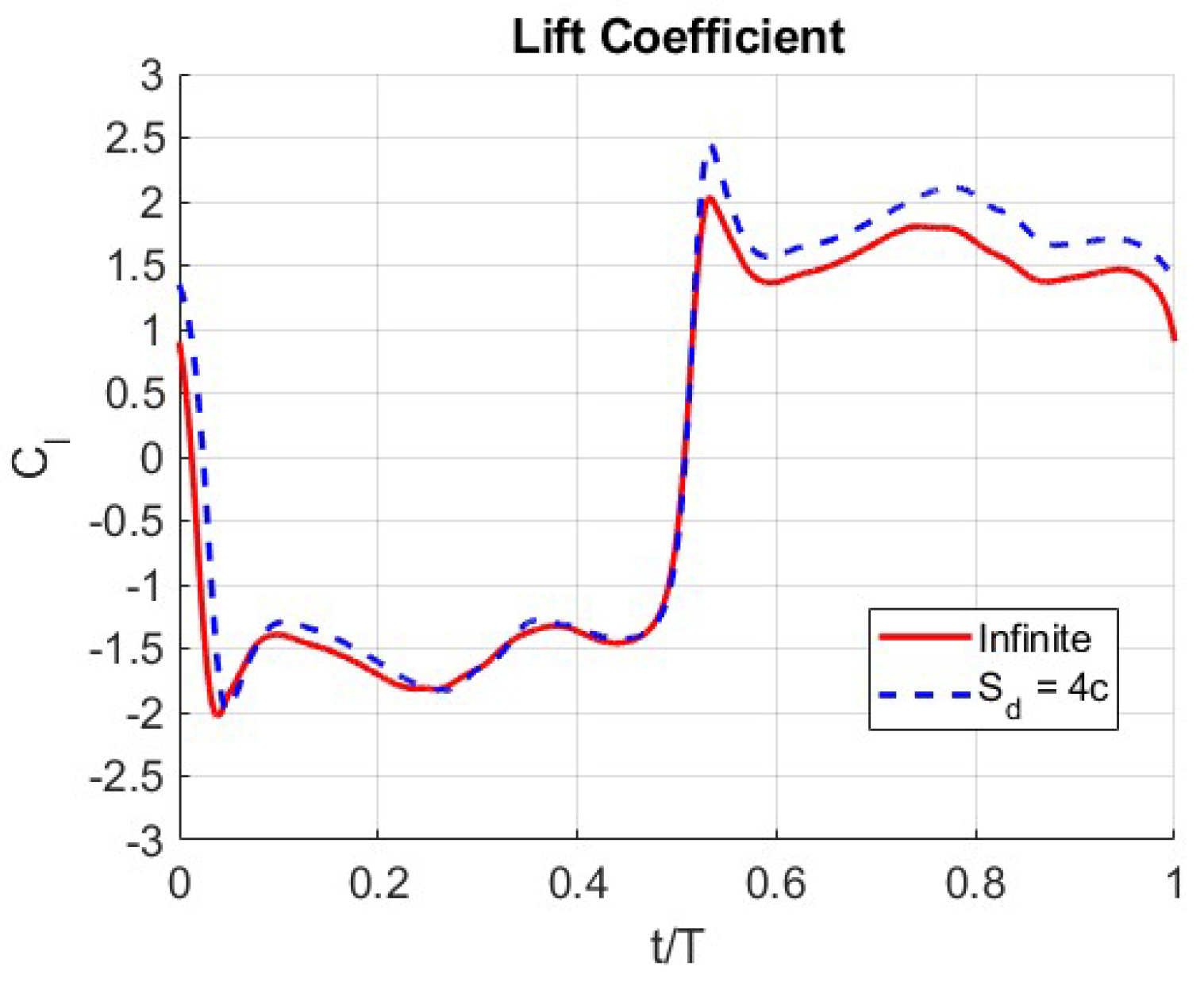
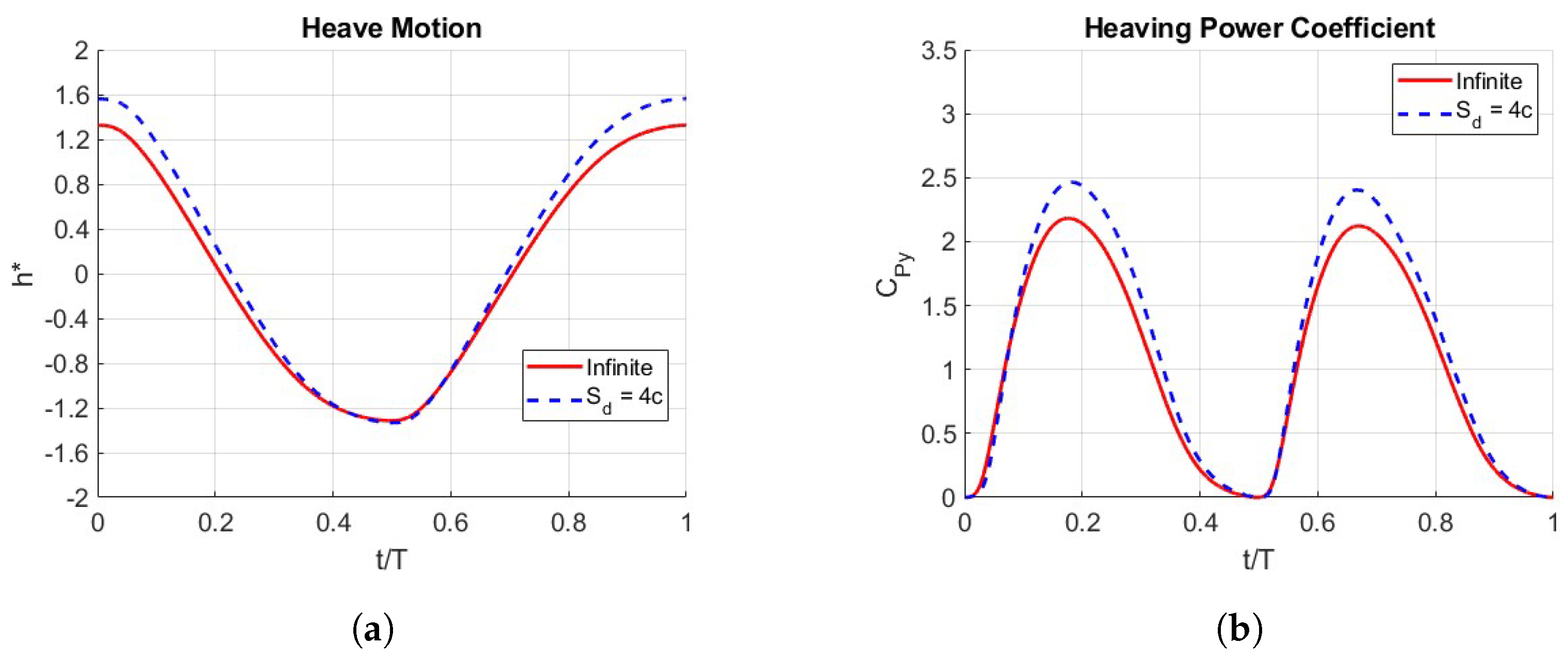
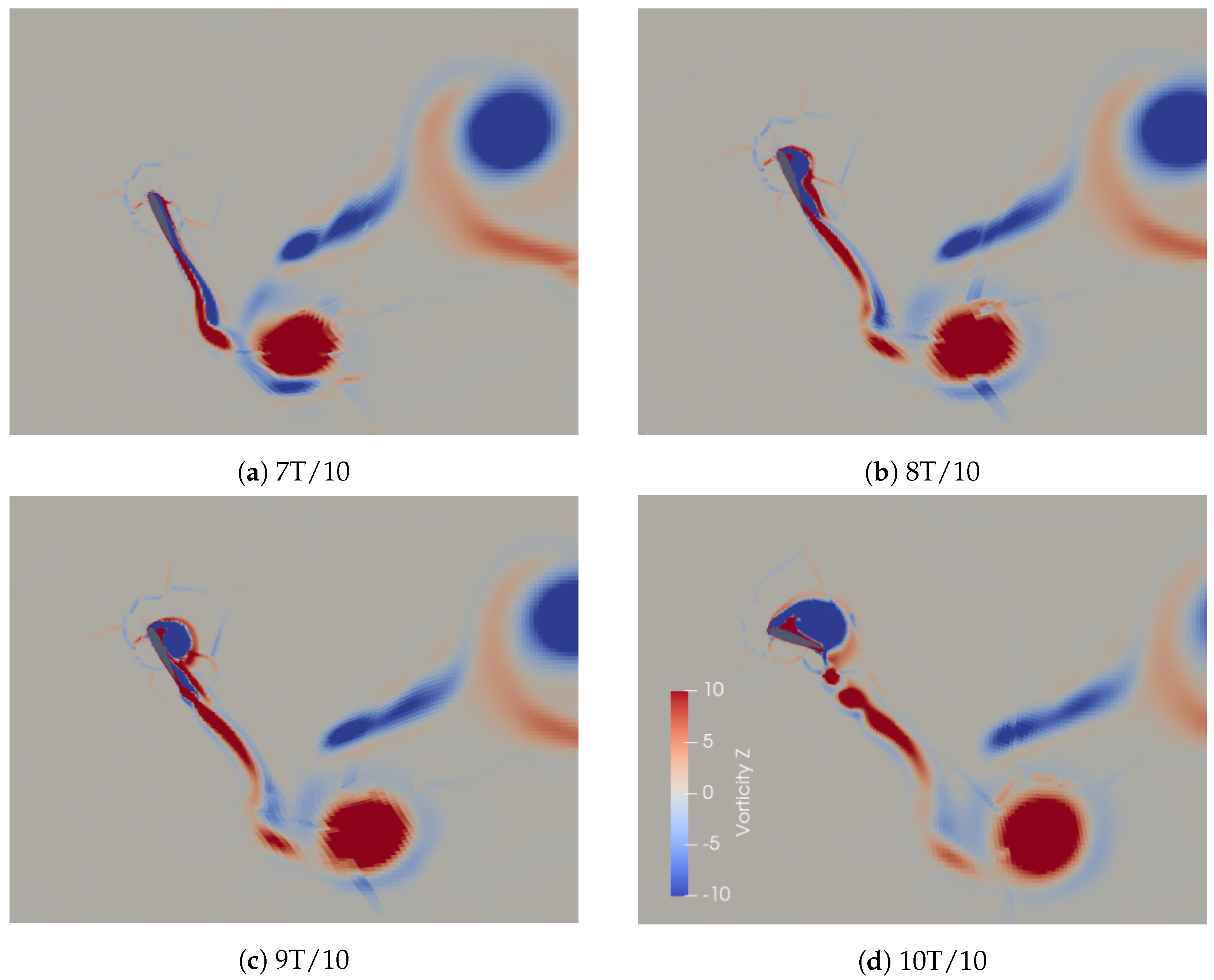
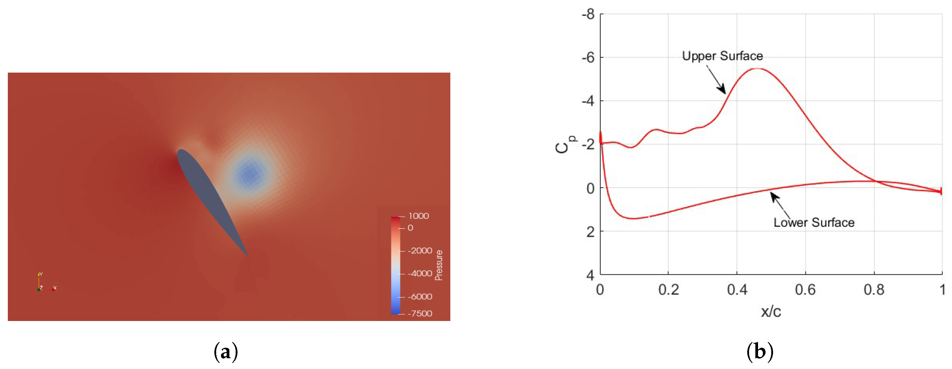
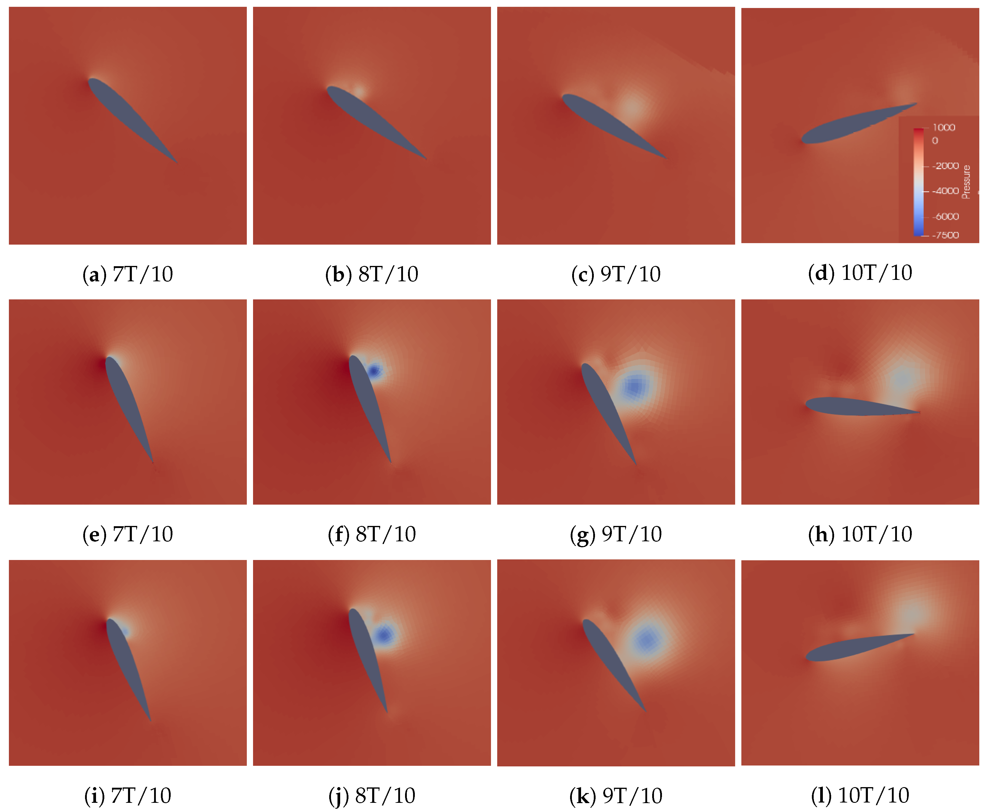
4.1. Effects of Submergence Depth for Various Froude Numbers

The effects of varying the submergence depth ($S_d$) are examined in this section. Apart from the submergence depth, the Froude number also affects the performance of this device when considering the influence of the free surface, as both the dynamics of the flow around the foil and the disturbance of the free surface are affected. For this reason, this same analysis is carried out for multiple Fr numbers, Fr = 0.8, 1, 1.25, 1.5. The performance of the device is assessed using two metrics, efficiency $\eta$ and average power coefficient $\overline{C_p}$, described in Section 2. In Figure 4a,b, the results for all the cases examined are presented. Each curve in the $\eta -S_d$ and $\overline{C_p}-S_d$ diagrams corresponds to a different Fr number. The horizontal red line represents the infinite depth case (no free surface influence) as a comparison to the other cases. As a general trend, we notice that for low submergence depths, below three chord lengths (c), performance drops rapidly as the foil is very close to the free surface. For intermediate $S_d$, a maximum appears for all the Fr numbers, where $\eta$ and $\overline{C_p}$ are as high or even higher than the infinite depth case. Increasing $S_d$ further, performance drops again until it approaches asymptotically the infinite depth case.

Results indicate that there exists an optimal $S_d$ where the calm free surface not only does not decrease performance relative to the infinite case, but also a slight increase is evident. The exact depth $S_d$ that the maximum occurs depends on the Fr number. As Figure 4 indicates even though the Fr number can affect performance the efficiency maximum can be found at intermediate $S_{d}s$ (between 4c–5c). This happens because of a beneficial mechanism, described in the “Free Surface Flow Constriction” section, that outweighs the negative effects of the other mechanisms described later in this work.

Effects of Submergence Depth for Fr = 1

To better understand the effect of submergence depth and the underlying fluid mechanics phenomena, we focus our study to Fr = 1. The submergence depths examined for the specific Fr number are $S_d=2,3,4,5,7$ and 9 chord lengths.

The main metrics for each submergence depth, for Fr = 1 are presented in

Table 4. Fr = 1: Main Metrics for various Submergence Depths.

Metrics/${\mathit{S}}_{\mathit{d}}$	$2\mathit{c}$	$3\mathit{c}$	$4\mathit{c}$	$5\mathit{c}$	$7\mathit{c}$	$9\mathit{c}$	Infinite
$h_0^{\ast }$	1.26	1.45	1.44	1.40	1.40	1.41	1.32
${\theta }_0^{\ast }$ (deg)	47.7	66.3	71.8	70.7	65.7	67.9	72.2
$\eta \%$	14.25	29.67	34.10	33.42	30.13	31.83	32.98
$T^{\ast }$	12.6	9.0	8.3	8.4	8.9	8.6	8.1
$\overline{C_p}$	0.42	1.06	1.26	1.19	1.05	1.13	1.13

, where $h_0^{\ast }$ and ${\theta }_0^{\ast }$ are heaving and pitching amplitudes (heave is non-dimensional by chord length c and $\theta$* is in degrees) and T* is non-dimensional period ($T^{\ast }=T·U_{\infty }/c$).

As Table 4 suggests, the influence of the free surface is not straightforward. Efficiency and Power Coefficient seem to have a similar behaviour. For high $S_d$, such as $S_d=7c$ and $9c$ the presence of the free surface slightly reduces the performance of the device. The influence is small as the infinite case is approached for high $S_d$. For very low $S_{d}s$ close to $2c$ performance is largely reduced. The hydrofoil is very close to the free surface and large amounts of energy are expended to the formation of waves. Other reasons, relating to the behaviour of the vortices around the foil affect its performance, and are discussed later in this section.

In Figure 5a,b, the heaving and pitching motions can be found, for $S_d=2c,4c,7c$. It is evident that the heaving amplitude ($h_0^{\ast }$) is not significantly affected when the foil is at low $S_{d}s$. The pitching amplitude, in contrast, is significantly decreased. Figure 5 can reveal a lot about the hydrofoil’s performance. It shows how the heaving and pitching motion timeseries of the fully passive flapping foil device stray away from a pure sinusoidal motion. The influence of submergence depth on it is compared for different cases, where we see that for intermediate submergence depths the motion is not significantly altered. Interestingly, compared to the infinite fluid case, the heaving amplitude is increased during the upstroke but is the same during the downstroke. Additionally, it shows that for the $S_d$ = 2c case, pitching is greatly reduced throughout the cycle, indicating that the lifting force acting on the foil is reduced and in consequence performance is decreased. In addition, in this figure an indication of the increase in phase difference between the heaving and pitching motion is also visible at t/T = 0, when the free surface is present and especially for the $S_d$ = 2c case. At this time instant, when the hydrofoil is at the uppermost position, the pitch angle is not 0° but it lags behind. Finally, comparing the $S_d$ = $4c$ and $7c$ cases, the heaving motion is almost identical, but the pitching angle is slightly reduced for the $7c$ case, which degrades performance.

Additionally, in Figure 6 the non-dimensional period $T^{\ast }$ is presented as a function of $S_d$ and compared to the infinite case (horizontal blue line). It is clear, that the period ($T^{\ast }$) is greatly increased when the foil operates near the free surface ($S_d=2c,3c$). This increased period, means that foil’s velocity is reduced and thus less energy is harvested from the foil. For intermediate $S_{d}s$, such as $4c$ and $5c$, a peak forms, and $T^{\ast }$ is very close to the reference infinite case.

Depletion of energy in waves.

The free surface directly affects the performance of the flapping foil as energy is transferred from the foil to the creation of gravity waves. As the foil approaches the surface, larger waves are formed, which means that more energy is lost in wave making. In essence, the pressure differences that the foil creates lend part of their energy to the creation of waves leading to the reduction of lift. Additionally, the formed wave system can affect the pressure distribution on the foil and thus the resulting pitching motion. This can be seen in Figure 7, which shows the hydrofoil at the $S_d$ = 2c case where the disturbance is very pronounced, close to the uppermost position. This figure shows that the formed wave system changes the pressure distribution in the region and influence the loads on the hydrofoil.

The free surface disturbance for the various $S_{d}s$ can be seen in Figure 8. We chose to present the free surface when the foil is at its uppermost position. As expected, the disturbances are larger for low submergence depths, reaching wave amplitudes up to $0.6c$. The free surface is also visualized by the density plot in Figure 9, comparing $S_d=2c$ with $S_d=4c$ when the foil is at its uppermost position, where the disturbance in the low $S_d$ case is particularly high.

It is notable, however, that even though at $S_d=4c$ significant waves are formed in the free surface, the performance of the foil is slightly increased. This signifies that free surface wave making is not the only factor affecting performance.

Free Surface Flow Construction

The second significant effect that affects performance when the foil operates near the free surface is caused due to the constriction of the flow above the foil. The pressure drop due to the constriction results in increased velocities in the region. These increased velocities along with the influence of the disturbance of the free surface, affect the pressure on the upper side of the foil.

Constriction of the flow can be beneficial for energy extraction. As the foil heaves upwards, pressure is decreased further on its upper side compared to the infinite case, causing the Lift force to increase. This means that more energy is harvested from the device. As the foil moves downwards, this effect is reversed, which means that lift is decreased compared to the infinite depth case. This is illustrated in Figure 10 for a single period, where the infinite depth case Lift Coefficient ($C_l$) is contrasted to that of the $S_d=4c$ case. In the first half-period, the magnitude of lift is slightly less but in the second half it is significantly greater. It can be seen that the increase in the absolute value of the $C_l$ on the second half of the period (upstroke) is greater than the decrease on the first half (downstroke). This explains why there is a net positive effect on the foil’s performance, at the particular $S_{d}s$.

The increased $C_l$ during the upstroke, increases the amplitude of the heaving motion, as depicted in Figure 11a (while it is the same at the downstroke). Figure 11b depicts the heaving power coefficient, where it is evident that power extraction is increased for $S_d=4c$, throughout the period. Energy extraction from the pitching motion is much less than that of the heaving motion, and it does not differ significantly between these cases.

Motion Synchronisation

Synchronisation of the heaving and pitching motion is very important in the search for structural parameters in order to achieve good performance. This device is not active, meaning that the motion is not prescribed, so the motion cannot be explicitly set. In essence, the pitching motion is responsible for the suitable positioning of the foil, so that the maximum amount of power can be harvested by the heaving motion. Consequently, when the motions in the two DOFs are not well synchronised, harvested energy decreases.

As described in [46], a large Leading Edge Vortex (LEV) is formed close to the leading edge of the foil, as the foil goes through dynamic stall, which is detached when certain conditions are met. The vorticity of the flow during an upstroke for the $S_d=4c$ case is shown in Figure 12. It can be seen, that the LEV forms, detaches, and afterwards is convected downstream along the upper surface of the body. Apart from the structural parameters, the kinematics of the LEV is a significant factor that drives the passive foil motion.

Figure 13a shows the pressure contour at 9T/10 of the motion cycle. The LEV can be identified as the low pressure area. Its effect on the foil loading can be seen in Figure 13b that shows the corresponding pressure coefficient (Cp) plot at the same time instant. It is clear that the location of the LEV results in a lower pressure region acting on the foil.

At this time instant, the LEV induced pressure drop results in a large counter-clockwise moment that acts on the hydrofoil. Consequently, the hydrofoil changes orientation so that the downstroke will begin. This mechanism determines the pitching motion and affects synchronisation.

The presence of the free surface can have favourable characteristics as well as negative ones. In the former case, the free surface acts like a solid boundary where the well-known “wing-in-ground” effect can enhance the foil performance [47]. However, free surface deforms and waves are generated so a part of the available energy is depleted. The basic parameter that affects whether the presence of free surface will enhance or degrade performance is the depth-to-chord ratio ($S_d$). Depending on $S_d$ and the interaction of the foil with the free surface the motion of the passive foil can change. A closer look at the motion dynamics reveals that the LEV has a critical role in the foil’s motion [23].

Understanding the influence of this LEV is important, because, when the hydrofoil is located close to the free surface, a delay in the pitching motion is noticed which is caused by a delay of the shedding of the LEV. This is illustrated in Figure 14 where the $S_d$ = 2 and $4c$ case is compared with the infinite case (no free surface). It is evident that as $S_d$ ratio becomes smaller a delay in the detachment of the LEV is noticed.Apart from that, it is clear that the strength of the LEV (evident as pressure drop in the plot) is greatly reduced when the foil operates very close to the free surface ($S_d$ = 2c). In addition, it is clear that in the later the maximum angle of attack is reduced due to the energy lost in wave-making leading to a weaker LEV which in turn changes the foil dynamics and a degrade in performance is evident.

Following the previous discussion, when the foil operates under the free surface we have two mechanisms opposing one another. On one hand the enhancement due to the “wing-in-ground” effect and on the other hand the wave-making losses. Thus, its expected that an optimum $S_d$ exists in which the performance gain due to “wing-in-ground” effect surpass the depleted energy. Indeed, at $S_d$ = 4c a peak in the efficiency is noted. A closer look at Figure 14, reveals that the LEV evolution is closer to the infinite flow case. The LEV is only slightly delayed while the magnitude of the vortex is slightly stronger. In other words, the heaving motion due to the “in-ground” effect is enhanced maintaining, however, the dynamics of the LEV, that drive the foil motion.

This delayed shedding is also described by [48], where they conducted simulations of cylinders close to the free surface, that showed a clear delay in the shedding frequency, caused by the restriction of the fluid flow by the free surface, which restricts the supply of fluid in the region of the vortex.

To assess the synchronisation of the heaving and pitching motions, as $S_d$ varies, Fourier analysis was conducted to find their phase difference. These were then compared to the infinite case. The heaving and pitching motion time series were analysed and their corresponding phases were subtracted in order to find their phase difference. Results are presented in Figure 15.

These results inversely correlate with the results for the performance ($\eta$ and $\overline{C_p}$) of the foil in Figure 4a,b. For $S_{d}s$ where performance is maximised ($S_d$ = 4c, 5c), phase difference is close to the infinite case. For $S_d=7c$ phase difference is larger, and performance drops. For lower submergence depths ($S_d$ = 2c, 3c) phase difference becomes much larger as performance drops rapidly. This shows that when the foil is located very close to the free surface, the synchronisation is negatively affected, due to the delay in the shedding of the LEV. In essence, due to the bad synchronisation, the loads applied on the hydrofoil by the flow are lower, and the harvested energy decreases.

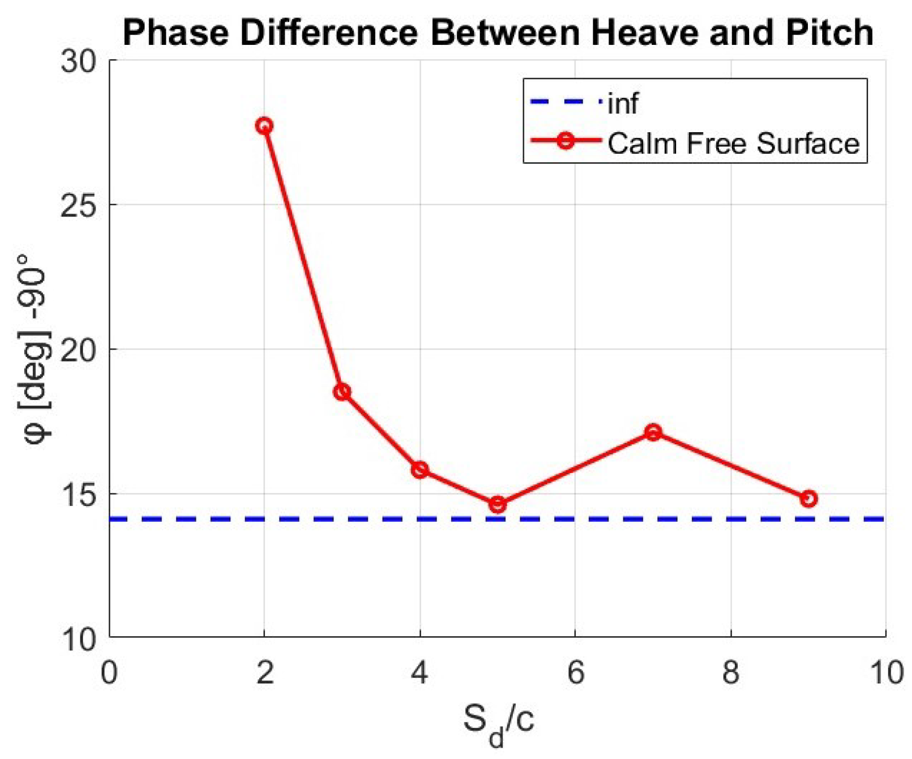
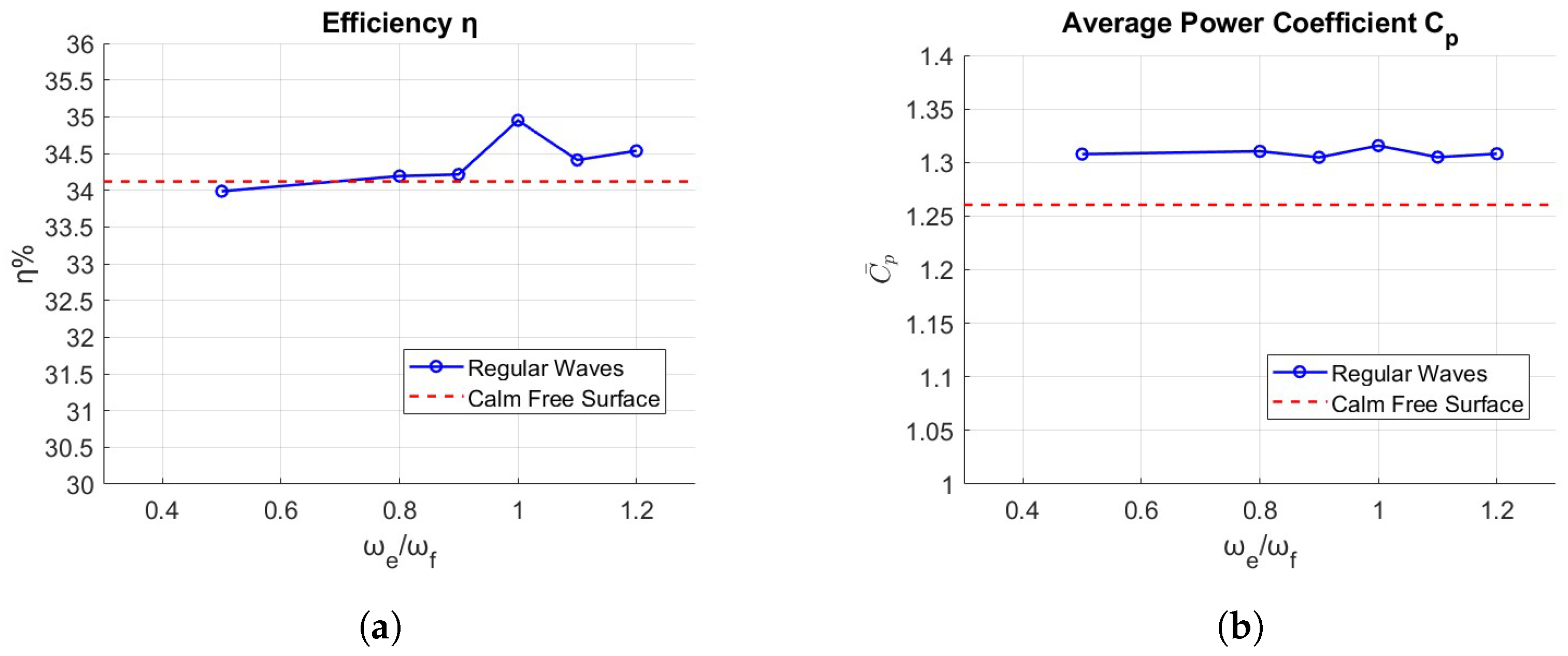
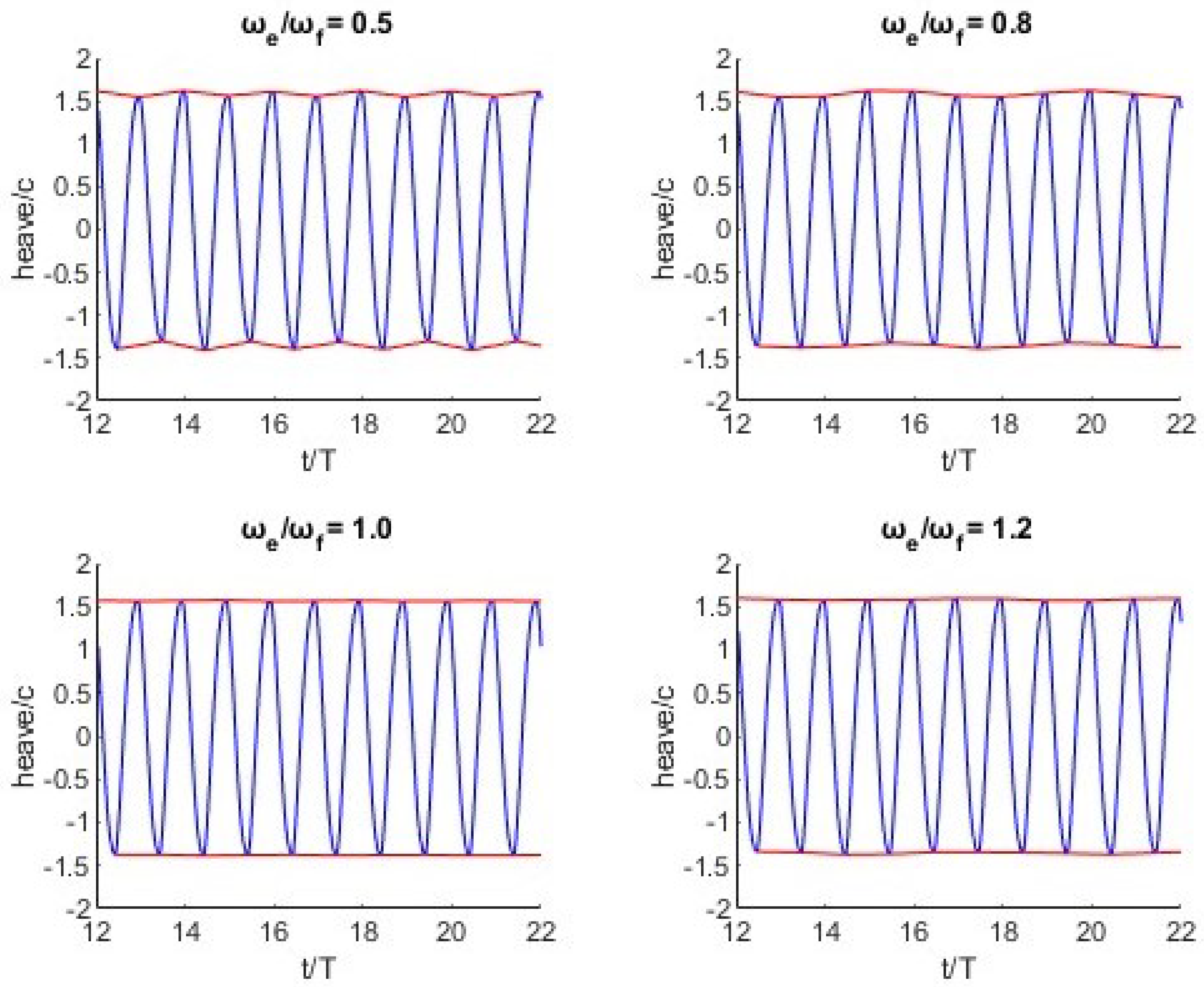
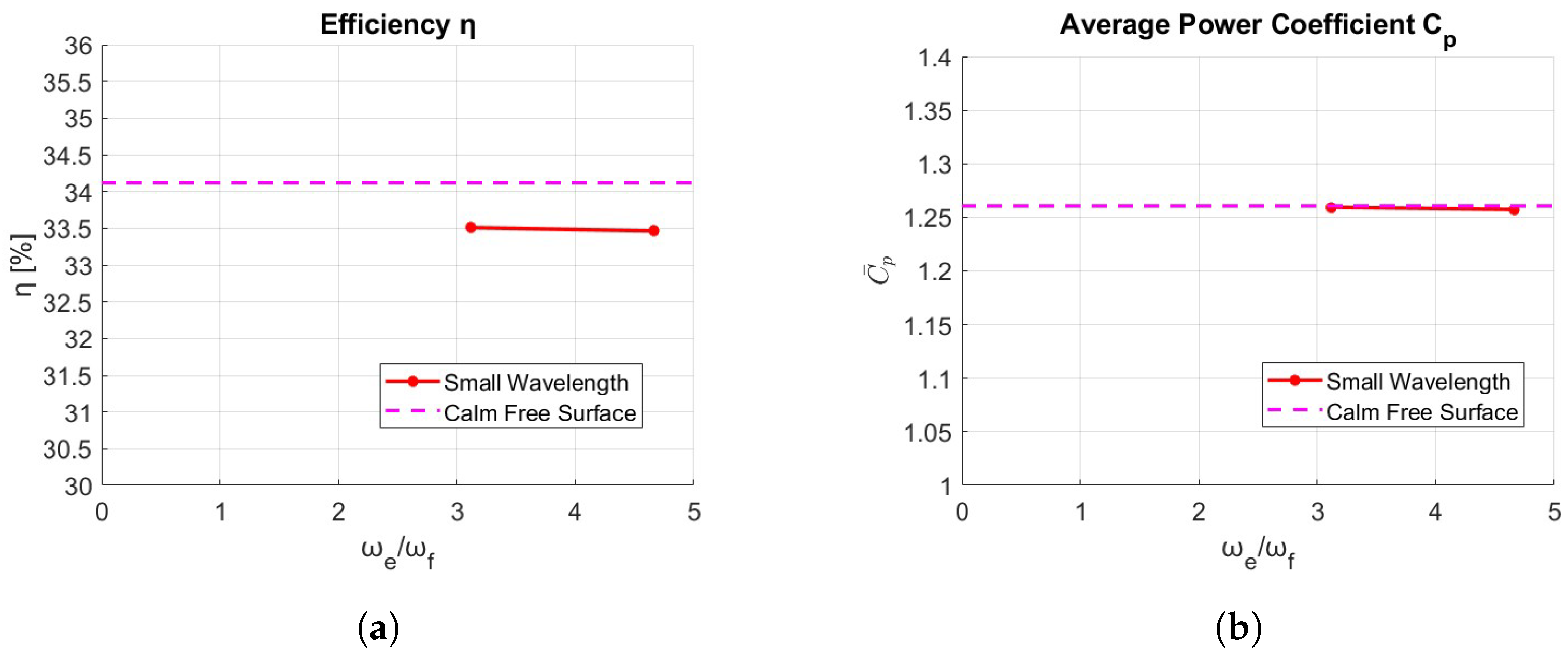
4.2. Effects of Monochromatic Waves

After examining the effects of a calm free surface on the performance of the fully passive flapping foil device, a parametric study is undertaken to examine the influence of monochromatic waves. The device is expected to operate near the free surface and consequently waves can affect its performance.

In particular, a parametric study takes place varying the frequency of these waves. The waves have frequency (${\omega }_w$), wavelength ($\lambda$) and wavenumber (k). The waves are generated using stream function theory [49]. They are generated from the left end of the computational domain using a wave-generation zone and propagate towards the passive foil. Following Section 4.1 the submergence depth $S_d=4c$ is selected, since, at this depth efficiency is maximised. Reynolds number is still $6·{10}^4$ and Fr = 1 was chosen. The device’s structural parameters and the mesh are also kept the same as in Section 4.1.

Wave frequency close to oscillation frequency

As a first step, waves that have a frequency close to the oscillation frequency of the flapping foil under a calm free surface were tested. The following ratios (

Table 5. The investigated wave frequencies and wavelengths (in airfoil chords), and the predicted non-dimensional heaving amplitudes h* = h/c.

${\mathit{\omega }}_{\mathit{w}}/{\mathit{\omega }}_{\mathit{f}}$	$\mathit{\lambda }$	Heave Amplitude ${\mathit{h}}_0^{\ast }$
calm	–	1.44
0.5	$77.3c$	1.46
0.8	$38.9c$	1.50
0.9	$32.4c$	1.44
1.0	$26.1c$	1.48
1.1	$23.9c$	1.48
1.2	$21.0c$	1.48

) of ${\omega }_w/{\omega }_f$ are investigated, where ${\omega }_f$ is the frequency of the flapping foil under a calm free surface.

The wave height $H=2A$ (A: amplitude) has to be comparable to the disturbance of the free surface caused by the foil. For this reason, it was chosen equal to $0.2c$$(A=0.1c)$ for all cases. The tank has a depth of 18c which is large relative to the wavelengths. This means that wave propagation happens in deep water conditions. The corresponding wavelengths can be seen in Table 5. Finally, it is noted that the selected wave height classifies the waves in the non-linear region.

In Figure 16, the performance of the passive foil operating in waves can be found. Figure 16a, indicates that the presence of waves does not affect efficiency significantly, except for the case of ${\omega }_w/{\omega }_f=1$, where a slight increase of about 0.8% is witnessed. This indicates that resonance of the two motions increases power extraction.

On the contrary, in Figure 16b it is seen that the average power coefficient is increased for all cases, by about the same amount, 4.5%. This suggests that the harvested power due to the presence of waves is increased. The presence of waves causes an increase in heaving amplitude as indicated in Table 5. This also explains the smaller changes in the efficiency of the device since $\eta$ is normalized by the swept area, which also increases as heaving amplitude is increased.

Figure 17 shows the heaving motion timeseries for different cases, where the peaks and crests are connected with a curve (envelope), in order to show the periodical variability of the heave amplitude, which differs for each case. This shows that the positioning of the wave relative to the foil’s motion has an effect on its motion. The variability is especially visible in the ${\omega }_w/{\omega }_f$ = 0.5, where the heaving amplitude is the same at every other cycle, as is the positioning of the wave. Figure 18 compares the heaving motion for this case to the surface elevation above it. For a particular cycle, when a wave peak is present above the foil, heaving amplitude is greater than when a crest is present. In contrast, when the frequencies of waves and flapping foil match, heaving amplitude remains stable from cycle to cycle, as in the ${\omega }_w/{\omega }_f$ = 1 case.

Wavelength close to flapping foil’s chord length.

Finally, waves with wavelength close to the foil chord are examined. Two cases of waves with wavelength comparable to the chord length of the foil are investigated, namely $\lambda =3c$ and $5c$. The pressure field caused by these waves varies along the chord length of the foil, in contrast to the previous investigations, where at a time instant, the pressure field of the wave is uniform along the foil. Their frequency is also much larger than previously.

Results are presented in Figure 19a,b with red markings relative to the calm free surface case. First a very slight decrease in efficiency of about 0.6% is evident for small wavelengths, while the gain in Power Coefficient ($\overline{C_p}$) from the previous cases with waves is lost, as power extraction is the same as in the calm free surface case. This shows that waves with wavelength close to the hydrofoil’s chord length do not aid energy harvesting, as do waves with frequency close to its frequency. Thus, compared to waves with frequency close to the flapping foil’s frequency that were examined previously, these small wavelength and high frequency waves do not aid energy harvesting, but they also do not hinder it, as the drop in performance is insignificant.

5. Conclusions

In conclusion, the performance of a fully passive flapping foil device for energy harvesting was investigated in a free surface flow through a series of numerical simulations. We used a strongly coupled FSI algorithm to examine the effects of varying submergence depths and the impact of monochromatic waves on the foil’s performance.

The results showed that the fully passive flapping foil device can achieve high efficiency for submergence depths between $4c$ and $9c$. It is notable that there is an “optimum” submergence depth where the flapping foil performance is maximised. The device had its maximum performance at a submergence depth of $4c$ with efficiency equal to 34.10 % and average power coefficient 1.26. Simulations for different Froude numbers showed the same trends, with the optimum always found between submergence depths of $4c$–$5c$. The influence of the large leading edge vortex was also found to be important.

Finally, we investigated the effects of regular waves on the foil’s performance. We found that waves with a frequency close to the oscillation frequency of the flapping foil aided energy harvesting, increasing the energy extraction. As the passive foil operates in waves, its swept area increases, resulting in an increase in the power extracted from the waves. However, the foil’s efficiency remains almost constant. On the other hand, waves with wavelength close to the chord length of the foil had no influence on its performance.

Overall, this study contributes to a better understanding of the performance of fully passive flapping foil devices for energy harvesting in free surface flows and provides insights that could be useful for future design improvements. The next steps involve examining the performance of the fully passive flapping foil device in more complex and realistic ocean conditions, which include considering the foil operating in a wave spectrum and a 3D configuration.

References

1. Sfakiotakis, M.; Lane, D.M.; Davies, J.B.C. Review of fish swimming modes for aquatic locomotion. IEEE J. Ocean. Eng. 1999, 24, 237–252. [Google Scholar] [CrossRef] [Green Version]
2. Kinsey, T.; Dumas, G. Parametric Study of an Oscillating Airfoil in Power Extraction Regime. AIAA J. 2008, 46, 1318–1330. [Google Scholar] [CrossRef]
3. Kiefer, J.; Brunner, C.; Hultmark, M.; Hansen, M. Dynamic stall at high Reynolds numbers due to variant types of airfoil motion. In Proceedings of the Journal of Physics: Conference Series. IOP Publishing, Kuala Lumpur, Malaysia, 19–20 September 2020; Volume 1618, p. 052028. [Google Scholar]
4. Young, J.; Lai, J.C.; Platzer, M.F. A review of progress and challenges in flapping foil power generation. Prog. Aerosp. Sci. 2014, 67, 2–28. [Google Scholar] [CrossRef]
5. Dai, Y.; Ren, Z.; Wang, K.; Li, W.; Li, Z.; Yan, W. Optimal sizing and arrangement of tidal current farm. IEEE Trans. Sustain. Energy 2017, 9, 168–177. [Google Scholar] [CrossRef]
6. Domenech, J.; Eveleigh, T.; Tanju, B. Marine Hydrokinetic (MHK) systems: Using systems thinking in resource characterization and estimating costs for the practical harvest of electricity from tidal currents. Renew. Sustain. Energy Rev. 2018, 81, 723–730. [Google Scholar] [CrossRef]
7. McKinney, W.; DeLaurier, J. Wingmill: An oscillating-wing windmill. J. Energy 1981, 5, 109–115. [Google Scholar] [CrossRef]
8. Schouveiler, L.; Hover, F.; Triantafyllou, M. Performance of flapping foil propulsion. J. Fluids Struct. 2005, 20, 949–959. [Google Scholar] [CrossRef]
9. Andersen, A.; Bohr, T.; Schnipper, T.; Walther, J.H. Wake structure and thrust generation of a flapping foil in two-dimensional flow. J. Fluid Mech. 2017, 812, R4. [Google Scholar] [CrossRef] [Green Version]
10. Anevlavi, D.E.; Filippas, E.S.; Karperaki, A.E.; Belibassakis, K.A. A non-linear BEM–FEM coupled scheme for the performance of flexible flapping-foil thrusters. J. Mar. Sci. Eng. 2020, 8, 56. [Google Scholar] [CrossRef] [Green Version]
11. Zhu, Q.; Haase, M.; Wu, C.H. Modeling the capacity of a novel flow-energy harvester. Appl. Math. Model. 2009, 33, 2207–2217. [Google Scholar] [CrossRef]
12. Peng, Z.; Zhu, Q. Energy harvesting through flow-induced oscillations of a foil. Phys. Fluids 2009, 21, 123602. [Google Scholar] [CrossRef] [Green Version]
13. Boudreau, M.; Picard-Deland, M.; Dumas, G. A parametric study and optimization of the fully-passive flapping-foil turbine at high Reynolds number. Renew. Energy 2020, 146, 1958–1975. [Google Scholar] [CrossRef]
14. Oshkai, P.; Iverson, D.; Lee, W.; Dumas, G. Reliability study of a fully-passive oscillating foil turbine operating in a periodically-perturbed inflow. J. Fluids Struct. 2022, 113, 103630. [Google Scholar] [CrossRef]
15. Balam-Tamayo, D.; Malaga, C.; Figueroa-Espinoza, B. Numerical Study of an Oscillating-Wing Wingmill for Ocean Current Energy Harvesting: Fluid-Solid-Body Interaction with Feedback Control. J. Mar. Sci. Eng. 2021, 9, 23. [Google Scholar] [CrossRef]
16. Deng, J.; Wang, S.; Kandel, P.; Teng, L. Effects of free surface on a flapping-foil based ocean current energy extractor. Renew. Energy 2022, 181, 933–944. [Google Scholar] [CrossRef]
17. Zhu, B.; Cheng, W.; Geng, J.; Zhang, J. Energy-harvesting characteristics of flapping wings with the free-surface effect. J. Renew. Sustain. Energy 2022, 14, 014501. [Google Scholar] [CrossRef]
18. Isshiki, H. A Theory of Wave Devouring Propulsion (1st Report) Thrust Generation by a Linear Wells Turbine. J. Soc. Nav. Archit. Jpn. 1982, 1982, 54–64. [Google Scholar] [CrossRef]
19. Liu, P.; Liu, Y.; Huang, S.; Zhao, J.; Su, Y. Effects of regular waves on propulsion performance of flexible flapping foil. Appl. Sci. 2018, 8, 934. [Google Scholar] [CrossRef] [Green Version]
20. Lopes, D.; Vaz, G.; de Campos, J.F.; Sarmento, A. Modelling of oscillating foil propulsors in waves. Ocean. Eng. 2023, 268, 113316. [Google Scholar] [CrossRef]
21. Xu, G.; Duan, W.; Zhou, B. Propulsion of an active flapping foil in heading waves of deep water. Eng. Anal. Bound. Elem. 2017, 84, 63–76. [Google Scholar] [CrossRef]
22. Filippas, E.; Gerostathis, T.P.; Belibassakis, K. Semi-activated oscillating hydrofoil as a nearshore biomimetic energy system in waves and currents. Ocean. Eng. 2018, 154, 396–415. [Google Scholar] [CrossRef]
23. Theodorakis, K.; Ntouras, D.; Papadakis, G. Investigation of a submerged fully passive energy-extracting flapping foil operating in sheared inflow. J. Fluids Struct. 2022, 113, 103674. [Google Scholar] [CrossRef]
24. Papadakis, G. Development of a Hybrid Compressible Vortex Particle Method and Application to External Problems Including Helicopter Flows. Ph.D. Thesis, National Technical University of Athens, Athens, Greece, 2014. [Google Scholar]
25. Diakakis, K. Computational analysis of transitional and massively separated flows with application to Wind Turbines. Ph.D. Thesis, National Technical University of Athens, Athens, Greece, 2019. [Google Scholar]
26. Karypis, G. METIS A Software Package for Partitioning Unstructured Graphs, Partitioning Meshes, and Computing Fill-Reducing Orderings of Sparse Matrices Version; Technical Report; Department of Computer Science & Engineering University of Minnesota Minneapolis: Minneapolis, MN, USA, 2013. [Google Scholar]
27. Chorin, A. A Numerical Method for Solving Incompressible Visous Flow Problems. J. Comput. Phys. 1967, 135, 118–125. [Google Scholar] [CrossRef]
28. Hirt, C.; Nichols, B. Volume of Fluid (VOF) Method for the Dynamics of Free Boundaries. J. Comput. Phys. 1981, 39, 201–225. [Google Scholar] [CrossRef]
29. Jameson, A. Time dependent calculations using multigrid, with applications to unsteady flows past airfoils and wings. In Proceedings of the 10th Computational Fluid Dynamics Conference, Stuttgart, Germany, 10–12 June 1991; p. 5. [Google Scholar] [CrossRef]
30. Ntouras, D.; Papadakis, G. A coupled artificial compressibility method for free surface flows. J. Mar. Sci. Eng. 2020, 8, 590. [Google Scholar] [CrossRef]
31. Nichols, D.S. Development of a Free Surface Method Utilizing an Incompressible Multi-Phase Algorithm to Study the Flow about Surface Ships and Underwater Vehicles. Ph.D. Thesis, Faculty of Mississippi State University, Mississippi State, MS, USA, 2002. [Google Scholar]
32. Venkateswaran, S.; Lindau, J.; Kunz, R.; Merkle, C. Preconditioning algorithms for the computation of multi-phase mixture flows. In Proceedings of the 39th Aerospace Sciences Meeting and Exhibit, Reston, VA, USA, 11–14 January 2001; pp. 1–14. [Google Scholar]
33. Kunz, R.; Boger, D.; Stinebring, D.; Chyczewski, T.; Lindau, J.; Gibeling, H.; Venkateswaran, S.; Govindan, T. A preconditioned Navier-Stokes method for two-phase flows with application to cavitation prediction. Comput. Fluids 2000, 29, 849–875. [Google Scholar] [CrossRef]
34. Menter, F. Two-equation eddy-viscosity turbulence models for engineering applications. AIAA J. 1994, 32, 1598–1605. [Google Scholar] [CrossRef] [Green Version]
35. Larsen, B.E.; Fuhrman, D.R. On the over-production of turbulence beneath surface waves in Reynolds-averaged Navier-Stokes models. J. Fluid Mech. 2018, 853, 419–460. [Google Scholar] [CrossRef] [Green Version]
36. Kamath, A.; Bihs, H.; Alagan Chella, M.; Arntsen, Ø.A. CFD Simulations of Wave Propagation and Shoaling over a Submerged Bar. Aquat. Procedia 2015, 4, 308–316. [Google Scholar] [CrossRef]
37. Devolder, B.; Rauwoens, P.; Troch, P. Application of a buoyancy-modified k-omega SST turbulence model to simulate wave run-up around a monopile subjected to regular waves using OpenFOAM. Coast. Eng. 2017, 125, 81–94. [Google Scholar] [CrossRef] [Green Version]
38. Peric, R.; Abdel-Maksoud, M. Reliable Damping of Free Surface Waves in Numerical Simulations. Ship Technol. Res. 2015, 63. [Google Scholar] [CrossRef] [Green Version]
39. Roe, P. Approximate Riemann solvers, parameter vectors, and difference schemes. J. Comput. Phys. 1981, 43, 357–372. [Google Scholar] [CrossRef]
40. Queutey, P.; Visonneau, M. An interface capturing method for free-surface hydrodynamic flows. Comput. Fluids 2007, 36, 1481–1510. [Google Scholar] [CrossRef]
41. Leonard, B. Simple high-accuracy resolution program for convective modelling of discontinuities. Int. J. Numer. Methods Fluids 1988, 8, 1291–1318. [Google Scholar] [CrossRef]
42. Wackers, J.; Koren, B.; Raven, H.; van der Ploeg, A.; Starke, A.; Deng, G.; Queutey, P.; Visonneau, M.; Hino, T.; Ohashi, K. Free-Surface Viscous Flow Solution Methods for Ship Hydrodynamics. Arch. Comput. Methods Eng. 2011, 18, 1–41. [Google Scholar] [CrossRef] [Green Version]
43. Biedron, R.; Vatsa, V.; Atkins, H. Simulation of Unsteady Flows Using an Unstructured Navier-Stokes Solver on Moving and Stationary Grids. In Proceedings of the 23rd AIAA Applied Aerodynamics Conference, Toronto, ON, Canada, 6–9 June 2005; pp. 1–17. [Google Scholar]
44. Duarte, L.; Dellinger, G.; Dellinger, N.; Ghenaim, A.; Terfous, A. Implementation and validation of a strongly coupled numerical model of a fully passive flapping foil turbine. J. Fluids Struct. 2021, 102, 103248. [Google Scholar] [CrossRef]
45. Duarte, L.; Dellinger, N.; Dellinger, G.; Ghenaim, A.; Terfous, A. Experimental investigation of the dynamic behaviour of a fully passive flapping foil hydrokinetic turbine. J. Fluids Struct. 2019, 88, 1–12. [Google Scholar] [CrossRef]
46. Birch, J.M.; Dickson, W.B.; Dickinson, M.H. Force production and flow structure of the leading edge vortex on flapping wings at high and low Reynolds numbers. J. Exp. Biol. 2004, 207, 1063–1072. [Google Scholar] [CrossRef] [Green Version]
47. Mo, W.; He, G.; Wang, J.; Zhang, Z.; Gao, Y.; Zhang, W.; Sun, L.; Ghassemi, H. Hydrodynamic analysis of three oscillating hydrofoils with wing-in-ground effect on power extraction performance. Ocean. Eng. 2022, 246, 110642. [Google Scholar] [CrossRef]
48. Sheridan, J.; Lin, J.C.; Rockwell, D. Flow past a cylinder close to a free surface. J. Fluid Mech. 1997, 330, 1–30. [Google Scholar] [CrossRef] [Green Version]
49. Fenton, J.D. The numerical solution of steady water wave problems. Comput. Geosci. 1988, 14, 357–368. [Google Scholar] [CrossRef]
Figure 1. Flow chart of the Fluid Solver-Rigid Body Dynamics (RBD) solver coupling. For each real time step, multiple internal iterations between the CFD and the Rigid Body Dynamics solver take place to ensure a strong coupling between the two.
Jmse 11 01559 g001
Figure 2. Schematic of the fully passive flapping foil device, operating in uniform current.
Jmse 11 01559 g002
Figure 3. Mesh overview and refinement zones for two-phase simulations.
Jmse 11 01559 g003
Figure 4. (a) Efficiency ( η ) and (b) Average Power Coefficient ( C p ¯ ) curves for various Submergence Depths S d . Each curve corresponds to a different Fr number. (compared to the infinite case: red horizontal line).
Jmse 11 01559 g004
Figure 5. (a) h* and (b) θ * for a single period for different S d s.
Jmse 11 01559 g005
Figure 6. T* for different S d relative to the infinite case.
Jmse 11 01559 g006
Figure 7. Pressure contour showing the influence of the distribution due to the wave system, which affects the hydrofoil for the S d = 2c case 8 × 10 3 .
Jmse 11 01559 g007
Figure 8. Free surface disturbance for the whole computational domain for various submergence depths (foil L.E. is at 0).
Jmse 11 01559 g008
Figure 9. Free surface visualisation near the foil region for S d = 2 c (a) and S d = 4 c (b) (red: water phase and blue: air phase).
Jmse 11 01559 g009
Figure 10. Lift Coefficient ( C L ) comparison for a single period.
Jmse 11 01559 g010
Figure 11. (a) h*(t*) and (b) C P y comparison for S d = 4 c and infinite case.
Jmse 11 01559 g011
Figure 12. Vorticity contours for successive positions of the foil during the upstroke.
Jmse 11 01559 g012
Figure 13. Pressure contour at 9T/10 (a) and the corresponding pressure coefficient Cp plot (b).
Jmse 11 01559 g013
Figure 14. Pressure contours for the the S d = 2 c case (ad), S d = 4 c case (eh) and the infinite case (il).
Jmse 11 01559 g014
Figure 15. Heave and Pitching Phase difference (−90°) for various depths (Fr = 1).
Jmse 11 01559 g015
Figure 16. (a) η and (b) C p ¯ – Encounter Frequency/Wave frequency ω w / ω f .
Jmse 11 01559 g016
Figure 17. Heave motion variability for different ratios of ω w / ω f .
Jmse 11 01559 g017
Figure 18. Free Surface Elevation above the L.E. of the foil compared to heave motion ω w / ω f = 0.5.
Jmse 11 01559 g018
Figure 19. (a) η and (b) C p ¯ – Encounter Frequency/Wave frequency ω e / ω f .
Jmse 11 01559 g019