Short-Term Prediction of Global Sea Surface Temperature Using Deep Learning Networks

Abstract

The trend of global Sea Surface Temperature (SST) has attracted widespread attention in several ocean-related fields such as global warming, marine environmental protection and marine biodiversity. Sea surface temperature is influenced by climate change; with the accumulation of data from ocean remote sensing observations year by year, many scholars have started to use deep learning methods for SST prediction. In this paper, we use a dynamic region partitioning approach to process ocean big data and design a framework applied to a global SST short-term prediction system. On the architecture of a Long Short-Term Memory (LSTM) network, two deep learning multi-region SST prediction models are proposed, which extract temporal and spatial information of SST by encoding, using feature transformation and decoding to predict future multi-step states. The models are tested using OISST data and the model performance is evaluated by different metrics. The proposed MR-EDLSTM model and MR-EDConvLSTM model obtained the best results for short-term prediction, with RMSE ranging from 0.2712 °C to 0.6487 °C and prediction accuracies ranging from 97.60% to 98.81% for ten consecutive days of prediction. The results show that the proposed MR-EDLSTM model has better prediction performance in coastal areas, while the MR-EDConvLSTM model performs better in predicting the sea area near the equator. In addition, the proposed deep learning model has a smaller RMSE compared to the forecasting system based on the ocean model, indicating that the deep learning method has certain advantages in predicting global SST.

1. Introduction

The large-scale ocean-atmosphere interaction has a wide range, long-term, profound impact on weather and climate, with strong implications for many human activities, and it has become an important topic in climate sciences. The El Niño-Southern Oscillation (ENSO), the most important ocean/atmosphere coupled mode of natural variability, strongly modulates global climate inter-annual variability. The influence of the atmosphere on the ocean is mainly manifested through modifications of ocean flow, temperature and salinity fields. Changes in the ocean environment affect many tasks such as maritime operations [1], navigation protection [2], and marine monitoring and early warning systems [3]. The interannual variability of the global climate caused by the El Niño-Southern Oscillation (ENSO) is significant. There is a close correlation between changes in the ocean temperature and the resulting climate variability. Therefore, in order to study global climate changes, it becomes particularly important to predict sea surface temperatures.

Global SST is not only an important component in the study of global atmospheric and oceanic forecasts, but also a key factor in the study of marine life and global warming [4]. Therefore, the construction of an accurate and efficient system for predicting global SST is of great importance to marine and climate sciences.

The commonly used methods for predicting ocean data are divided into three main categories: artificial empirical, numerical models [5,6] and statistical predictions [7,8]. These methods are highly influenced by the parameter settings and the degree of human cognition, and the complex ocean processes cannot obtain better results by complex formulas and tedious calculations. In particular, traditional methods are computationally intensive for marine environment prediction and have low efficiency in real-time prediction. This is because traditional methods cannot accurately forecast extreme oceanic phenomena, while it is more difficult to solve the solutions of complex dynamical equations [9,10]. Applying deep learning to the prediction research of ocean big data is an important way to combine the new generation of technology with the application of ocean phenomenon prediction, to break the limitations of the traditional ocean model prediction technology bottleneck and cognitive level, and to expand the application of key technologies such as artificial intelligence in the ocean.

The technology of predicting SST using numerical models has been basically stable, and the Root Mean Square Error (RMSE) of the prediction results has been stable at 0.6–1.0 °C in the last decade, with limited improvement in prediction accuracy [9,10]. The method of predicting SST using a combination of ocean big data and deep learning has gradually become a research hotspot [11,12,13,14,15], using data to mine spatio-temporal variation patterns and directly learn deep abstract features to achieve prediction, using methods such as Support Vector Machine (SVM) [16,17], Artificial Neural Network (ANN) [18,19], and Recurrent Neural Network (RNN) [20,21].

Convolutional Neural Networks (CNN) are classical feed-forward neural networks that have been shown to be effective for extracting features from images and videos [22,23,24]. In the field of image processing, a two-dimensional (2D) CNN is used to encode the input, extract spatial features through a stage pooling layer, and predict the future state after a solution pool [25]. Multi-scale 2D CNNs are used as networks for encoding and decoding, which can store high-frequency information and experiment with medium and long term prediction [26].

Long Short-Term Memory (LSTM) is a special RNN with a faster learning speed that introduces a gate structure to solve the gradient explosion and gradient disappearance that occurs during training [27,28]. Two-dimensional (2D) images are transformed into one-dimensional vectors as an input, and continuous motion over time is obtained through encoders and predictors composed of multilayer LSTM networks [29]. Oh et al. [30] used 2D CNN and LSTM networks to build a dynamic spatio-temporal sequence prediction architecture that is capable of long-term prediction of high-dimensional videos.

Ocean temperature prediction is a typical spatio-temporal sequence prediction problem. A multilayer perceptron neural network is used to predict SST anomalies in the tropical Pacific Ocean [31]. An ANN model was proposed to predict SST, and the model used inputs of mean and anomalous values separated by Operational SST and Ice Analysis (OSTIA) data, which is better than the direct prediction using OSTIA data [32].

A Fully Connected LSTM (FC-LSTM) model structure was proposed for the first time using LSTM networks to predict SST [33], which enables the effective prediction of coastal areas in China by configuring optimal parameters. Based on this, Yang et al. [34] combined a convolutional neural network and LSTM network to propose a CFCC-LSTM model, which is able to extract temporal and spatial information from SST. SST data contain information such as trend, period and season in addition to the above information, and wavelet transform is used to decompose the information such as trend and period in SST and then improve the SST prediction via the Multi-Channel LSTM (MC-LSTM) model [35], which can obtain better prediction results. Hou et al. [36] proposed an encoder-decoder model (MIMO) that is capable of learning spatio-temporal features from SST data at multiple scales and fusing features through cross scale fusion (CSF).

A Convolutional LSTM (ConvLSTM) network based on the coding-decoding structure was proposed [37], which uses convolution instead of the product operation of LSTM units and is able to extract high-dimensional spatial features, and is mainly applied to short-time precipitation prediction. Based on this, Zhang et al. [38] proposed a multilayer superposed ConvLSTM (M-ConvLSTM) structure to predict 3D ocean temperature, which is able to obtain ocean temperature from horizontal and vertical directions for different depth layers. Chen et al. [39] used a ConvLSTM network to predict the Indian Ocean dipole (IOD) to study climate change and other oceanic phenomena. Various LSTMs were also derived, such as Regional Convolution LSTM (RC-LSTM) [40], Multivariate Convolutional LSTM (MVC-LSTM) [41], and so on.

In the past, the SST prediction was mainly focused on special sea areas, such as the coastal areas of China [42,43,44], the Indian Ocean [39,45,46,47], and the Black Sea [48]. However, there are fewer studies on global SST prediction using deep learning networks. The issue of climate change is crucial to SST, and studying the impact of global ocean-atmosphere interactions on SST requires the analysis of global SST, which cannot be restricted to a specific region. This is because only regional changes can be analyzed in a given area. In order to be able to study the distribution and variation of global SST, this paper builds a global SST prediction system using two deep learning networks and verifies the effectiveness of the system.

In this paper, we introduce a LSTM network for predicting spatio-temporal sequences and propose two multi-region prediction models based on the encoding and decoding network structures. A framework of a global SST short-term forecasting system is constructed using the multi-region models to realize the short-term forecasting of global SST. The main work of this paper is as follows:

(1)

Two multiple-input and multiple-output region prediction models based on encoding and decoding network structure are proposed: the models constructed using LSTM and ConvLSTM units named MR-EDLSTM and MR-EDConvLSTM, respectively. Higher dimensional information is extracted using encoding, where the MR-EDLSTM model uses long-driven sequences as input and the MR- EDConvLSTM model uses short-driven sequences as input.

(2)

A framework of a global SST short-term forecasting system is constructed using the multi-region models to predict the future state based on the historical observed SST data, which has wide applicability.

(3)

Prediction experiments are performed on the models using OISST data, and the experimental results are analyzed and the model performance is evaluated by different metrics. In addition, a comparison with traditional ocean model prediction methods is made.

The remaining sections of this paper are structured as follows: Section 2 describes the workflow of the global SST prediction framework and introduces the multi-region model; Section 3 conducts experiments and evaluates model performance; Section 4 discusses the applicability of the model; Section 5 summarizes the conclusions.

2. Methods and Models

2.1. Data

The data used in this paper were obtained from the high-resolution SST dataset provided by the National Oceanic and Atmospheric Administration (NOAA): Optimum Interpolated Sea Surface Temperature (OISST) V2, available at the NOAA website, accessed on 1 February 2020. (https://www.ncei.noaa.gov/thredds/). The AVHRR-Only-v2 dataset contains daily satellite sea surface temperatures from 1 January 1982 to 12 October 2019 [49], at a spatial resolution of 0.25${}^{\circ }$ on a global grid.

Using the global SST subset of the above data, spatially ranging from 90${}^{\circ }$ S to 90${}^{\circ }$ N and 180${}^{\circ }$ E to 180${}^{\circ }$ W (1440 × 720 grid), the daily data before 30 December 2017 were used as the training set (36 years), and the daily data afterwards as the test set (2 years). Corresponding to the training set, L = 13,140 and the test set L = 730 in Section 2.2.1.

2.2. Global SST Prediction Framework

The global SST prediction framework consists of three parts: data pre-processing, model training and temperature prediction, as shown in Figure 1.

2.2.1. Data Pre-Processing

First, the daily 2-dimensional global data (1440 × 720 grid) is partitioned into multiple regions of size 60 × 60. Then the observed time length (L) is converted into the height of the matrix to obtain a three-dimensional spatio-temporal sequence as in the yellow dashed box in Figure 1, where the size of each region can be expressed as [60, 60, L]. Finally, referring to the z-score normalization method of (1), the range of values of each region is focused on 0 to 1.

$$\overline{x}=\frac{x-\mu }{\sigma }$$

(1)

where x is the SST observation at each point in the region [60, 60, L], and $\mu$ and $\sigma$ are the mean and standard deviation of each point in the L dimension, respectively.

A moving window approach is used to combine the historical drive data and the target labels to generate a sample dataset for training. Figure 2 represents the window shifting direction for producing the sample set. In Figure 2, we move by steps size can produce the sample set for training with the input shape [number of sample zone points, history size, number of model channels] and the corresponding output shape [number of sample zone points, target size, number of model channels]. Where history size indicates the length of the history drive data and target size indicates the length of the target label.

2.2.2. Model Training

The first step is to build a model and complete the initialization of the model. The second step loads the data of a region, and if the value of all data in the region is NaN is encountered, it means the region is land and the next region is loaded directly. Then, model training is performed, and the trained model is saved and stored in a multi-region model library. Finally, the other region models are trained in a loop until the end.

The network uses the Adam gradient optimization algorithm [50] to train the model by mean square error loss and cosine similarity. Since the shape and type of each data are consistent, the structure of different region models remains the same except for the different internal unit weight parameters, so the model only needs to be initialized once and then trained on the basis of the original weights when training the second region. This method can effectively reduce the running memory consumption and speed up the model training.

2.2.3. Prediction

The spatio-temporal sequence of a region is loaded from the multi-region database as the input of the prediction model. Then the prediction is performed using the models in the multi-region model library corresponding to the input locations. Finally, the prediction results of all regions are stitched together to obtain the prediction results of global SST.

2.3. LSTM Model

LSTM is a special recurrent neural network (RNN), which introduces a gate structure to efficiently transfer and express information in long time sequences, and does not cause useful messages from long time ago to be forgotten. The LSTM cell consists of forgetting gate ($f_t$), input gate ($i_t$) and output gate ($o_t$) for information transmission and state update [27], as shown in Figure 3.

The whole computational equation is described as follows:

$$f_t=\sigma \left(W_f·\left[h_{t-1},x_t\right]+b_f\right)$$

(2)

$$i_t=\sigma \left(W_i·\left[h_{t-1},x_t\right]+b_i\right)$$

(3)

$${\tilde{C}}_t=tanh\left(W_C·\left[h_{t-1},x_t\right]+b_C\right)$$

(4)

$$C_t=f_t\otimes C_{t-1}\oplus i_t\otimes {\tilde{C}}_t$$

(5)

$$o_t=\sigma \left(W_o·\left[h_{t-1},x_t\right]+b_o\right)$$

(6)

$$h_t=o_t\otimes tanh\left(C_t\right)$$

(7)

where $x_t$ is the input information at the current moment and $h_{t-1}$ is the state value of the hidden layer at the previous moment. f, i, C, and o are the forgetting gate, input gate, state update, and output gate, respectively, with weight matrices $W_f$, $W_i$, $W_C$, and $W_o$, and their biases $b_f$, $b_i$, $b_C$, and $b_o$, respectively. The activation function is denoted $\sigma$(·) and tanh(·).

2.4. Multi-Region Encoding and Decoding Network

In this paper, we propose two regional prediction models based on encoding and decoding network frameworks. The models consist of three parts: encoding, feature transformation and decoding, and use a joint strategy of multiple-input and multiple-output to predict the SST for 10 days at once.

2.4.1. MR-EDLSTM Model

The multiple-input and multiple-output region encoding and decoding LSTM (MR-EDLSTM) model uses a long drive sequence [3600, 365, 1] as the prediction input and an output target [3600, 10, 1]. The model uses stacked two-layer LSTM layers as the encoding and decoding parts, respectively, and Dense as the full connection to generate the final prediction, with the structural parameters shown in

Table 1. MR-EDLSTM model structural parameters.

Layer		Output Shape
Encoding	LSTM_1	(None, 365, 256)
	LSTM_2	(None, 128)
Feature conversion		(None, 10, 128)
Decoding	LSTM_3	(None, 10, 128)
	LSTM_4	(None, 10, 256)
Dense (1)		(None, 10, 1)

. Since the number of input and output channels are different, the feature conversion layer is added to achieve the conversion using 365 days to predict the next 10 days.

2.4.2. MR-EDConvLSTM Model

The multiple-input and multiple-output region encoding and decoding ConvLSTM (MR-EDConvLSTM) model, the model uses a short drive sequence [30, 60, 60, 1] as the prediction input and [10, 60, 60, 1] as the output. The model uses stacked two-layer ConvLSTM2D layers for the encoding and decoding parts, respectively, and Dense as the full connection to generate the final prediction, with the structural parameters shown in

Table 2. MR-EDConvLSTM model structural parameters.

Layer		Kernel Size	Output Shape
Encoding	ConvLSTM2D_1	[3 × 3 Conv]	(None, 30, 60, 60, 64)
	ConvLSTM2D_2	[3 × 3 Conv]	(None, 60, 60, 64)
Feature conversion			(None, 1, 60, 60, 64)
			(None, 10, 60, 60, 64)
Decoding	ConvLSTM2D_3	[3 × 3 Conv]	(None, 10, 60, 60, 64)
	ConvLSTM2D_4	[3 × 3 Conv]	(None, 10, 60, 60, 64)
Dense (1)			(None, 10, 60, 60, 1)

. Similarly, a feature conversion layer is added to achieve a conversion that uses 30 days to predict the next 10 days. The ConvLSTM cell structure is to replace all matrix products of LSTM with convolution operations.

2.5. Evaluate Metrics

In this paper, five metrics are used to evaluate the prediction performance of the model: Bias, Standard Deviation (Std_Dev), Root Mean Square Error (RMSE), Accuracy (ACC), and Coefficient of Determination (R${}^2$).

$$Bias=\frac{{\sum }_{i=1}^N\left(Y_{pred,i}-Y_{obs,i}\right)}{N}$$

(8)

$$Std\_Dev=\sqrt{\frac{1}{N}{\sum }_{i=1}^N{\left(\left(Y_{pred,i}-Y_{obs,i}\right)-\overline{\left(Y_{pred,i}-Y_{obs,i}\right)}\right)}^2}$$

(9)

$$RMSE=\sqrt{\frac{1}{N}{\sum }_{i=1}^N{\left(Y_{pred,i}-Y_{obs,i}\right)}^2}$$

(10)

$$ACC=1-\frac{1}{N}{\sum }_{i=1}^N\left(\frac{\left|Y_{pred,i}-Y_{obs,i}\right|}{Y_{obs,i}}\right)$$

(11)

$$R^2=1-\frac{{{\sum }_{i=1}^N\left(Y_{pred,i}-Y_{obs,i}\right)}^2}{{\sum }_{i=1}^N{\left(Y_{obs,i}-{\overline{Y}}_{obs,i}\right)}^2}$$

(12)

where $Y_{obs,i}$ and $Y_{pred,i}$ are the true observed and predicted outputs at location i, respectively. N is the total number of pixels in the global SST, where N = 1440 × 720. Smaller values of Bias, Std_Dev and RMSE indicate smaller prediction errors and better prediction performance, while larger ACC and R${}^2$ indicate better model fit.

The configuration information of the experimental platform built in this paper is shown in

Table 3. Computer configuration information.

Experimental Environment		Configuration Information
Hardware	Operating System	Ubuntu
	GPU	NVIDIA 2060TI
	Video Memory	8G
Software	Language	Python 3.6
	Software	PyCharm 2019.2, CUDA 10.2
	Deep Learning Library	Tensorflow-gpu 2.0, cuDNN 10.0

, using compute unified device architecture (CUDA) for model training and hardware acceleration on GPU.

3. Results

3.1. Analysis of One Prediction Experiment

The SST for 365 days before 2 February 2018 was selected as input to the MR-EDLSTM model, and the SST for 30 days before 2 February 2018 was selected as input to the MR-EDConvLSTM model, and the trained model was used to predict the SST from 2 February 2018 to 11 February 2018. Figure 4 shows the prediction results for day 1, day 3, day 5, day 7, and day 9, from which we can see the gradient of SST, the sea surface temperature closer to the equator is higher, which is consistent with the actual temperature variation of the Earth. The left side of Figure 4 shows the prediction results of the MR-EDLSTM model, while the right side of Figure 4 shows the prediction results of the MR-EDConvLSTM model. By direct observation, we find that the isotherm on the left has more pronounced fluctuations than the isotherm on the right.

Figure 5 shows the global SST prediction errors for day 1, day 3, day 5, day 7, and day 9, where the errors are obtained by subtracting the true values from the predicted values. The left side of Figure 5 shows the errors of the MR-EDLSTM model, and the right side of Figure 5 shows the error of the MR-EDConvLSTM model.

In Figure 5, the error in the equatorial region is the smallest globally, which is due to the lower variability of the SST in the equatorial region. However, the errors are higher in the mid-latitudes, probably due to the influence of transient atmospheric system variations such as cyclones and fronts in this region. The results of this ocean-atmosphere interaction can be reflected in the predicted SST. By direct observation, we find that the errors on the left side look the smallest on the first day, and they gradually increase on both sides as time goes on, while in the whole ocean region of the Earth, the errors are mainly concentrated between −1 °C and 1 °C. The metrics of the model are shown in

Table 4. Comparison of the metrics of RMSE, ACC and prediction error percentage (P) of the model at day 1, day 3, day 5, day 7, and day 9.

Metrics	Method	Day 1	Day 3	Day 5	Day 7	Day 9
ACC	MR-EDLSTM	98.42%	97.07%	96.76%	96.84%	96.74%
	MR-EDConvLSTM	98.37%	97.24%	97.00%	96.91%	96.84%
RMSE (°C)	MR-EDLSTM	0.2630	0.4557	0.5394	0.5738	0.6098
	MR-EDConvLSTM	0.3340	0.4609	0.5277	0.5624	0.6032
P${}_{\left(\right|Error|<0.25)}$	MR-EDLSTM	76.90%	55.04%	49.23%	46.41%	43.91%
	MR-EDConvLSTM	71.03%	54.94%	49.08%	46.11%	43.72%
P${}_{\left(\right|Error|<0.5)}$	MR-EDLSTM	93.84%	79.14%	73.29%	70.60%	67.18%
	MR-EDConvLSTM	90.94%	79.29%	73.85%	71.01%	67.53%
P${}_{\left(\right|Error|<1.0)}$	MR-EDLSTM	99.26%	95.53%	93.14%	91.92%	90.39%
	MR-EDConvLSTM	98.52%	95.99%	93.96%	92.64%	91.23%

.

In Table 4, the calculated RMSE and ACC are compared, where the regional RMSE of the MR-EDLSTM model on days 1, 3, 5, 7, and 9 are 0.2630, 0.4557, 0.5394, 0.5738, and 0.6098, respectively, while the regional RMSE of the MR-EDConvLSTM model on days 1, 3, 5, 7, and 9 are 0.3340, 0.4609, 0.5277, 0.5624, and 0.6032, verifying the conclusion obtained from the direct observation in Figure 5: the MR-EDLSTM model has the smallest prediction error on the first day, and the error gradually increases as time goes on. Meanwhile, we can find that the two models have a high ACC with little variability.

In Table 4, the percentage of regions with prediction errors less than 0.25, 0.5, and 1.0 in the whole global sea area are also calculated, respectively. When |Error| < 0.25, the MR-EDLSTM model has higher P${}_{\left|Error\right| < 0.25}$ on days 1, 3, 5, 7, and 9 than the MR-EDConvLSTM model; when |Error| < 0.5, the MR-EDLSTM model has higher P${}_{\left|Error\right| < 0.5}$ = 93.84% on day 1, higher than the value of the MR-EDConvLSTM model, while the P${}_{\left|Error\right| < 0.5}$ on days 3, 5, 7, and 9 are smaller than the MR-EDConvLSTM model; when |Error| < 1.0, the values of P${}_{\left|Error\right| < 1.0}$ between the two models behaved the same as P${}_{\left|Error\right| < 0.5}$. To visualize the distribution of |Error|, we provide the statistics of Global SST prediction errors for day 1, as shown in Figure 6.

3.2. Analysis of Multiple Prediction Experiments

Using each day of 2018 as the prediction starting time, the SST of the next 10 days were predicted sequentially, and the two models obtained 10 sets of output series with shapes [10, 720, 1440], respectively.

Table 5. Comparison of the metrics of Bias, Std_Dev, RMSE, ACC, and R${}^2$ of the model at day 1 to day 10.

Metrics	Method	Day 1	Day 2	Day 3	Day 4	Day 5	Day 6	Day 7	Day 8	Day 9	Day 10
Bias (°C)	MR-EDLSTM	−0.0008	−0.0021	−0.0039	−0.0041	−0.0049	−0.0043	−0.0027	0.0001	0.0025	0.0037
	MR-EDConvLSTM	−0.0046	−0.0064	−0.0058	−0.0064	−0.0057	−0.0061	−0.0059	−0.0059	−0.0057	−0.0058
Std_Dev (°C)	MR-EDLSTM	0.2213	0.3164	0.3732	0.4124	0.4420	0.4656	0.4851	0.5017	0.5162	0.5291
	MR-EDConvLSTM	0.2608	0.3394	0.3855	0.4185	0.4454	0.4685	0.4893	0.5089	0.5282	0.5481
RMSE (°C)	MR-EDLSTM	0.2712	0.3877	0.4573	0.5055	0.5418	0.5708	0.5947	0.6152	0.6330	0.6487
	MR-EDConvLSTM	0.3195	0.4158	0.4724	0.5129	0.5460	0.5743	0.5999	0.6239	0.6477	0.6722
ACC (%)	MR-EDLSTM	98.81	98.22	97.93	97.81	97.74	97.70	97.67	97.65	97.63	97.60
	MR-EDConvLSTM	98.71	98.18	97.93	97.80	97.72	97.67	97.61	97.56	97.50	97.42
R${}^2$ (%)	MR-EDLSTM	99.97	99.93	99.91	99.89	99.87	99.86	99.85	99.83	99.82	99.82
	MR-EDConvLSTM	99.96	99.92	99.90	99.89	99.87	99.86	99.84	99.83	99.82	99.80

shows the changes of the average metrics of each prediction with day 1 to day 10 in 365 experiments. Bias shows fluctuating changes with time, Std_Dev and RMSE gradually increase, while ACC and R${}^2$ on the contrary, indicating that the prediction performance gradually weakens. In Table 5, the ACC and R${}^2$ results of the two models are relatively close, and the RMSE of the MR-EDConvLSTM model is higher than that of the MR-EDLSTM model in both cases.

In 365 experiments, the variations of area RMSE (Area_RMSE) and area ACC (Area_ACC) of SST with the number of experiments are obtained, as shown in Figure 7 and Figure 8, which also represent the predicted SST for each day of 2018. The yellow line in the figure represents the MR-EDConvLSTM, and the green line represents the MR-EDLSTM model.

In Figure 7, the variation of Area_RMSE from day 1 and day 3 shows that the MR-EDLSTM model has a smaller Area_RMSE compared to the MR-EDConvLSTM model, while the difference of Area_RMSE for day 5 to day 9 are not significant between the two models. In 365 experiments, we found that Area_RMSE from May to October was larger than Area_RMSE from November to April. In Figure 8, the difference of Area_ACC for the two models is small, and the average Area_ACC for day 1 to day 9 are relatively consistent. The results indicate that the MR-EDLSTM model is better in predicting the SST from day 1 to day 3.

3.3. Comparison of Methods

The LASG/IAP climate system ocean model (LICOM) is a global ocean circulation model developed by the Institute of Atmospheric Physics (IAP) of the Chinese Academy of Sciences (CAS) [51,52]. The RMSEs of the LICOM marine environmental forecasting system (LFS) [53] in forecasting one week SST are 0.522, 0.539, 0.559, 0.580, 0.600, 0.602 and 0.647, respectively. The RMSE variation of deep learning and LFS methods at one week is shown in

Table 6. RMSE (°C) variation of deep learning and LFS methods at one week.

Method	Day 1	Day 2	Day 3	Day 4	Day 5	Day 6	Day 7
LFS [53]	0.522	0.539	0.559	0.580	0.600	0.602	0.647
MR-EDConvLSTM	0.320	0.416	0.472	0.513	0.546	0.574	0.600
MR-EDLSTM	0.271	0.388	0.457	0.506	0.542	0.571	0.595

and Figure 9.

By comparing the RMSE of the two deep learning models proposed and the LFS, we found that the deep learning models both have smaller RMSE within one week, which indicates that the model proposed in this paper has better prediction performance and verifies the validity of the model. Overall, the MR-EDLSTM method is better at prediction of global SST.

4. Discussion

In Section 3.2, we discuss the Area_RMSE of global SST. Here we focus on the prediction performance of the two models for global SST at each location. Figure 10 shows the RMSE of global SST predictions for each location on day 1, day 3, day 5, day 7, and day 9. The RMSE of the MR-EDLSTM model are shown on the left side of Figure 10, and the RMSE of the MR-EDConvLSTM model are shown on the right side of Figure 10.

By direct observation in Figure 10, we find that the RMSE of the two models are smaller on day 1, and gradually increase with the RMSE increase gradually as time goes on. The RMSE are mainly concentrated in the range of 0 °C to 0.5 °C on day 1, and in the range of 0.25 °C to 1.0 °C on days 3, 5, 7 and 9.

The percentages of regions with RMSE < 0.25, RMSE < 0.5, and RMSE < 1.0 in the global sea area were calculated, respectively, as shown in

Table 7. Comparison of P${}_{RMSE < 0.25}$, P${}_{RMSE < 0.5}$, and P${}_{RMSE < 1.0}$ of the model at days 1, 3, 5, 7, and 9.

Metrics	MR-EDLSTM			MR-EDConvLSTM
	P${}_{\mathit{R}\mathit{M}\mathit{S}\mathit{E} < 0.25}$	P${}_{\mathit{R}\mathit{M}\mathit{S}\mathit{E} < 0.5}$	P${}_{\mathit{R}\mathit{M}\mathit{S}\mathit{E} < 1.0}$	P${}_{\mathit{R}\mathit{M}\mathit{S}\mathit{E} < 0.25}$	P${}_{\mathit{R}\mathit{M}\mathit{S}\mathit{E} < 0.5}$	P${}_{\mathit{R}\mathit{M}\mathit{S}\mathit{E} < 1.0}$
Day 1	52.73%	97.68%	99.81%	45.25%	93.23%	99.55%
Day 3	16.87%	73.78%	98.97%	16.99%	72.61%	98.38%
Day 5	14.03%	53.66%	97.20%	14.12%	55.92%	96.92%
Day 7	12.37%	44.08%	95.55%	12.64%	45.76%	95.15%
Day 9	11.29%	39.16%	94.02%	11.84%	39.49%	93.19%

. The results of MR-EDLSTM model for day 1, day 3, day 5, day 7, and day 9: when RMSE < 0.5, P${}_{RMSE < 0.5}$ were 97.68%, 73.78%, 53.66%, 44.08%, and 39.16%; when RMSE < 1.0, P${}_{RMSE < 1.0}$ were 99.81%, 98.97%, 97.20%, 95.55%, and 94.02%, respectively. The results of MR-EDConvLSTM model for days 1, 3, 5, 7, and 9: when RMSE < 0.5, P${}_{RMSE < 0.5}$ were 93.23%, 72.61%, 55.92%, 45.76%, and 39.49%; when RMSE < 1.0, P${}_{RMSE < 1.0}$ were 99.55%, 98.38%, 96.92%, 95.15%, and 93.19%, respectively. To visualize the distribution of RMSE, we provide the statistics of RMSE for day 1, day 3, and day 5, as shown in Figure 11.

Table 7 shows that the MR-EDLSTM has better prediction performance of global SST on days 1 and 3, and the MR-EDConvLSTM has better prediction performance on days 5, 7, and 9 when P${}_{RMSE < 0.5}$ is the evaluation criterion. In Figure 11, the first and second columns represent the MR-EDLSTM model and the MR-EDConvLSTM model, and the first, second, and third rows represent day 1, day 3, and day 5. By direct observation, we found that P${}_{0 < RMSE < 0.25}$ was the largest on the first day. As the number of forecast days increases, P${}_{0 < RMSE < 0.25}$ decreases, P${}_{0.5 < RMSE < 1.0}$ increases, and the prediction performance gradually decreases.

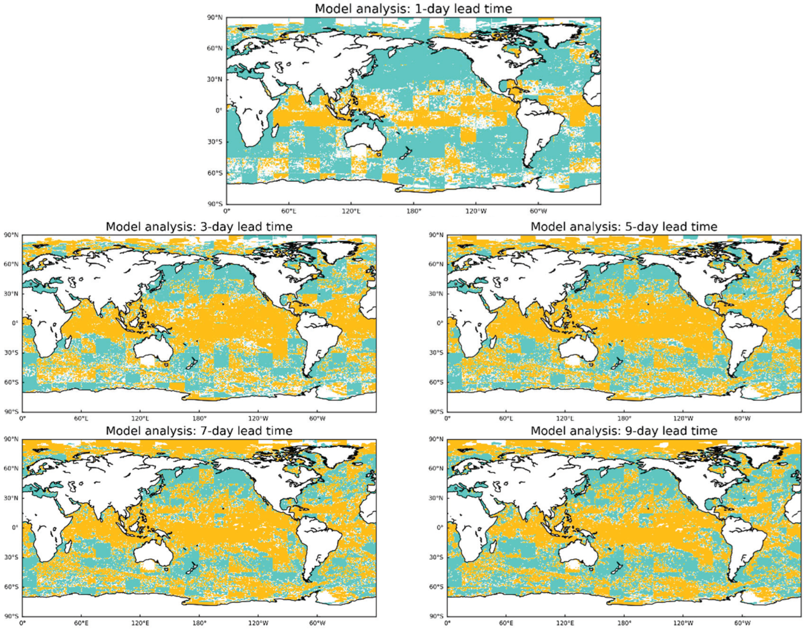
Figure 12 shows the degree of RMSE differences between MR-EDLSTM and MR-EDConvLSTM for global SST prediction, and the locations where MR-EDConvLSTM predicts better than MR-EDLSTM are shown in orange, and the opposite is shown in green. In Section 3.2, we know that MR-EDLSTM is better in predicting SST from day 1 to day 3. However, from Figure 12, we find that the MR-EDLSTM model does not perform as well as the MR-EDConvLSTM model in predicting day 1, day 3, day 5, day 7, and day 9 near the latitude 0° sea area.

Therefore, we conclude the following:

(1) The MR-EDLSTM model is more suitable for predicting SST in coastal areas in contact with land, such as the eastern part of Asia, the eastern and northwestern parts of the Americas, and other coastal areas.

(2) The MR-EDConvLSTM model is more suitable for predicting SST in seas near the equator, such as the Pacific, Indian, and Atlantic Oceans near the equator.

5. Conclusions

This paper focuses on a global SST prediction method based on deep learning. By using the dynamic region partitioning method, the global sea area is divided into several equal-sized blocks, and the global SST prediction is realized via the multi-region and multi-model framework. Using the idea of migration learning, the model is only initialized once and trained on the basis of the original weights when training other regions, which accelerates the training speed of the model and reduces the running memory consumption. The proposed MR-EDLSTM model is better at prediction of global SST, with RMSE and PACC reaching 0.2712 °C and 98.81% on the first day. In terms of SST seasonal prediction, the proposed model has a smaller RMSE between January and April and November and December, however, the prediction error is relatively larger between May and October. Compared with the LICOM marine environmental forecasting system (LFS) based on the ocean model, the RMSE of the deep learning model is smaller from day 1 to day 7, which indicates that the model has higher prediction ability and verifies the advantage of the deep learning method in predicting global SST.

In our future work, we will continue to improve the model, optimize the global prediction framework, improve the prediction speed, and extend it to the field of spatio-temporal series prediction of other marine environmental elements.

References

1. Acero, W.G.; Li, L.; Gao, Z.; Moan, T. Methodology for assessment of the operational limits and operability of marine operations. Ocean Eng. 2016, 125, 308–327. [Google Scholar] [CrossRef]
2. Formela, K.; Weintrit, A.; Neumann, T. Overview of definitions of maritime safety, safety at sea, navigational safety and safety in general. TransNav Int. J. Mar. Navig. Saf. Sea Transp. 2019, 13, 285–290. [Google Scholar] [CrossRef]
3. Kudela, R.M.; Bickel, A.; Carter, M.L.; Howard, M.; Rosenfeld, L. The monitoring of harmful algal blooms through ocean observing: The development of the California Harmful Algal Bloom Monitoring and Alert Program. In Coastal Ocean Observing Systems; Academic Press: Pittsburgh, PA, USA, 2015; pp. 58–75. [Google Scholar] [CrossRef]
4. Johnson, G.C.; Lyman, J.M. Warming trends increasingly dominate global ocean. Nat. Clim. Chang. 2020, 10, 757–761. [Google Scholar] [CrossRef]
5. Zhang, Y.; Wang, R.; Yang, M.; Zhu, M.; Ye, C. Using full-traversal addition-subtraction frequency (ASF) method to predict possible el nino events in 2019, 2020 and so forth. In Proceedings of the 2018 Chinese Control And Decision Conference, Shenyang, China, 9–11 June 2018; pp. 2652–2657. [Google Scholar] [CrossRef]
6. Li, Z.; He, J.; Ni, T.; Huo, J. Numerical computation based few-shot learning for intelligent sea surface temperature prediction. Multimed. Syst. 2022, 1–13. [Google Scholar] [CrossRef]
7. Kug, J.S.; Kang, I.S.; Lee, J.Y.; Jhun, J.G. A statistical approach to Indian Ocean sea surface temperature prediction using a dynamical ENSO prediction. Geophys. Res. Lett. 2004, 31, L09212. [Google Scholar] [CrossRef]
8. Zhao, Y.; Yang, D.; He, Z.; Liu, C.; Hao, R.; He, J. Statistical Methods in Ocean Prediction. In Proceedings of the Global Oceans 2020: Singapore–US Gulf Coast, Biloxi, MS, USA, 5–30 October 2020; pp. 1–7. [Google Scholar] [CrossRef]
9. Hernandez, F.; Smith, G.; Baetens, K.; Cossarini, G.; Garciahermosa, I.; Drevillon, M.; Maksymczuk, J.; Melet, A.; Regnier, C.; Schuckmann, K. Measuring Performances, Skill and Accuracy in Operational Oceanography: New Challenges and Approaches. In New Frontiers in Operational Oceanography; Amazon Press: Washington, DC, USA, 2018; pp. 759–796. [Google Scholar] [CrossRef]
10. Fang, W.; Sha, Y.; Sheng, V.S. Survey on the Application of Artificial Intelligence in ENSO Forecasting. Mathematics 2022, 10, 3793. [Google Scholar] [CrossRef]
11. Wen, J.; Yang, J.; Jiang, B.; Song, H.; Wang, H. Big data driven marine environment information forecasting: A time series prediction network. IEEE. Trans. Fuzzy Syst. 2021, 29, 4–18. [Google Scholar] [CrossRef]
12. Pauthenet, E.; Bachelot, L.; Balem, K.; Maze, G.; Treguier, A.M.; Roquet, F.; Fablet, R.; Tandeo, P. Four-dimensional temperature, salinity and mixed layer depth in the Gulf Stream, reconstructed from remote sensing and in situ observations with neural networks. Ocean Sci. 2022, 18, 1221–1244. [Google Scholar] [CrossRef]
13. de Mattos Neto, P.S.; Cavalcanti, G.D.; de O Santos Júnior, D.S.; Silva, E.G. Hybrid systems using residual modeling for sea surface temperature forecasting. Sci. Rep. 2022, 12, 487. [Google Scholar] [CrossRef]
14. Menaka, D.; Gauni, S.; Indiran, G.; Venkatesan, R.; Arul Muthiah, M. Development of heuristic neural network algorithm for the prognosis of underwater ocean parameters. Mar. Geophys. Res. 2022, 43, 40–58. [Google Scholar] [CrossRef]
15. Zhu, Y.; Bo, Y.; Zhang, J.; Wang, Y. Fusion of multisensor SSTs based on the spatiotemporal hierarchical Bayesian model. J. Atmos. Ocean. Technol. 2018, 31, 91–109. [Google Scholar] [CrossRef]
16. Lins, I.D.; Araujo, M.; Moura, M.; Silva, M.; Droguett, E.L. Prediction of sea surface temperature in the tropical Atlantic by support vector machines. Comput. Stat. Data Anal. 2013, 61, 187–198. [Google Scholar] [CrossRef]
17. Lins, I.D.; Veleda, D.; Araujo, M.; Silva, M.; Droguett, E.L. Prediction of surface meteorological variables in the southwestern tropical Atlantic by support vector machines. In Safety, Reliability and Risk Analysis; Taylor & Francis Group Press: London, UK, 2013; pp. 3287–3293. [Google Scholar] [CrossRef]
18. Pisoni, E.; Pastor, F.; Volta, M. Artificial Neural Networks to reconstruct incomplete satellite data: Application to the Mediterranean Sea Surface Temperature. Nonlin. Processes Geophys. 2008, 15, 61–70. [Google Scholar] [CrossRef]
19. Fan, F.; Xiong, J.; Li, M.; Wang, G. On interpretability of artificial neural networks: A survey. IEEE Trans. Radiat. Plasma Med. Sci. 2021, 5, 741–760. [Google Scholar] [CrossRef]
20. Cierniak, R. A New Approach to Image Reconstruction from Projections Using a Recurrent Neural Network. Int. J. Appl. Math. Comput. Sci. 2008, 18, 147–157. [Google Scholar] [CrossRef]
21. Xie, Z.; Jin, L.; Luo, X.; Sun, Z.; Liu, M. RNN for repetitive motion generation of redundant robot manipulators: An orthogonal projection-based scheme. IEEE Trans. Neural Netw. Learn. Syst. 2022, 33, 615–628. [Google Scholar] [CrossRef] [PubMed]
22. Hinton, G.E.; Salakhutdinov, R.R. Reducing the dimensionality of data with neural networks. Science 2006, 313, 504–507. [Google Scholar] [CrossRef] [Green Version]
23. Tran, D.; Bourdev, L.; Fergus, R.; Torresani, L.; Paluri, M. Learning spatiotemporal features with 3d convolutional networks. In Proceedings of the IEEE International Conference on Computer Vision, Santiago, Chile, 13–16 December 2015; pp. 4489–4497. [Google Scholar] [CrossRef] [Green Version]
24. Wang, G.G.; Cheng, H.; Zhang, Y.; Yu, H. ENSO analysis and prediction using deep learning: A review. Neurocomputing 2023, 520, 216–229. [Google Scholar] [CrossRef]
25. Goroshin, R.; Mathieu, M.; Lecun, Y. Learning to linearize under uncertainty. In Proceedings of the 28th International Conference on Neural Information Processing Systems, Montreal, QC, Canada, 7–12 December 2015; pp. 1234–1242. [Google Scholar] [CrossRef]
26. Mathieu, M.; Couprie, C.; Lecun, Y. Deep multi-scale video prediction beyond mean square error. In International Conference on Learning Representations; ICLR Press: San Juan, Puerto Rico, 2016; pp. 1–14. [Google Scholar] [CrossRef]
27. Hochreiter, S.; Schmidhuber, J. Long short-term memory. Neural. Comput. 1997, 9, 1735–1780. [Google Scholar] [CrossRef] [PubMed]
28. Graves, A. Long short-term memory. Supervised Seq. Label. Recurr. Neural Netw. 2012, 385, 37–45. [Google Scholar] [CrossRef]
29. Srivastava, N.; Mansimov, E.; Salakhutdinov, R. Unsupervised learning of video representations using lstms. In Proceedings of the 32nd International Conference on Machine Learning; JMLR Press: Lille, France, 2015; pp. 843–852. [Google Scholar] [CrossRef]
30. Oh, J.; Guo, X.; Lee, H.; Lewis, R.L.; Singh, S. Action-conditional video prediction using deep networks in atari games. In Proceedings of the 28th International Conference on Neural Information Processing Systems, Montreal, QC, Canada, 7–12 December 2015; pp. 2863–2871. [Google Scholar] [CrossRef]
31. Wu, A.; Hsieh, W.W.; Tang, B. Neural network forecasts of the tropical Pacific sea surface temperatures. Neural. Netw. 2006, 19, 145–154. [Google Scholar] [CrossRef] [Green Version]
32. Wei, L.; Guan, L.; Qu, L. Prediction of sea surface temperature in the South China Sea by artificial neural networks. IEEE Geosci. Remote Sens. Lett. 2020, 17, 558–562. [Google Scholar] [CrossRef]
33. Qin, Z.; Hui, W.; Dong, J.; Zhong, G.; Xin, S. Prediction of Sea Surface Temperature using Long Short-Term Memory. IEEE Geosci. Remote Sens. Lett. 2017, 14, 1745–1749. [Google Scholar] [CrossRef] [Green Version]
34. Yang, Y.; Dong, J.; Sun, X.; Lima, E.; Mu, Q.; Wang, X. A CFCC-LSTM model for sea surface temperature prediction. IEEE Geosci. Remote Sens. Lett. 2018, 15, 207–211. [Google Scholar] [CrossRef]
35. Lin, Y.; Zhong, G. A Multi-Channel LSTM Model for Sea Surface Temperature Prediction. J. Phys. Conf. Ser. 2021, 1880, 012029–012034. [Google Scholar] [CrossRef]
36. Hou, S.; Li, W.; Liu, T.; Zhou, S.; Guan, J.; Qin, R.; Wang, Z. MIMO: A Unified Spatio-Temporal Model for Multi-Scale Sea Surface Temperature Prediction. Remote Sens. 2022, 14, 2371. [Google Scholar] [CrossRef]
37. Shi, X.; Chen, Z.; Wang, H.; Yeung, D.Y.; Wong, W.K.; Woo, W.C. Convolutional LSTM network: A machine learning approach for precipitation nowcasting. In Proceedings of the 28th International Conference on Neural Information Processing Systems, Montreal, QC, Canada, 7–12 December 2015; pp. 802–810. [Google Scholar] [CrossRef]
38. Zhang, K.; Geng, X.; Yan, X.H. Prediction of 3-D ocean temperature by multilayer convolutional LSTM. IEEE Geosci. Remote Sens. Lett. 2020, 17, 1303–1307. [Google Scholar] [CrossRef]
39. Li, C.; Feng, Y.; Sun, T.; Zhang, X. Long Term Indian Ocean Dipole (IOD) Index Prediction Used Deep Learning by convLSTM. Remote Sens. 2022, 14, 523. [Google Scholar] [CrossRef]
40. Xu, L.; Li, Q.; Yu, J.; Wang, L.; Shi, S. Spatio-temporal predictions of SST time series in China’s offshore waters using a regional convolution long short-term memory (RC-LSTM) network. Int. J. Remote Sens. 2020, 41, 3368–3389. [Google Scholar] [CrossRef]
41. Gou, Y.; Zhang, T.; Liu, J.; Wei, L.; Cui, J.H. DeepOcean: A general deep learning framework for spatio-temporal ocean sensing data prediction. IEEE Access 2020, 8, 79192–79202. [Google Scholar] [CrossRef]
42. Wei, L.; Guan, L.; Qu, L.; Guo, A.D. Prediction of sea surface temperature in the China seas based on long short-term memory neural networks. Remote Sens. 2020, 12, 2697. [Google Scholar] [CrossRef]
43. Jia, X.; Ji, Q.; Han, L.; Liu, Y.; Han, G.; Lin, X. Prediction of Sea Surface Temperature in the East China Sea Based on LSTM Neural Network. Remote Sens. 2022, 14, 3300. [Google Scholar] [CrossRef]
44. Chen, K.; Kuang, C.; Wang, L.; Chen, K.; Han, X.; Fan, J. Storm surge prediction based on long short-term memory neural network in the East China Sea. Appl. Sci. 2022, 12, 181. [Google Scholar] [CrossRef]
45. Sarkar, P.P.; Janardhan, P.; Roy, P. A novel deep neural network model approach to predict Indian Ocean dipole and Equatorial Indian Ocean oscillation indices. Dyn. Atmos. Oceans 2021, 96, 101266. [Google Scholar] [CrossRef]
46. Ali, M.M.; Swain, D.; Kashyap, T.; Mccreary, J.P.; Nagamani, P.V. Relationship between cyclone intensities and sea surface temperature in the tropical Indian Ocean. IEEE Geosci. Remote Sens. Lett. 2013, 10, 841–844. [Google Scholar] [CrossRef]
47. Sai, P.M.; Vasavi, S.; Vighneshwar, S.P. Prediction of temperature anomaly in Indian Ocean based on autoregressive long short-term memory neural network. Neural. Comput. Appl. 2022, 34, 7537–7545. [Google Scholar] [CrossRef]
48. Avsar, N.B.; Jin, S.; Kutoglu, S.H. Interannual variations of sea surface temperature in the Black Sea. In Proceedings of the IEEE International Geoscience and Remote Sensing Symposium, Valencia, Spain, 22–27 July 2018; pp. 5617–5620. [Google Scholar] [CrossRef]
49. Reynolds, R.W.; Smith, T.M.; Liu, C.; Chelton, D.B.; Casey, K.S.; Schlax, M.G. Daily high-resolution-blended analyses for sea surface temperature. J. Clim. 2007, 20, 5473–5496. [Google Scholar] [CrossRef]
50. Kingma, D.; Ba, J. Adam: A Method for Stochastic Optimization. In Proceedings of the 3rd International Conference on Learning Representations, San Diego, CA, USA, 7–9 May 2015; pp. 1–15. [Google Scholar] [CrossRef]
51. Li, Y.; Liu, H.; Ding, M.; Lin, P.; Yu, Z.; Yu, Y.; Meng, Y.; Li, Y.; Jian, X.; Jiang, J.; et al. Eddy-resolving Simulation of CAS-LICOM3 for Phase 2 of the Ocean Model Intercomparison Project. Adv. Atmos. Sci. 2020, 37, 1067–1080. [Google Scholar] [CrossRef]
52. Lin, P.; Yu, Z.; Liu, H.; Yu, Y.; Ma, J. LICOM Model Datasets for the CMIP6 Ocean Model Intercomparison Project. Adv. Atmos. Sci. 2020, 37, 239–249. [Google Scholar] [CrossRef] [Green Version]
53. Liu, H.; Lin, P.; Zheng, W.; Luan, Y.; Ma, J.; Ding, M.; Mo, H.; Wan, L.; Ling, T. A global eddy-resolving ocean forecast system in China-LICOM Forecast System (LFS). J. Oper. Oceanog. 2023, 16, 15–27. [Google Scholar] [CrossRef]
Figure 1. Workflow of the global SST prediction framework.
Jmse 11 01352 g001
Figure 2. Schematic representation of sample data set generation during data pre-processing.
Jmse 11 01352 g002
Figure 3. Structure of the LSTM cell [27].
Jmse 11 01352 g003
Figure 4. Global SST prediction results for day 1, day 3, day 5, day 7, and day 9.
Jmse 11 01352 g004
Figure 5. Global SST prediction errors for day 1, day 3, day 5, day 7, and day 9.
Jmse 11 01352 g005
Figure 6. Statistics of Global SST prediction errors for day 1.
Jmse 11 01352 g006
Figure 7. Results of Area_RMSE predicted by the model in 365 experiments for day 1, day 3, day 5, day 7, and day 9.
Jmse 11 01352 g007
Figure 8. Results of Area_ACC predicted by the model in 365 experiments for day 1, day 3, day 5, day 7, and day 9.
Jmse 11 01352 g008
Figure 9. Comparison of RMSE between deep learning and LFS methods.
Jmse 11 01352 g009
Figure 10. RMSE for global SST predictions for each location on day 1, day 3, day 5, day 7, and day 9.
Jmse 11 01352 g010
Figure 11. Statistics of RMSE for day 1, day 3, and day 5. The different RMSE ranges as a percentage of the total are indicated by different colors.
Jmse 11 01352 g011
Figure 12. Degree of difference in RMSE for global SST predictions for each location between MR-EDLSTM and MR-EDConvLSTM. The locations where MR-EDConvLSTM predicts better than MR-EDLSTM are shown in orange, and the opposite is shown in green.
Jmse 11 01352 g012